Abstract
The simulation of electronic control function failure has been utilized broadly as an evaluation method when determining the Automotive Safety Integrity Level (ASIL). The driver model is quite critical in the ASIL evaluation simulation. A new driver model that can consider drivers of different driving skills is proposed in this paper. It can simulate the overall performance of different drivers driving vehicles by adjusting parameters, with which the impact of a certain electronic control function failure and the ASIL are evaluated. This paper has taken the function failure of regenerative braking as the simulation object in the double-lane-change driving scenario to simulate typical driving conditions with the designed driver model, and then has obtained the ASIL of regenerative braking function, which is applied to a BAIC new energy vehicle development project.
1. Introduction
More and more electronic control functions have been integrated into vehicles with the improvement of vehicle electrification in recent years [1]. In order to ensure vehicle safety, functional safety design should be taken into consideration for the electronic control system [2,3,4]. A functional safety rating is the key to functional safety design. When assessing the functional safety level, it is necessary to simulate the potential accidents caused by the electronic control function failure regarding the controllability, severity, and fault tolerance time [5,6]. To simulate electronic control function failure and its effect, the most widely used method is by computer simulation, which uses a virtual model of the “driver-vehicle-environment” system [7] to obtain the final data under different dangerous driving conditions. The driver, vehicle, and environment sub-models should be as close as possible to the real situation in the abovementioned virtual model. At present, the design technology of vehicle and environment sub-models is relatively mature, while the research of driver sub-model applied to Automotive Safety Integrity Level (ASIL) simulation is still in the early phase. One of the design difficulties is how to design a reliable model that can simulate drivers with different driving skills to improve the simulation results.
When driving the vehicle, the driver firstly decides the target route which is to be tracked by turning the steering wheel based on the experience of the vehicle’s steering characteristics, while maintaining vehicle stability. Existing research shows that when the steering wheel is turned by different drivers there are two critical parameters—vehicle lateral displacement and yaw angle status [8,9,10]. For drivers with poor driving experience, the vehicle is equivalent to a particle, so that more consideration is given to whether the vehicle displacement is consistent with driver expectations. Drivers with significant driving experience pay more attention to the smooth adjustment of the vehicle’s yaw status to ensure that the vehicle’s real driving route meets requirements with high stability control. The steering wheel angle is determined by the difference between vehicle lateral displacement and the target route, which needs to be accurately calculated and has a direct impact on vehicle tracking accuracy. The driver model proposed in the existing literature uses vehicle longitudinal displacement and the relation between longitudinal displacement and lateral displacement during the preview time to identify the position of the target point when calculating the lateral displacement difference [11]. The target point determined at the last moment cannot be reached due to the real-time change of steering wheel angle when turning the vehicle. Besides, the existing algorithms lack consideration regarding the influence of steering wheel angle on the vehicle driving stability when determining the steering wheel angle.
Based on accurate prediction of the difference of vehicle lateral displacement, this article proposes a dual-objective optimized control strategy that considers vehicle tracking ability and driving stability and contains settable parameters according to the driver’s driving reaction, which differs due to individual driving skill level when the electronic control function fails. In the end, the effect of electronic control function failure and its ASIL can be concluded.
2. Driver Model Based on Multi-Objective Optimization
Compared with the multi-point preview or interval preview method, there is no need to accumulate or integrate differences at multiple preview points within the preview time using the single-point preview method, which suggests a simple calculation. In addition, with a single-point preview method, only one point on the target route is used, which results in a better tracking ability under stable driving. Due to the lack of optimization on vehicle driving stability during the entire preview period, the single-point preview model proposed in the existing literature can hardly keep the vehicle in an optimized lateral adhesion condition, especially when the curvature is large and the adhesion is poor on the target route. In order to establish a simulation model with a small amount of calculation, accurate tracking ability, and prevention of vehicle instability due to incorrect steering wheel angle input, this article proposes an algorithm using the single-point preview method with consideration of vehicle lateral adhesion condition for determination of the steering wheel angle.
In the proposed driver model, the steering wheel angle is optimized with consideration of both the vehicle lateral displacement difference and the lateral deviation of vehicle front and rear axles. It is divided into the following steps in detail: firstly, the target route in the preview interval is identified according to the planned driving route. Secondly, the steering angle is determined to minimize the difference between vehicle position and target route in both lateral and longitudinal direction, and to optimize vehicle steering characteristics.
2.1. Calculation of Steering Wheel Angle
2.1.1. Determination of Target Route
In the vehicle coordinate system, the function of fitting the horizontal coordinate of the target route to the vertical coordinate is the following:
where are the - and -component of the vehicle route, respectively. When turning the vehicle, , and the target route is a non-linear function. In this paper, considering that the driver only drives the vehicle along a parabolic trajectory during the short preview time, the target route is fitted to a quadratic function as follows:
2.1.2. Determination of Lateral Displacement Difference
To acquire the displacement in the current coordinate system after preview interval , a simplified 2-DOF vehicle model is introduced in Figure 1 [12]. Symbolic variables stand for the velocity at the front and rear wheels, respectively, while is the wheelbase; are the lateral forces acted on the front and rear wheels, are the slip angles, and are the longitudinal and lateral velocity of the vehicle, respectively, are the lateral acceleration and yaw rate.
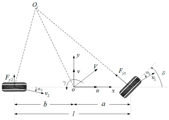
Figure 1.
A 2-DOF vehicle model.
The displacement can be obtained according to the above model,
As , , this can be solved,
Therefore, the abscissa of the preview point . Further, we have and . Assume and represent the cornering stiffnesses of front and rear axles while is the moment of inertia about axis, is the slip angle of the mass center. Then, the following equation is achieved:
Thus,
2.1.3. Constraints of Vehicle Steering Characteristics
When determining the wheel angle, the balance between slip angles of the vehicle’s front and rear axles is considered in this paper. According to the kinematics relation in the 2-DOF model [13], the following equations can be obtained:
When the two slip angles satisfy , the vehicle is in neutral steering. Therefore, the following equation is introduced to characterize the influence of the steering wheel angle on the vehicle steering characteristics,
which could be further written as:
Equation (8) uses the difference between the front and rear axle tire sideslip angles to characterize the steering characteristics of the vehicle. Equation (7) describes that this difference is a linear function of the steering angle.
2.1.4. Optimized Control of Steering Wheel Angle
It is assumed that when the driver is deciding the steering wheel angle, the lateral displacement difference between vehicle and preview point and the slip angle difference are both minimized. This could be abstracted into solving the following optimized problem [14]:
where the objective function could be written as:
and , represent the weight coefficient of lateral displacement difference and slip angle difference respectively, when determining steering wheel angle.
2.2. Solution to the Problem
This paper establishes a linear transferring relationship from steering wheel angle to vehicle lateral acceleration and yaw acceleration based on a simplified vehicle model. However, the target route in the vehicle coordinate system is a non-linear function, which leads to a nonlinear relationship between and wheel angle in the optimized objective function; the optimization objective is a high-order function of the wheel angle .
A simplified solution that takes both calculation cost and accuracy of the result into account is then adopted. It is assumed that the velocity is constant during the preview interval, based on which the exact position of the preview point is obtained. Then, the objective function is simplified from a high-order function to a quadratic one that could be resolved for an initial optimized point .
Assuming the vehicle is turning steadily with a constant velocity in preview interval , and the position of the vehicle is calculated after the preview period, when the wheel angle is modified from to , the lateral displacement difference is the following:
where describes the variation in lateral acceleration generated after the steering wheel angle is altered, relationships and are then satisfied. The multi-objective optimization is transformed into quadratic convex optimization that could be expressed as,
To simplify it for a solution, the optimization is the following:
where in which and , and in which,
and,
The solution to the optimization issue [15] could be obtained,
2.3. Steering Wheel Angle Relevant to the Driver’s Response Lag
After the optimum steering wheel angle is defined, the driver controls the steering wheel to follow the target value. Taking into account the response lag of the human nervous system and inertial response lag, the lag processing step is added [16,17]. Finally, the relation of steering wheel angle and its theoretical optimum value is the following:
In the lag processing step, represents the inertial response lag of the driver when controlling the steering wheel, and characterizes the response lag of the human nervous system. In the low-frequency range,
where is the lag time of the nervous system.
3. Model Simulation and Verification
3.1. Model Overview
The model for simulation in this article consists of models of a driver, electronic drive system, brake system, wheel, and body motion. It also differs in terms of roads status with variable grades and adhesion coefficients. The vehicle model has eight degrees of freedom [18]: lateral and longitudinal velocity, yaw velocity, revolving speed of four wheels and the wheel angle. The system layout is illustrated in Figure 2.
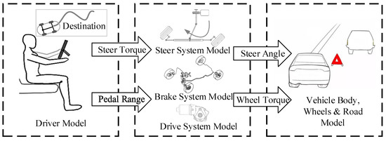
Figure 2.
Driver–vehicle–environment simulation model.
The road with a variable adhesion coefficient could be used to simulate the scenario on a rural road that is partly covered with either snow or ice. In this article, according to the wheel’s displacement, the contact torque between the tire and the road surface in the model reflects the impact on adhesion by a partially icy road [19], as Figure 3 demonstrates.
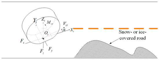
Figure 3.
The road model with variable adhesion coefficient.
3.2. Simulation Model Calibration and Verification
To assure the model accuracy, real vehicle tests are conducted on an EV160 from BAIC-EV. Model calibration and verification are then performed according to the data collected. The main parameters of the test vehicle can be found in Table 1.

Table 1.
Test vehicle parameters.
In order to complete the calibration and verification, two testing conditions are conducted for data collection. One is an acceleration and sliding experiment in a straight direction to validate the response characteristics of vehicle velocity with the input from the acceleration pedal. The other is the double-lane-change experiment that could verify the response characteristics of the vehicle’s steering status with the input from the steering wheel.
In the straight driving test, the driver releases the brake pedal after the vehicle starts to run and then quickly steps on the acceleration pedal to speed up the vehicle to 100 km/h. The pedal is then released while the driver only gets control of the steering wheel to maintain straight direction until the velocity reduces to around 6 km/h when the experiment ends. Throughout the experiment, the output driving torque, the regenerative braking torque, and revolving speed are collected from the electric motor. The input, being transferred into the driver–vehicle–environment model, includes acceleration pedal position and driving torque. The results are shown in Figure 4, Figure 5, Figure 6 and Figure 7.
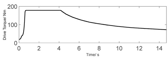
Figure 4.
Drive torque under straight driving.
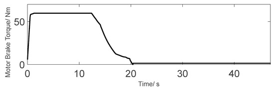
Figure 5.
Regenerative braking torque under straight driving.
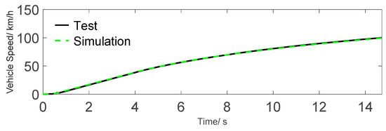
Figure 6.
Speed comparison during acceleration: simulation and real test.
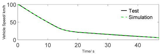
Figure 7.
Speed comparison during sliding braking.
In the double-lane-change experiment, a typical arrangement of the lane and roadblocks [20] is illustrated in Figure 8 where , , and stands for the width of the vehicle. The results are shown in Figure 9 and Figure 10.
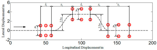
Figure 8.
A typical arrangement of the test. See the text for detail.
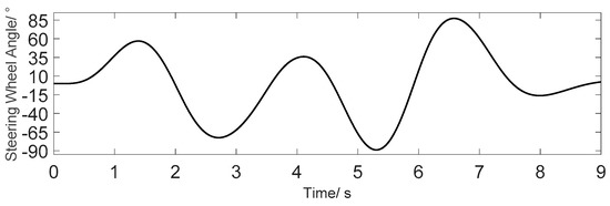
Figure 9.
The driver’s steering wheel angle input (versus time) under double-lane-change test.
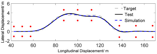
Figure 10.
Vehicle path comparison under double-lane-change.
4. Driver Model’s Application in Functional Safety Simulation
4.1. Driver Model Calibration
Thirty drivers with distinct genders and driving experiences were invited to conduct a double-lane-change experiment on EV160. During the test, the driver was required to keep the accelerator pedal and the brake pedal uncontrolled to track the target trajectory by turning the steering wheel, and the state parameters of each driver were recorded during the driving of the vehicle including four-wheel speed, vehicle longitudinal acceleration, lateral vehicle speed, yaw rate, GPS vehicle speed, steering wheel angle, vehicle longitudinal displacement, lateral displacement. According to Equation (17) and collected data, the least square method is used to obtain the characteristic parameters of each driver: where . In total, 30 sets of parameters can be obtained and each set of parameters is substituted into the driver model to characterize the driving performance in the actual double-lane change conditions. Figure 11 shows the driving data of 30 drivers and the driving trajectory of one “virtual driver”.
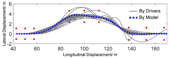
Figure 11.
Vehicle path of 30+1 different drivers under double-lane-change test.
4.2. Functional Safety Simulation with the New Driver Model
During the functional safety design for the regenerative braking control system [21,22,23], simulation is necessary to perform to acquire the severity, controllability, and fault tolerance time under the failure mode of “unexpected peak regenerative braking torque”.
4.2.1. Scenario Setting
This paper chooses the scenario with higher exposure rate to simulate the failure response, which is changing lanes with low speed on the slippery urban road under the condition of clear day. According to the external characteristics of the PMSM motor, in this low-speed scenario the regenerative braking torque can reach a peak, which is also a scenario when the risk of vehicle collision is higher than high-speed driving. As vehicle A runs on a wet urban road with an initial velocity of 30 km/h, the driver starts the double-lane change to avoid vehicle B [24] as well as vehicle C in the opposite lane. At this time, the maximum regenerative braking torque appears, causing the front axle of the vehicle to lock, and the steering is out of control, which may lead to a crash. The scenario is shown in Figure 12.
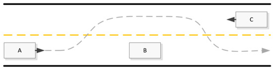
Figure 12.
A typical double-lane-change scenario for functional safety simulation.
4.2.2. Simulation Result
The results demonstrated in Figure 13 and Figure 14 show that when the peak regenerative braking torque was applied to the front axle, the driver lost vehicle control and the controllability was C3, which is a level in ISO26262 described as “uncontrollable condition”. Figure 15 gives the reason of reverse yaw shown in Figure 13. At this time, due to the lateral instability of the vehicle, the lane change was not completed in time which led to collision with vehicle B in the current lane. The collision speed was 24.9 km/h, so the severity is S2 according to ISO26262. Together with the wet road exposure rate E3, the functional safety level of the regenerative braking control system is ASIL B according to the calculation method of ASIL in ISO26262. Based on this, the safety goal is to “avoid peak regenerative braking torque during driving, which causes wheels locking and sideslip”. The corresponding safety status is “the regenerative braking torque output by the drive motor is zero”.
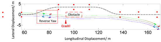
Figure 13.
Vehicle path in a failure scenario.
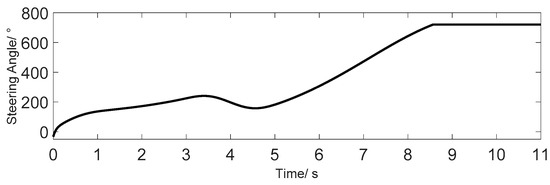
Figure 14.
Steering wheel angle input (from the driver).
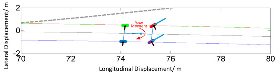
Figure 15.
Reverse yaw force analysis.
As shown in Figure 16, Figure 17 and Figure 18, it could be obtained from the result that when the maximum application time of unexpected peak torque is 300 ms, the driver is capable of controlling the vehicle to complete the double-lane change. Therefore, the fault tolerance time interval is determined as 300 ms.
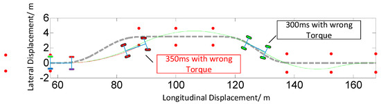
Figure 16.
FTT calculation by fault injection simulation.
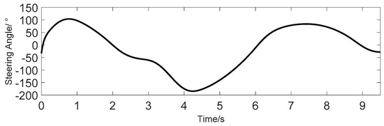
Figure 17.
Steering wheel angle (versus time) by the driver.
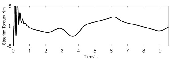
Figure 18.
Steering torque input (versus time) by the driver.
5. Conclusions
This paper proposes a new design of driver model based on multi-objective optimization, and functional safety simulation is carried out with it. Conclusions can be drawn as follows:
- (1)
- Steering wheel angle in preview interval is calculated based on deviation of sideslip angle between front and rear axle and minimizing lateral displacement difference. After steering wheel angle is obtained, drivers with different driving skills are simulated with definition of weight parameters in objective function of the multi-objective optimization.
- (2)
- A “driver-vehicle-environment” model is established. Simulation of a failed electronic control system is performed under the operation of different “drivers”, which helps eliminate the risk of accidents and is thus suitable for ASIL of an electronic control system.
- (3)
- After the simulation analysis, the functional safety goal is clearly defined for EV160 regenerative braking system under the condition of regenerative braking torque being out of control. The functional safety goal is to “avoid peak regenerative braking torque during driving, which causes wheels locking and sideslip. With ASIL B the fault tolerance time is 300 ms”.
Author Contributions
Formal analysis, X.Z.; Investigation, Z.Z.; Methodology, Y.Z.; Project administration, Z.X.; Visualization, H.W. All authors have read and agreed to the published version of the manuscript.
Funding
This work was supported in part by the National Natural Science Foundation of China under Grant 51775039, Grant 51861135301, and Grant 51805030; and in part by the Special Program for Science and Technology Funding for Innovative Talents under Grant 3052019009.
Acknowledgments
The authors would like to thank the reviewers for their corrections and helpful suggestions.
Conflicts of Interest
The authors declare no conflict of interest.
References
- Tang, M. Application Status and Development Trend of Electronic Technology in Automobile. DEStech Trans. Eng. Technol. Res. 2016, 180–184. [Google Scholar] [CrossRef]
- Qin, R.; Xiaodong, W.; Min, X. Functional safety concept design for steer-by-wire system of road vehicle based on the ISO. J. Automot. Saf. Energy 2018, 9, 250–257. [Google Scholar]
- Cheon, J.S.; Kim, J.; Jeon, J.; Lee, S.M. Brake by Wire Functional Safety Concept Design for ISO/DIS 26262. In SAE Technical Paper; SAE International: Warrendale, PA, USA, 2011. [Google Scholar]
- Burton, S.; Likkei, J.; Vembar, P.; Wolf, M. Automotive Functional Safety = Safety + Security. In Proceedings of the First International Conference on Security of Internet of Things, Zurich, Switzerland, 26–28 March 2008; Association for Computing Machinery: New York, NY, USA, 2012; pp. 150–159. [Google Scholar]
- International Standard ISO/FDIS Road Vehicles-Functional Safety (ISO26262); ISA: Geneva, Switzerland, 2018.
- Frese, T.; Leonhardt, T.; Hatebur, D.; Côté, I.; Aryus, H.-J.; Heisel, M. Fault Tolerance Time Interval. In Neue Dimensionen der Mobilität: Technische und betriebswirtschaftliche Aspekte (in German); Proff, H., Ed.; Springer Fachmedien: Wiesbaden, Germany, 2020; pp. 559–567. ISBN 978-3-658-29746-6. [Google Scholar]
- Butler, K.L.; Ehsani, M.; Kamath, P. Kamath A Matlab-based modeling and simulation package for electric and hybrid electric vehicle design. IEEE Trans. Veh. Technol. 1999, 48, 1770–1778. [Google Scholar] [CrossRef]
- Hess, R.A.; Modjtahedzadeh, A. A control theoretic model of driver steering behavior. IEEE Control Syst. Mag. 1990, 10, 3–8. [Google Scholar] [CrossRef]
- Ding, H.; Guo, K.; Li, F.; Zhang, J. Arbitrary path and speed following driver model based on vehicle acceleration feedback. Chin. J. Mech. Eng. 2010, 46, 116–120. [Google Scholar] [CrossRef]
- Jalali, K.; Lambert, S.; McPhee, J. Development of a Path-following and a Speed Control Driver Model for an Electric Vehicle. UWSpace 2012. [Google Scholar] [CrossRef]
- Nenggen, D.; Xiaofeng, R.; Hongbing, Z. Driver model for single track vehicle based on single point preview optimal curvature model. Chin. J. Mech. Eng. 2008, 44, 220–223. (In Chinese) [Google Scholar]
- Jazar, R.N. Vehicle Dynamics-Theory and Application, 3rd ed.; Springer: Berlin/Heidelberg, Germany, 2017; ISBN 978-3-319-53440-4. [Google Scholar]
- Mastinu, G.; Ploechl, M. Road and Off-Road Vehicle System Dynamics Handbook; CRC Press: Boca Raton, FL, USA, 2014; ISBN 978-0-8493-3322-4. [Google Scholar]
- Lin, C.; Xu, Z. Wheel Torque Distribution of Four-Wheel-Drive Electric Vehicles Based on Multi-Objective Optimization. Energies 2015, 8, 3815–3831. [Google Scholar] [CrossRef]
- Boggs, P.T.; Tolle, J.W. Tolle Sequential quadratic programming. Acta Numer. 1995, 4, 1–51. [Google Scholar] [CrossRef]
- McGehee, D.V.; Mazzae, E.N.; Baldwin, G.S. Scott Baldwin Driver reaction time in crash avoidance research: Validation of a driving simulator study on a test track. In Proceedings of the Human Factors and Ergonomics Society Annual Meeting, San Diego, CA, USA, 30 July–4 August 2000; Volume 44, pp. 3–320. [Google Scholar]
- Zhang, L.; Li, L.; Qi, B.; Song, J. High speed stability electromechanical coupling control for dual-motor distributed drive electric vehicle (in Chinese). Chin. J. Mech. Eng. 2015, 51, 29–40. [Google Scholar] [CrossRef]
- Bera, T.K.; Bhattacharya, K.; Samantaray, A.K. Evaluation of antilock braking system with an integrated model of full vehicle system dynamics. Simul. Model. Pract. Theory 2011, 19, 2131–2150. [Google Scholar] [CrossRef]
- Pacejka, H.B.; Bakker, E. The Magic Formula Tyre Model. Veh. Syst. Dyn. 1992, 21, 1–18. [Google Scholar] [CrossRef]
- ISO 3888-1:2018. Passenger Cars—Test Track for a Severe Lane-Change Manoeuvre—Part 1: Double Lane-Change 2018; ISO: Geneva, Switzerland, 2018.
- Zhang, Z. Design and Research of Braking Energy Recovery System for Pure Electric Vehicle; Beijing Institute of Technology: Beijing, China, 2016. [Google Scholar]
- Zhu, D.; Wang, X.; Li, Y.; Wang, Y. Research on Energy regenerative braking of electric vehicle based on functional safety analysis. In Proceedings of the 2017 2nd Asia-Pacific Conference on Intelligent Robot Systems (ACIRS), Wuhan, China, 16–19 June 2017; pp. 326–330. [Google Scholar]
- Koga, H.; Handa, K.; Kawai, N.; Saga, K.; Furukawa, N.; Maeda, A.; Oowada, T.; Yoshida, H. Regenerative Braking Control System for Electric Vehicle. U.S. Patent US 6,033,041, 7 March 2000. [Google Scholar]
- State Council in PRC. Regulations for the Implementation of the Road Traffic Safety Law of the People’s Republic of China; State Council in PRC: Shanghai, China, 2004. [Google Scholar]
Publisher’s Note: MDPI stays neutral with regard to jurisdictional claims in published maps and institutional affiliations. |
© 2020 by the authors. Licensee MDPI, Basel, Switzerland. This article is an open access article distributed under the terms and conditions of the Creative Commons Attribution (CC BY) license (http://creativecommons.org/licenses/by/4.0/).