Article

A Sustainable Distribution Design for Multi-Quality Multiple-Cold-Chain Products: An Integrated Inspection Strategies Approach

1
NUST Business School, National University of Science and Technology, Islamabad 44000, Pakistan
2
Industrial Engineering Department, College of Engineering, King Saud University, P.O. Box 800, Riyadh 11421, Saudi Arabia
3
Department of Management Systems and Logistics, Rzeszow University of Technology, 35-959 Rzeszow, Poland
4
College of Management, Research Institute of Business Analytics and Supply Chain Management, Shenzhen University, Shenzhen 518060, China
5
Department of Mechanical Engineering Technology, University of Technology, Nowshera 24100, Pakistan
6
Design, Manufacturing & Engineering Management, University of Strathclyde, Glasgow G1 1XJ, UK
7
Mechanical Engineering, Imperial College London, Exhibition Road, South Kensington, London SW7 2AZ, UK
*
Authors to whom correspondence should be addressed.
Energies 2020, 13(24), 6612; https://doi.org/10.3390/en13246612
Submission received: 19 November 2020 / Revised: 10 December 2020 / Accepted: 12 December 2020 / Published: 15 December 2020
(This article belongs to the Special Issue Energy Management Systems in Enterprises and Supply Chains)

Abstract

:
Cold-chain products are time-sensitive and perishable and pose the risk of failure if they are transported to a distant location. Thus, there is a need to analyze their quality during distribution so that the customers may receive optimal-quality products. To address this issue, this study integrates inspection strategies with the sustainable distribution system of multi-quality multiple-cold-chain products. A bi-objective model of cost and emission is proposed under the constraints of heterogeneous vehicle and time window. Furthermore, this study intends to address the following questions: which inspection strategy helps to ensure the potency of delivered products, and what is the impact of quality differentiation on the value of objective functions? A set of meta-heuristics is used for implementing the model using a rich panel of experiments. The results reveal that the quality conditions of different products impact the solutions of cost and emissions. Moreover, the conformity strategy is more viable, as it results in less cost and ensures that the quantity of delivered products meets the level of demand. Finally, the study provides implications for managers and practitioners to develop a sustainable distribution system to maintain the quality of cold-chain products.

1. Introduction

The cold chain is designed to store, transport, and deliver products from production facility to customer-preferred locations [1,2,3]. Such products are perishable as they have a limited shelf life. Thus, it becomes a challenge to design sustainable distribution in a way to minimize the spoilage issues and waste [4]. These products can be categorized into food and fruit items, medicines, vaccines, and many more similar products. Sustainable distribution design of such products differs from other supply chains in many aspects (e.g., refrigeration and emission of different gases). One of the research goals in the existing cold-chain literature is to minimize environmental concerns and to reduce its impact on global warming along with economic and responsiveness dimensions [5]. Research findings show that the cold-chain distribution system has become a major environmental concern and it contributed by 14% to the worldwide emission of greenhouse gases in 2010 [6].
There is always a trade-off in the distribution design of cold-chain products. On the one hand, economic value is to be generated by timely delivery of products in their potent state. On the other hand, environmental protection is to be considered, which can affect profit margins. Cold-chain products have become a priority for customers [7]. An increase in the demand of cold-chain products has been observed in the era of COVID-19. Due to social distancing, many customers have been reluctant to go out for shopping during the lockdown and have preferred to purchase products using online platforms. In some European countries, online businesses (such as Amazon) could ship only a limited type of products and the list comprised health-related products (medicines), food items, and technology-based products. The importance of the cold chain was well established in a report published by the USA commerce department (International Trade Administration) [8]. According to the report: (a) an annual loss worth one billion USD is observed in the food industry due to improper storage mechanism and poor handling; (b) more than 130 billion USD value of sales rely on the effectiveness of the cold chain to ensure the potency and quality of delivered products; and (c) the cold chain of perishable food products is approximately worth 250 billion USD annually. Considering such figures, the cold chain has a worldwide footprint, and thus its importance cannot be neglected both from research and practice viewpoints.
Research on the cold chain primarily focuses on vehicle-routing issues [9], facility location problems [5], and performance analysis of the distribution system [10,11]. Emission and energy consumption are important aspects which are considered in many problems related to the cold chain. In [12], the authors analyzed cold-chain distribution to ensure the freshness of products where energy was consumed during transportation, resulting in an extensive environment degradation, in addition to vehicle emissions. The cold chain requires refrigeration facilities for maintaining product freshness along every step from production to final consumption. This can significantly increase cost, energy consumption, and carbon emission due to the use of refrigeration [13]. An efficient optimization approach needs to be adopted to enhance the overall efficiency of the distribution network, to improve the freshness and potency of delivered products, and to become sustainable in approaches.
Although the distribution design of the cold chain has been analyzed in different studies, there is still a dearth of literature considering the distribution of multiple products in different states of quality. This is an important issue as the condition of the delivered product is a function of its state of quality when it is loaded into the vehicle. If the product is in improved quality, it can be transported to a distant location without compromising its quality, and vice versa. The existing literature on the cold chain considers the use of refrigerators to maintain the quality of products. Such practices though may help in maintaining the quality and potency of products; however, they lack in analyzing the situations where products are in different states of quality. The existing research considers refrigeration to be a perfect phenomenon, i.e., refrigeration can maintain the quality of products. This study considers it as an imperfect phenomenon where products may fail during transportation due to transportation conditions, existing degradation in product quality, and the rate of decay. Furthermore, due to quality concerns, the role of inspection strategies needs to be understood in improving the efficiency of the cold chain. Commonly known monitoring and conformity inspection strategies can be used to ensure that optimal-quality products are delivered to customers.
The contribution of this study is to design a sustainable distribution for heterogeneous fleet and a time-window-based cold chain. The analysis is performed by considering a set of products that are in different states of quality. It means that due to different characteristics of quality, some products may deteriorate faster compared to other products. In other words, part of the delivered quantity of products will be conforming, and the remaining will be landfilled due to inadequate quality condition. The goal here is to adapt an inspection strategy to ensure that the customer receives a higher quantity of conforming products. To ascertain this, two inspection strategies, i.e., monitoring strategy and conformity strategy are employed, one at a time. A comprehensive framework is developed to understand the impact of conformity and monitoring inspection strategies on the efficiency of the cold-chain distribution system. A multi-objective model is proposed which contains the novel functions of cost and emissions. To assist the decision-maker in comparing different alternatives, the model is divided into three variants, i.e., according to product quality, type of vehicle, and type of inspection strategy. The model is implemented by using an adapted version of non-sorting genetic algorithm (NSGA-II) and strength pareto evolutionary algorithm (SPEA-II). The adapted version of NSGA-II (aNSGA-II) combines a pre-sorting strategy with the main loop of the algorithm. The pre-sorting strategy is applied to take maximum advantage of the available vehicle capacity by packing products into boxes. The efficiency of algorithms is evaluated by using different termination criteria and two performance assessment metrics. Furthermore, the proposed approach fulfils the literature gap by selecting the number and locations of sustainable distribution facilities which can help in optimizing the overall efforts. A list of policy measures is offered which, if implemented, can enhance the effectiveness of cold-chain distribution and the satisfaction of customers.
The remainder of this paper is organized as follows. Section 2 provides the literature review and Section 3 presents the framework of study and method. Section 4 contains the results and discussion. Section 5 contain managerial and practical implication. Finally, a conclusion with limitation of study is presented in the last section of study.

2. Literature Review

The literature on the cold chain is quite extensive as this field of research has evolved over time. In this section, the literature is reviewed from the viewpoint of emissions, distribution design, and the application of solution approaches.

2.1. Cold-Chain Products and Emissions

Several authors have analyzed the emission of gases during the distribution of cold-chain products [14,15,16,17]. Saif and Elhedhli [14] designed a cold-chain distribution system by incorporating the reduction in emissions. A multi-objective model was proposed which contained the objectives of cost and global warming. A set of solution approaches such as Lagrangian decomposition, branch and bound, and hybrid simulation optimization were used to solve the problem. Wang et al. [15] studied cold chains using the vehicle-routing problem under the time-window constraint. A set of cost factors including carbon emission cost were modelled and a cyclic genetic algorithm was used for implementing the model.
Kazemian and Aref [16] optimized the objectives of greenhouse gas emission and fuel consumption in the cold chain under the constraint of time window. Bozorgi et al. [17] investigated the carbon emissions and the cost of refrigeration in the inventory design of cold-chain distribution network. Hariga et al. [11] addressed the lot sizing problem in an integrated cold supply chain involving warehouse, distribution, and retailer. The authors proposed 3 models: (i) the first model was driven by the economic objective of optimizing the operation cost, (ii) the second model was inspired by the environmental objective of optimizing emissions during transportation and storage and (iii) the third model integrated operation and emission costs under the carbon tax policy. The results indicated that operation cost of the model may increase by considering emissions; however, the reduction in carbon emission and its associated cost benefits can outperform such an increase. Thus, considering emissions as part of the analysis may offer promising and optimal results.
Qin et al. [18] analyzed the objective function of carbon emissions along with cost and customer satisfaction. A cycle genetic algorithm was used for implementing the model. The results indicated that by increasing the carbon price, a two-way possible trend can be observed in the total cost value. For instance, the associated carbon emissions can be reduced by increasing the carbon price to a certain extent; however, it will reduce customer satisfaction as well. Thus, the analysis implied a trade-off between emissions and satisfaction. Li et al. [19] studied a green vehicle-routing problem using the objective functions of cost and emissions. The purpose was to optimize the cost components and their association with emissions. The standard and modified particle swarm optimization methods were used for validating the model. Two different approaches were considered for modelling the cost function. In the first approach, all cost components were considered by the model and only cost related to the carbon emission was considered in the second model. The results suggested to include all cost components to reach the maximum level of efficiency.
Based on the brief literature review, emission and cost have often been simultaneously considered in the analysis of cold-chain problems. This research also considers these two objectives with novel modelling approach for multiple products in different states of quality.

2.2. Distribution Design of Cold-Chain Products

There are different studies which consider various aspects of the distribution design of cold-chain products. Manikas and Terry [20] stressed that distribution design plays an important role in enhancing the efficiency of cold-chain logistics. They examined the problem of logistics and distribution of fresh products. Zangeneh et al. [21] used an analytical hierarchical process (AHP) for the identification of factors affecting the distribution of cold-chain products. The study suggested to include cost, speed, and service of delivery in the analysis of relevant problems. Chen et al. [22] designed the distribution system for cold-chain products under the time-window constraint. The scheduling and routing problems were analyzed in a single framework. The developed model considered the situations of overproduction and underproduction and studied their impact on profit. Yi et al. [23] examined customer satisfaction and cost in cold-chain distribution and considered the coefficient of loss in freshness of cold-chain products. GhannadPour et al. [24] analyzed the effect of carbon tax policy on carbon emissions in the distribution design of the cold chain and proposed a dynamic vehicle-routing problem with fuzzy travel time. In Li et al. [25], a simultaneous analysis of inventory control and distribution planning was performed to reduce the carbon emission of cold-chain products.
Drezner and Scott [26] presented a combined model for the analysis of location and inventory. A single distribution center was considered for delivering perishable products to a set of destinations. The model optimized the costs related to inventory and transportation. The findings suggested that the choice of selecting distribution center is crucial in the supply chain of perishable products due to their limited window of usefulness. Khan et al. [27] studied the economic and environmental aspects of a multi-echelon network. The authors considered disruption of machine and analyzed its impact on the decisions of cost, time, and emissions. The findings suggested that a trade-off exists between the solutions of cost, time, and emission, and thus managers can prioritize a particular solution based on their preferences. The analysis helped focusing on an “inward” looking approach by examining the effect of in-house machine disruption on the overall performance of the network design.
There are few articles which have considered the role of inspection in the distribution design of cold-chain products. Mejjaouli and Babiceanu [28] used the radio frequency identification (RFID) sensors to monitor product quality. The model considered the case of single product type and used two decisions, i.e., stopping, and re-routing transportation. Compared to it, this study considers the case of multiple products by using two inspection strategies and ensures that the same transportation route is followed without stopping distribution. Verbic [29] analyzed the vehicle-routing problem and studied the spoilage time of perishable goods. The authors analyzed the deterioration and conservation of perishable products and the delay in applying the conservation. The authors used net present value (NPV) to examine the financial aspects of the cold chain. The study, however, did not present an inspection analysis for ensuring product potency.
Though the literature on cold-chain distribution design is extensive, more focus has been given to the analysis of vehicle-routing problem and the inventory design issues. As an illustration, Table 1 briefly describes the summary of cutting-edge research in cold-chain distribution according to different criteria. It is observed that the literature lacks in analyzing an inspection strategy based on monitoring and conformity. Similarly, although the analysis of emissions during transportation has been considered, emission due to product deterioration has not been studied. Furthermore, cost has frequently been used as a performance assessment criterion and although different functions of cost have been modelled, the literature lacks in analyzing inspection cost (IC) and its impact on the overall cost solution.

2.3. Solution Approaches Towards the Analysis of Cold Chains

Several algorithms and hybrid approaches have been used for analyzing cold-chain problems. Osvald and Stirn [35] studied the perishability aspects of cold-chain products. The proposed model encapsulated the effect of perishability in analyzing the distribution cost. A heuristic approach of tabu search was implemented to acquire the solutions. Ho et al. [36] identified the feasible set of transportation routes by optimizing the value of total cost. A hybrid version of genetic algorithm and tabu search was used for obtaining solutions. The results demonstrated that the hybrid algorithm surpassed the solution efficiency of each algorithm. Zheng et al. [37] addressed the temperature variation in the cold chain by using a location-routing problem to optimize the overall expanses. A hybrid version of genetic algorithm and tabu search was used with an efficient encoding scheme.
Wang et al. [38] solved the cold-chain problem by using a hybrid version of greedy algorithm and an adaptive genetic algorithm. Shen et al. [39] studied the vehicle-routing problem to optimize the value of total cost using the carbon trading policies. A two-phased approach was used for implementing the model. In the initial phase, particle swarm optimization was used to acquire the preliminary local solutions. In the subsequent phase, tabu search was used for obtaining the global solution. The proposed approach proved to be effective for small-size problems.
It can be argued that genetic algorithm has frequently been applied to similar problems due to its effectiveness. The proposed model contains a bi-objective model and an improved version of genetic algorithm called non-sorting genetic algorithm is used in this study. Furthermore, a pre-sorting approach is embedded with the non-sorting genetic algorithm. It serves the purpose of pre-sorting products in boxes to exploit the maximum available capacity. A strength pareto evolutionary algorithm is also used and both algorithms are run according to two termination criteria, i.e., first improvement (FI) and best improvement (BI). The performance of solution approaches is assessed using two metrics.
There are two types of transportation systems when the nature of vehicles is considered, i.e., canonical and realistic systems [30]. The canonical system is based on vehicles which have similar characteristics with respect to capacity, consumption, emissions etc. On the other hand, the realistic systems use vehicles which differs with respect to these characteristics. Thus, the realistic systems are based on heterogenous vehicles. The literature normally considers heterogenous vehicles in the analysis of a two-echelon supply chain where each echelon transports products using a fleet of vehicles with similar characteristics [33]. On the other hand, this study used a fleet of heterogeneous vehicles in a single echelon (i.e., from distribution facilities to customer-preferred locations).
It can be summarized that different models have been proposed to analyze the efficiency of cold-chain distribution networks. A set of algorithms and hybrid algorithms have been proposed to solve such problems. However, there is a dearth of literature considering different-quality products and the role of inspection strategies in the distribution design. The contribution of this study lies in addressing the following questions:
  • Which inspection strategy helps to ensure the potency of delivered products?
  • What is the impact of different-quality products on the value of objective functions?
  • What is the role of selecting a distribution point and the trade-off between cost and emissions in the cold-chain distribution system?

3. Research Framework and Method

The undertaken problem assesses the role of inspection strategies, product quality, and the trade-off between cost and emissions in cold-chain distribution. It considers the distribution design for multi-quality multiple-cold-chain products using a heterogeneous fleet of vehicles under the time-window constraint. The different product types may have different quality; hence, they may deteriorate at different rates. Thus, it is imperative to inspect product quality during distribution so that financial performance and environmental footprints are improved along with ensuring that the customer receives an optimal quality of products in their required quantity. As cold-chain products are perishable and sensitive to temperature changes, these are distinguished among different types prior to dispatching. These types are explained with the help of Figure 1 where the fresh quality products are represented by Type 1 product, 80% reliable quality products are designated by Type 2, Type 3 refers to products which are 50% reliable, and Type 4 category products are 10% reliable with respect to quality. A more reliable product has less probability of failing. Thus, a reliable quality product can assure higher customer satisfaction.
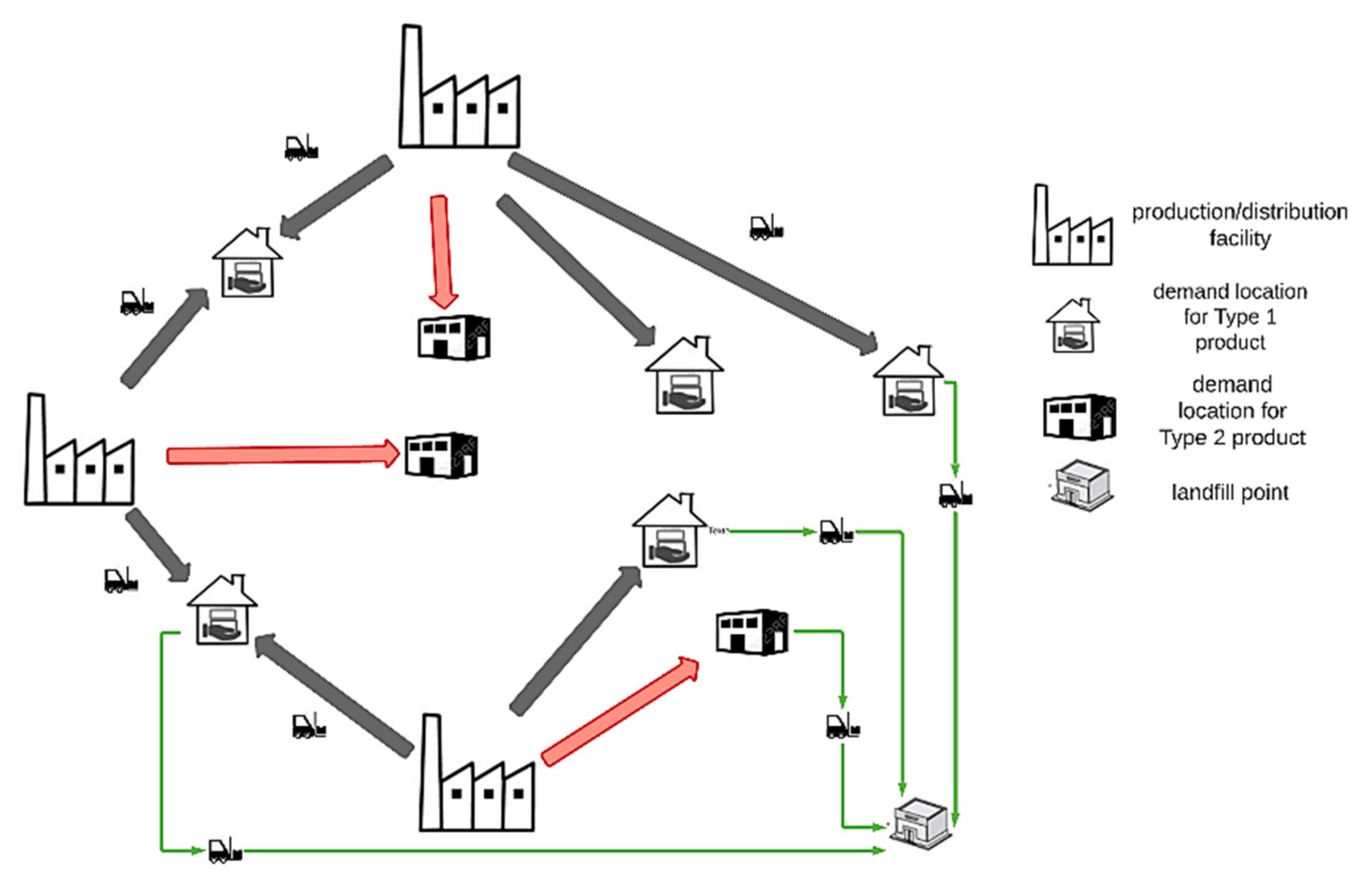
The problem can be explained with the help of Figure 2. The management considers several possible options for deploying their production/distribution facilities. A decision is to be made regarding deploying facilities in the specific locations to optimize the overall effort, i.e., to minimize cost and emissions in delivering products to the respective demand locations. A set of demand locations are available which are distinguished according to the quality of products. For example, the black arrows extending towards the demand location of Type 1 products imply that products with superior quality are transported through this route. The contrary is true for the red arrows extending towards the demand location of Type 2 products. It is worth noticing that multiple-quality products can also be delivered to the same location. Several trucks with heterogeneous capacities are available for transporting products from distribution facilities to demand locations. Since the capacity of trucks vary, a pre-sorting approach is used to take maximum advantage of the available truck capacity. This is done by packing products in boxes which are later loaded into the truck. Products are to be delivered in a time window and the inability to do so will incur penalty.
An illustrative example is produced in Table 2 to explain the modalities of the analysis. There are three types of products (P1–P3) which are to be delivered using two heterogeneous trucks (K1 and K2) to five destination points (J1–J5) in the required quantity of demand. Each product has a specific size with respect to the packaging box which will help in pre-sorting and loading products into the trucks. A time window is available in which the multi-quality and multiple products are to be delivered to the specific locations. It is to be noted that Table 2 only explains the different facets of data and the sample data is offered in the results section. The sample data uses 10 small and 10 large sets of problems using exponential and uniform distribution where a problem size is defined by Cp-i–j (C = problem, p = product type, i = distribution point and j =demand location).
Two strategies are adapted for ensuring the potency of delivered products. These strategies are monitoring strategy and conformity strategy. The monitoring strategy is used to keep the condition of products in check during delivery. Products are distinguished with respect to their state of quality. The bad-quality products can further deteriorate due to perishability, emissions, imperfect refrigeration, and longer travelling distance. Such failing products are separated from the improved quality products and are taken to the landfilling point where they are disposed. In other words, a portion of delivered products are no more needed by customers and they are taken to the landfill sites. It is to be noted that landfilling is performed only in monitoring strategy. It is a less expensive strategy compared to the conformity strategy; however, it has a drawback of not meeting customer’s demand due to the removal of bad-quality products. Thus, extra product units might be needed to meet demand.
The conformity strategy does not monitor the quality of products during the transit, rather, it processes all products to the level of optimal quality at the end. It means that the existing quantity of products can be used and there is no need to acquire extra products to meet the level of demand. However, this strategy is more expansive as it uses chemicals and industrial techniques to process all products. The analysis is carried out to (i) optimize the value of objective functions, (ii) select the number and locations of facilities, (iii) deliver multiple-quality products and iv) analyze the impact of conformity versus monitoring strategies. The model notations are provided in Table 3.
The proposed model contains two objective functions, i.e., the total cost (TC) and the energy emissions (EE). The goal is to select a cold-chain distribution network which minimizes the values of these objective functions. The objective of TC contains the functions of fixed vehicle cost (VC), transportation cost (TRC), penalty cost (PEC), conformity cost (CC), monitoring cost (MC), emission cost (EC) and fuel consumption cost (FC). These functions are given below.
T C = V C + T R C + P E C + C C + M C + E C + F C
V C = k t i d c j d l p p n x i j k p × n t j k × c v k
T R C = k t i d c j d l p p n x i j k p × n t j k × d d i j × u c t k + k t i d c j d l p p n x i j k p × n t j k × e c d + k t b n b p p n y k b × n l p × t r f p
P E C = k t b n b p p n y k b × n l p × p c l f + b n b k t i d c j d l p p n x i j k p α k b m a x e j a t j k , 0 + β k b max a t j k l j , 0 × n b i j b
C C = b n b k t i d c j d l p p n z k b × n b i j b × c c p
M C = k t b n b y k b × f c v + j d l i d c k t b n b y k b × n b i j b × d c v × d d i j
E C = k t i d c j d l p p n x i j k p × n t j k × d d i j × c e k
F C = k t i d c j d l p p n x i j k p × n t j k × d d i j × τ × δ k
Equation (1) presents different components of the TC model. Equations (2)–(8) offers the mathematical functions of different cost components. Equation (2) contains the fixed VC of using number of trucks k. Equation (3) offers transportation cost to demand location, driver exploitation cost and transportation cost to landfill locations. Equation (4) contains the penalty cost due to landfill products and the arrival related cost. The arrival time ( a t j k ) is calculated using the information of distance and vehicle speed between locations. Equation (5) contains the CC if the conformity inspection is used. Equation (6) contains the fixed and variable costs if the monitoring inspection is used. Equation (7) offers the cost of emission due to travelling and Equation (8) provides the expression for fuel consumption.
Equation (9) presents the objective function of EE. The first expression calculates the emissions generated by truck. The second expression calculates emissions due to spoilage of products. The spoilage rate as defined by Wang et al. [40] is 1 e θ p t × 100 % and it varies for different products in the considered case. The deterioration in quality of different products is thus obtained as 1 q p ( 1 e θ p × d d i j v i j ) . Products are in different states of quality which is demonstrated by the index q p . Its value varies between 0–1 where a value closer to zero refers to a bad-quality product and a value closer to 1 refers to a perfect-quality product. A perfect-quality product will have no spoilage ( θ p   = 0) and as the condition of quality deteriorates, the spoilage rate will increase accordingly. The third expression provides emissions due to unloading and waiting at the demand location.
E E = k t i d c j d l p p n x i j k p × n t j k × d d i j × e g k + k t i d c j d l p p n x i j k p × 1 q p ( 1 e θ p d d i j v i j ) × p × n b i j b + k t i d c j d l p p n x i j k p ( u t p j × + γ m a x e j a t j k , 0 ) × n b i j b
The list of constraints is provided by Equations (10)–(20). Equation (10) is used to calculate the number of boxes required for transportation. Equation (11) calculates the number of trucks needed to meet the required demand. Equation (12) calculates the number of landfilled products due to spoilage. Equation (13) ensures that either the monitoring or conformity strategy is adapted at a time. Equations (14)–(16) are truck capacity, distribution center capacity, and demand-related constraints, respectively. A particular customer location is to be visited only once (Equation (17)). Equation (18) provides the time-window constraint. Lastly, Equations (19) and (20) provide the binary and non-negativity constraints, respectively.
n b i j b = b n b j d l p p n h j p × s p × d j p c b b
n t j k = b n b k t i d c j d l p p n x i j k p × n b i j b t c k
n l p = y k b × 1 q p ( 1 e θ p d d i j v i j ) × ω p × n b i j b × c b b s p   ; i = 1 , 2 d c   j = 1 , 2 , d l ,   b         = 1 , 2 , n b ,   k = 1 , 2 . t
m k b = y k b + z k b ;   b = 1 , 2 , n b ,   k = 1 , 2 , t
n b i j b × c b b n t j k × t c k ;   i = 1 , 2 , d c ,   j = 1 , 2 , d l ,   b = 1 , 2 , n b ,   p = 1 , 2 , p n
j d l i d c n b i j b × c b b s p i d c c a i p ;   p = 1 , 2 , p n
j d l i d c n b i j b × c b b s p j d l d j p ;   p = 1 , 2 , p n
p p n k t i d c x i j k p = 1 ;   j = 1 , 2 , d l
e j a t j k l j
x i j k p , y k b ,   z k b     0 ,   1
n t j k ,   n l p 0
Some of the objective functions contain the product of two variables which causes non-linearity. A linearization approach was used for diminishing the non-linear aspects. Table 4 contains the general form of non-linear product of variables B and C which is linearized using an auxiliary variable A and a big number Z. The remaining non-linear relationships are similarly linearized.
The following assumptions are considered for simplifying the model: (i) the geographical locations of different distribution and demand points are known in advance, (ii) all trucks have the same capacity (in the homogeneous fleet case) which is to be respected by the solution, (iii) the traffic related bottlenecks are assumed to be minimum, (iv) a particular demand point can be visited only once, (v) the greenhouse gases are only due to emission of CO2 and (vi) the demand of each product type is to be met in the same period.

3.1. Solution Approach

This study develops the sustainable distribution design of cold-chain products which falls in the category of non-polynomial hard (Np-hard) problems, due to their complexity. The complexity of the presented model in this study is due to the involvement of multiple products, list of available distribution points and several customer locations. These problems cannot be solved using the exact solution approaches, especially when the problem size is large. Thus, meta-heuristics and non-exact approaches are normally used due to their computational efficiency. This study uses two meta-heuristics, i.e., an adapted version of NSGA-II and SPEA-II, and they are discussed in the following sub-sections.

3.1.1. Adaptive NSGA-II (aNSGA-II)

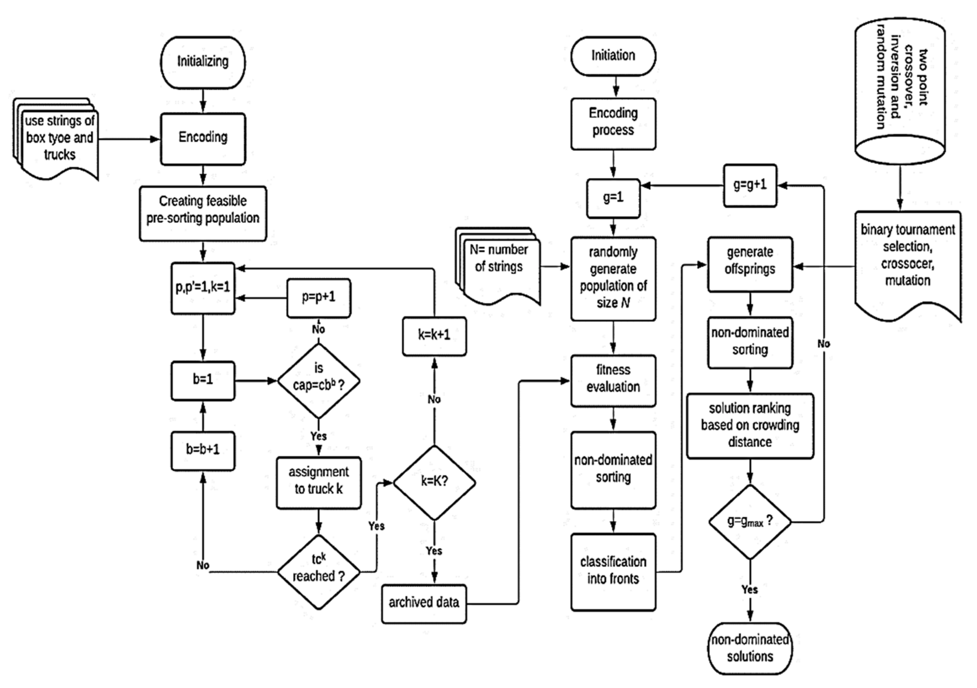
The genetic algorithm (GA) was proposed by Holland [41] and it is inspired by the biological process of evolution. It mimics the behavior of survival of fittest genes in a chromosome and helps in attaining optimal solutions. The NSGA-II is an improved version of GA and it works on the principle of non-domination. It converges multiple objectives to a single fitness function using different fronts which makes it superior to GA. NSGA-II represents the solution as a chromosome and considers parent chromosomes to obtain the offspring. It is applied as a solution approach to the current problem in two inter-related phases. The first phase is a pre-sorting phase, and the second phase is related to assigning truckload between points i (distribution) and j (destination). In the pre-sorting phase, the information of number of product types and their demand, number of boxes, and number of trucks are used as an input to take maximum advantage of the available capacity. Once the pre-sorting is performed, assignment considers the following questions: (a) what is the total number of trucks needed to dispatch the required product quantity? (b) which distribution centers are to be used for dispatching trucks to optimize the bi-objective model? (c) what is the impact of a particular strategy on the potency of delivered products?
The framework of adaptive NSGA-II (aNSGA-II) is provided in Figure 3. The left block is related to pre-sorting and the right block is the main loop of NSGA-II. The pre-sorting works on optimizing the number of boxes in a truck according to the level of demand. In doing so, product dependency is checked (if multiple products are needed at a particular destination) and their sorting is performed. The goal here is to optimally exploit the capacity of available boxes and trucks. This analysis is repeated up until all trucks are filled according to the level of demand of different products and the information is archived. The main loop of algorithm contains the steps of population initiation, generations, solution representation, fitness evaluation, crowding distance sorting, genetic operators, selection strategy, and termination.
The algorithm uses an initial population (Po) to generate the chromosomes. The population size is an important consideration as a small population size will provide inaccurate results and a large population size will take more computation time. A random population of size n is generated to assist in the execution process. The solution representation is performed keeping in view the requirements of different decisions. For instance, a dynamic level of different products demand is needed at different destinations. As shown in Figure 4, three products (p = 3) are demanded by four destination points (J = 4). An entry of zero value means that a product is not needed by the destination. The highlighted demand quantities refer to products which go through monitoring inspection during transportation. For j = 1, products 1 and 3 are to be supplied in quantity of 143 and 230 units with monitoring strategy, respectively.
The chromosome of a typical solution is represented in Figure 5. It is divided into 3 strings for the ease of illustration. The first string contains the repetitive gene values of product information, second string refers to the available distribution points and the third string contains the set of demand locations to be visited. Suppose the analysis is to be carried out for three products (p = 1, 2, 3), four available distribution points (I = 4, 5, 6, 7) and ten destinations (J = 8, 9, 10, 11, 12, 13, 14, 15, 16, 17). The 1st, 2nd, 5th, and 9th components of 1st string belong to product 1 which corresponds to distribution points 4, 6 and 7 and the demand locations 10, 12, 11 and 15 respectively, and so on. One way to look at the available information is to break it down according to the type of products, as shown below.
Product 1: 1-4-12, 1-6-11, 1-7-10-15; Product 2: 2-5-9-14-16; Product 3: 3-4-13-17, 3-6-8
This information can be interpreted in the following way. Product 2 is to be delivered to the demand locations 9, 14, and 16 using distribution point 5. The fitness of solutions is calculated based on the non-domination. For two solutions ×1 and ×2, the non-domination can be explained as follows. The solution ×1 dominates ×2 solution if, (i) ×1 is not worse than ×2 in all objectives and, (ii) ×1 is improved compared to ×2 in at least one of the objective functions. A tournament selection criterion is applied which uses the crowding distance sorting. The crowding distance informs on how much a particular solution is crowded with other solutions. It helps in identifying the number of solutions around a particular solution. The study of Deb et al. [42] can be referred to for more details on the crowding distance sorting.
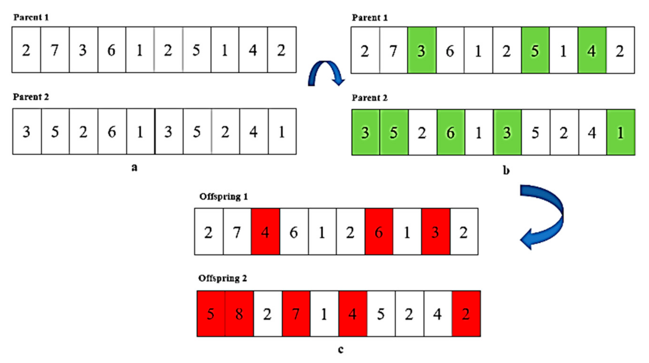
The algorithm uses the genetic operators of crossover and mutation along with the tournament selection to generate fresh offspring. Two parent chromosomes are selected at random and they are treated through the genetic operators to obtain offspring. This study selects a higher crossover rate as the objectives of cost and emissions have a higher correlation. The crossover and mutation operators ensure the convergence and diversity of solutions and both needs to be well balanced. A two-point crossover was used in the current study and its implementation is demonstrated through Figure 6. A pair of parent chromosomes is generated at first and it is cut at two points. The genes within the bounds of the cut points are exchanged between the resulting offspring. The leftover portions of offspring chromosomes remain the same as their respective parents.
The mutation is applied using the inversion and random mutation operators. The application of inversion mutation operator is explained with the help of Figure 7. Two parent chromosomes of length equal to 10 genes are randomly created. Each chromosome is cut at randomly selected two points and the order of genes in the selected portion is inverted. In this way, a pair of offspring is obtained which is later merged with the parent population.
The second mutation operator is based on the random mutation. It works on the following principle: (i) identify the mutation rate (m), (ii) identify the number of genes (nG) to mutate (nG = m × rows × columns), (iii) randomly select genes for mutation, (iv) replace the values of selected genes by random numbers. This procedure is explained with the help of Figure 8. Two parent chromosomes each containing 10 genes are selected at random (rows × columns = 2 × 10 = 20), as shown in Figure 8a. For a random mutation rate (m = 0.4), the number of genes to be mutated is equal to 20 × 0.4 = 8. In the next step, a total number of 8 genes are randomly selected from the parent chromosomes for the process of mutation, as highlighted in Figure 8b. These values are replaced by random numbers resulting in a pair of offspring (Figure 8c).

3.1.2. SPEA-II

Strength pareto evolutionary algorithm (SPEA-II) is an effective technique which reports the non-dominated solutions by identifying the strength of solutions closer to the top ranked solution. It preserves the pareto optimal solutions in an archive using the selection procedure of merging offspring, fitness calculation, tournament selection, and mating. The steps of SPEA-II are given in the following and its pseudocode is provided in Appendix A.
Step 1: Define the population size, archive size, and probabilities of crossover and mutation operators. The algorithm starts by defining and creating an empty archive. It also creates an external archive where the top solutions are stored.
Step 2: The fitness functions of archive and population are calculated. The fitness value is based on non-domination, i.e., for two solutions x and y, the following will hold true.
i 1 , 2 , n :   f i x f i y   a n d j   1 , 2 n :   f j x f j y
Step 3: The non-dominated solutions are copied from the population to archive. As the archive size is pre-defined and limited, truncation is used for removing the excessive solutions.
Step 4: A binary tournament selection is used for creating the offspring. Like NSGA-II, SPEA-II also uses two-point crossover and inversion and random mutation operators for the creation of offspring.
Step 5: The solutions are returned according to the termination criteria of the FI and the BI. The similarity between both algorithm (in terms of crossover, mutation, and termination) is ensured so that both can be compared under similar conditions.
Two search mechanisms are applied as a termination criterion, i.e., the FI and the BI. The FI refers to a situation where solutions are returned when the first improvement in respective values is found and BI returns the solutions when no further improvement in possible. Thus, the analysis is carried out using four variants of algorithms, i.e., SPEA(FI), SPEA(BI), aNSGA-II(FI) and aNSGA-II(BI). To compare the performance of these variants under different problem sizes, two metrics were used, i.e., inverted generational distance (IGD) and hypervolume metric (HyV).
(a)
The IGD calculates the uniformity and solution quality of approximate pareto front (AF) by considering the distance between a real pareto front (RF) and an approximate pareto front (AF). It performs the calculation by using the Euclidean distance approach between RF and AF. The relationship for IGD is provided in (22) where d R F a ,   A F   is the measure of Euclidean distance.
I G D A F ,   R F = a F d R F a ,   A F / R F
(b)
The hypervolume value (HyV) is an estimate of the covered space size. The space size is calculated between an approximate pareto front (AF) and a reference point defined by z. Its relationship is given in (23). The set z = z 1 , z 2 z s   constitutes the value of reference points which are dominated by the respective approximated fronts, s is the number of objective functions and V is the measure of Lebesgue. The first two terms of HyV (AF) relationship are used in this study as it there are two objective functions (i.e., s = 2)
H y V A F = V ( U a A F f 1 a ,   z 1 × f 2 a ,   z 2 × × f s a ,   z s
A value of d R F a ,   A F   = 0 is ideal as it means that AF = RF, i.e., the approximated pareto front is a real solution. Thus, such solutions will have a good convergence. On the other hand, a higher value of HyV is preferred as it reflects better distribution and improved diversity in solutions. A solution approach with minimum IGD and maximum HyV values will be preferred.

4. Results and Discussions

Results

The model was divided into different variants for the purpose of comparison. Three different variants (each containing two classes) were defined according to the vehicle type, product quality, and inspection. Vehicle types were heterogeneous (HeV) and homogeneous (HoV) vehicles. The former contained vehicles with different characteristics and the latter was based on similar vehicle characteristics. The difference between vehicles in the heterogeneous variant is mainly due to the capacity for product boxes, costs, and emissions. The product-quality dimension considered perfect-quality (PQ) and different-quality (DQ) products. The two inspection strategies, i.e., monitoring and conformity, were considered one at a time (Equation (13)), leading to the monitoring only (Mo) and the conformity only (Co) strategy.
A random set of data was generated as there was no available dataset related to multiple products with different states of quality. The suggested approaches and mathematical models were applied to such randomly generated sets of data. In this regard, 10 small and 10 large sets of problems were defined using exponential and uniform distribution. The problem size was defined by Cp-i–j, where C denotes the problem, p is for the number of product types, i is the available list of distribution points and j denotes the set of demand locations. The number of product types in the small-problem instances was defined by U [2; 6] and its distribution for the large problems was defined by U [7; 18]. The number of available distribution points were 5 and 8 and the number of customer destination points were 25 and 40 for the small and large problem sizes, respectively.
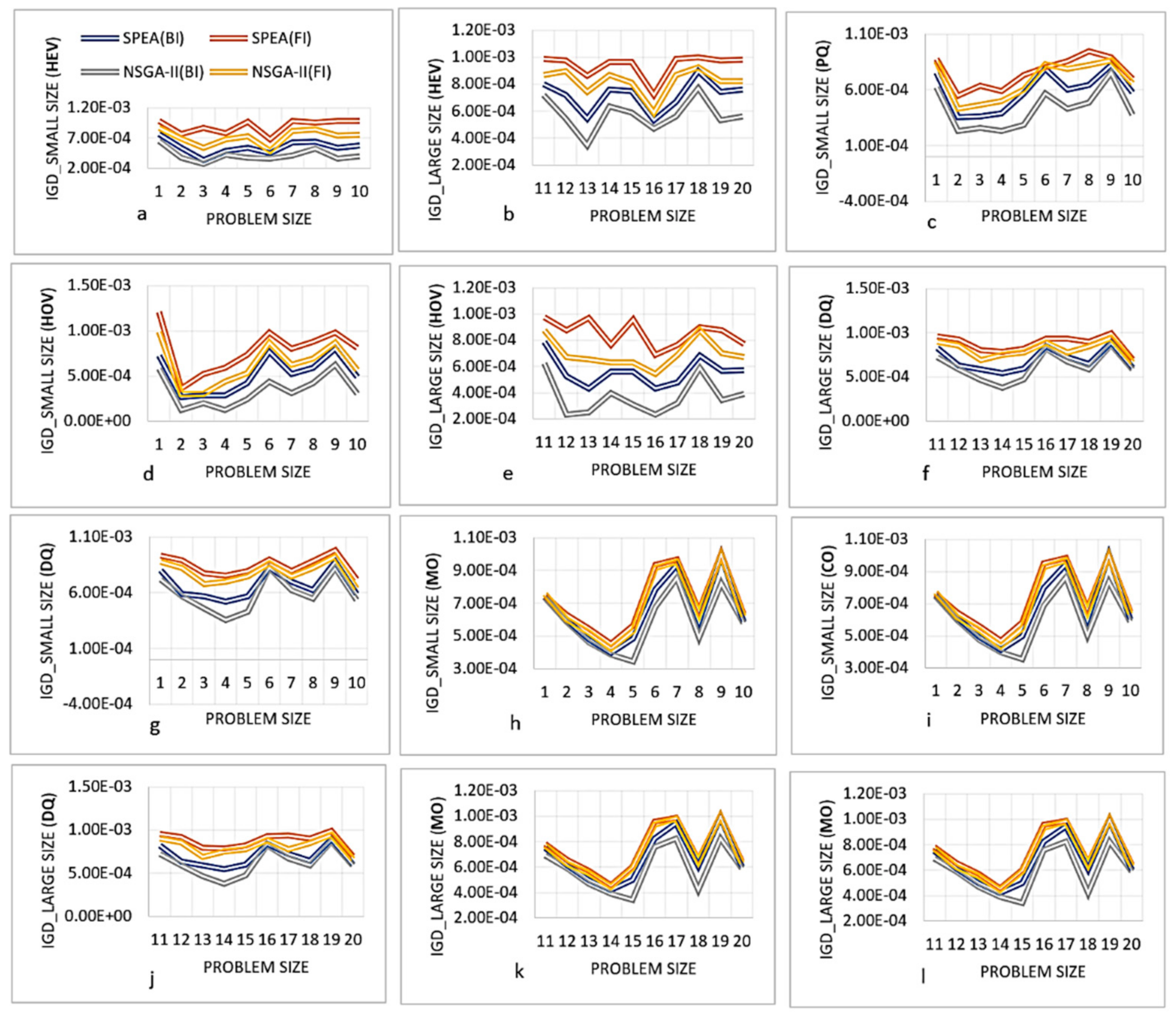
The model was implemented on the generated data using aNSGA-II and SPEA-II. The input parameters of any algorithm are important as they can impact its effectiveness. This study used the population size = 100 for NSGA-II and population size = 80 and archive size = 25 for SPEA-II. Both algorithms were assigned the similar crossover and mutation values, i.e., crossover = 0.6 and mutation = 0.3, and binary tournament was used as the selection criteria. The model was coded in MATLAB 2014a on a Core i5 system, 2.8 GHz and 8 GB RAM. Initially, the four variants of algorithms, i.e., SPEA (BI), SPEA (FI), NSGA-II (BI) and NSGA-II (FI), were tested using small and large problem instances to compare their HyV and IGD scores. The iteration size was kept 20 and the HyV and IGD scores are provided in Figure 9 and Figure 10, respectively.
The following implications can be drawn from both figures:
(a)
There were no large-scale differences between the results of small and large size problems of a particular variant. Thus, the heuristics are powerful enough to address the complexity of a given problem.
(b)
The termination criteria based on returning solutions after BI works well compared to FI. BI is a more exhaustive search mechanism which seeks stability and refinement of solutions before returning them.
(c)
The adaptive NSGA-II (BI) has the standout scores of HyV and IGD for all test cases, ensures better uniformity and convergence of solutions; however, it took more time due to the pre-sorting.
(d)
The HyV and IGD scores of Mo and Co strategies are somewhat similar in small- and large-scale problems; however, this aspect will be further examined with the help of a detailed analysis of cost.
(e)
The homogeneous (HoV) and PQ distributions are favored as they have improved scores compared to the scores of heterogeneous (HeV) and DQ products-based analysis. This might be because such aspects pose less complexity in computation and hence the model performs well in such cases. Based on the presented analysis, NSGA-II (BI) was selected to carry out further analysis due to its improved performance.
A particular case, i.e., C4-5-25, was examined to understand the different modalities. The goal was to analyze the effectiveness of distribution points in minimizing cost and emissions using the key factors of quality differentiation and perishability. In a first, the analysis assists the management in examining the role of different inspection strategies during distribution. The problem involves five possible distribution centers (I1 to I5), four product types (p1, p2, p3 and p4) which are to be transported in different combinations to 25 distribution centers. The data related to demand locations, product requirement, quantity of demand, co-ordinates, and time window of delivery is provided in Table 5. The demand quantities of product 1, 2, 3 and 4 are 3825, 3020, 1605, and 3385 units, respectively. Table 6 contains the data related to different distribution centers. Table 7 and Table 8 contain the data related to parameters of trucks and input parameters of the model, respectively.
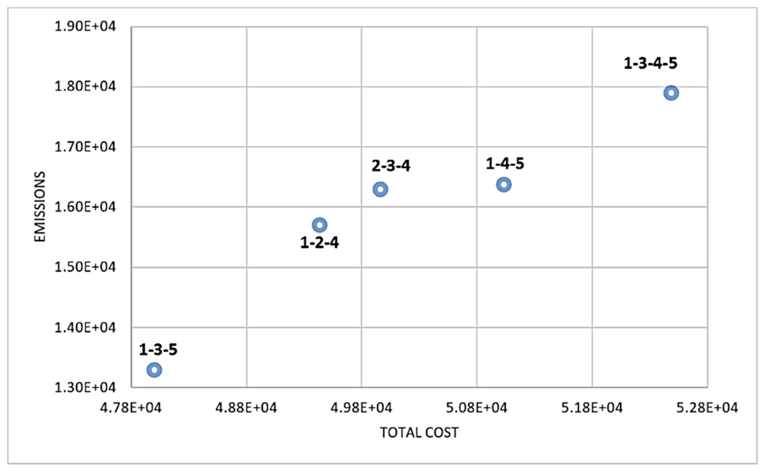
A list of non-dominated solutions is generated once the model is implemented. These solutions are non-dominated due to the trade-off between cost and emissions and the use of different combination of distribution points. Some of the non-dominated solutions are provided in Figure 11. Clearly, different distribution centers yield different results. Some of these results are better on the dimension of cost and some show an improved performance against emissions. The combination of distribution centers 1-3-5 can be a global solution as it performs equally well on the dimensions of cost and emissions. It can be observed that the value of cost increases by increasing the number of distribution points. The geographical location of a distribution point regarding the density of destination points affects the decisions of cost and emissions. For example, in Figure 11, between two solutions (1-3-5 and 1-4-5), there is a difference of only one distribution point; however, it affects the objective functions to a larger extent and results in almost 20% increase in cost and emissions.
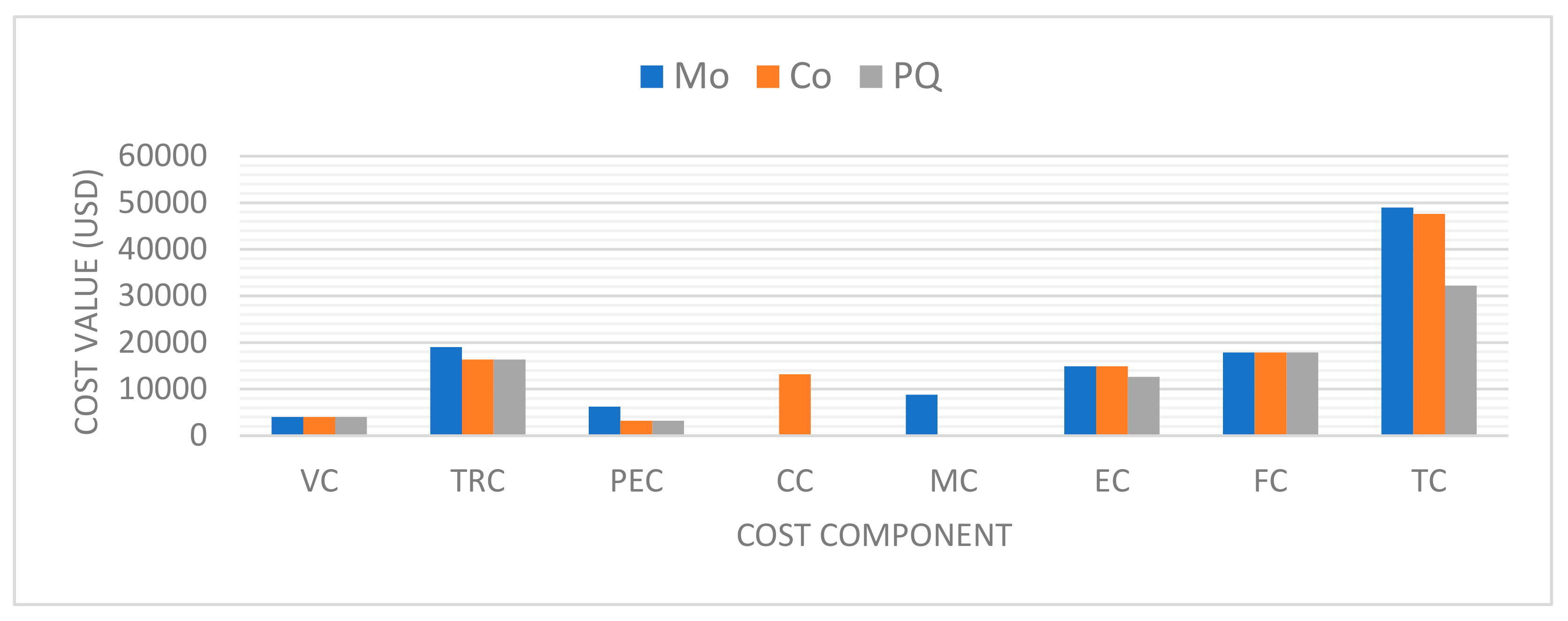
The comparison of different components of minimum cost solution (1-3-5) according to monitoring only (Mo), conformity only (Co) and PQ situations is provided in Figure 12. The following conclusions can be drawn:
(a)
The TC value is minimum when products are in perfect quality. It is because there are no costs related to conformity and monitoring inspection. Also, transportation and emission costs are lower in this case as there are no landfilled products and hence no need to transport the bad products to the landfilled points.
(b)
The conformity inspection performs better compared to the monitoring inspection in the presence of quality issues and it results in almost 2% less cost.
(c)
A higher value of TC in the monitoring only strategy is due to the higher transportation and penalty cost. It segregates the bad-quality products and sends them to the landfill point which results in higher transportation and penalty cost.
(d)
As established earlier, conformity is an expensive strategy, and the results show that the CC is $13,175 which is almost 50% higher than the MC ($8825). However, this difference is discounted by the costs of transportation and penalty of bad products in the monitoring strategy.
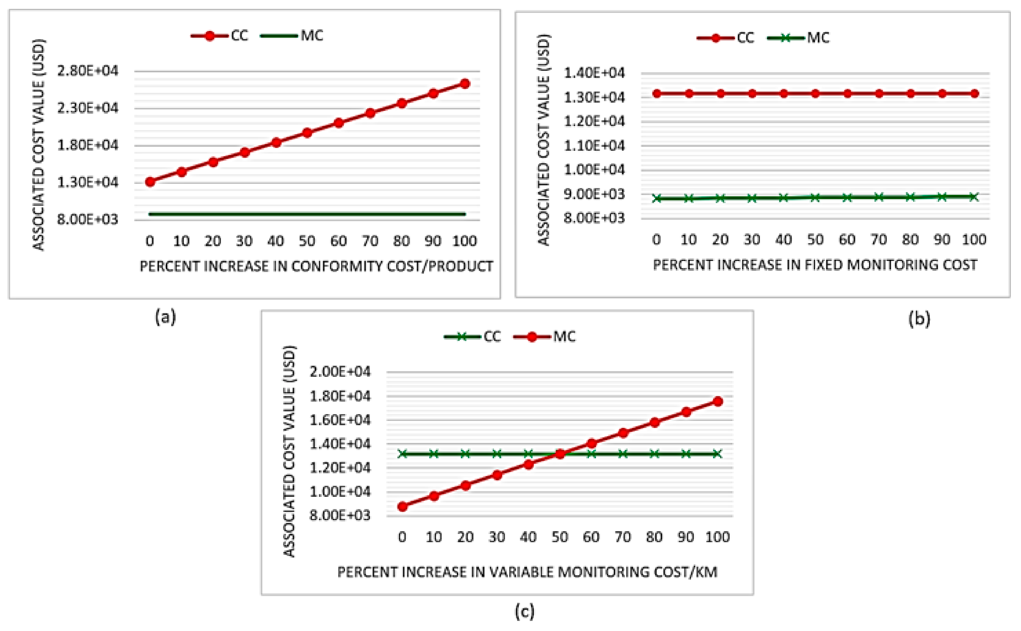
The conformity and monitoring analysis are dependent on the characteristics of product, fixed cost of monitoring, and distance travelled. A complex or delicate part may involve a higher cost of conformance. Similarly, the MC will be higher for transportation to a distant location. Thus, it is beneficial to perform a comparison between both strategies subject to changing values of cost. Figure 13 presents the results of sensitivity analysis of different strategies. Figure 13a presents the sensitivity analysis of MC and CC subject to percent increase in conforming cost. It can be observed that the CC is always higher, and it linearly increases. As the percentage increase goes up, the difference between CC and MC further enhances. Figure 13b presents the sensitivity between CC and MC when the fixed cost of monitoring is increased. It can be observed that it has almost no impact on diminishing the gap between MC and CC.
The sensitivity analysis between MC and CC regarding changing values of monitoring cost per km is presented in Figure 13c. The difference between CC and MC keeps on diminishing as the percentage increase occurs in the value of monitoring cost/km up until 50% at which point, a breakeven is achieved between MC and CC. As the percentage increase in variable monitoring cost/km goes beyond 50%, monitoring only (Mo) is no more a viable strategy as it costs more. It can be concluded that:
  • Conformity only is not an ideal approach for product-quality assessment during the transit.
  • Changes in fixed MC has least effect on selecting a strategy.
  • The management should pay more attention towards the sensitivity of variable MC as it can alter the decision of inspection strategy at some point.
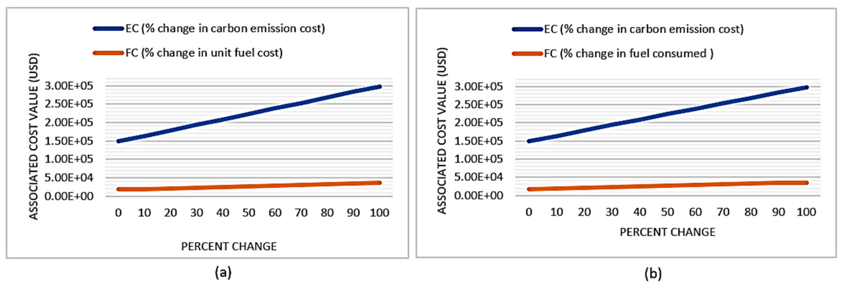
The trucks may consume less fuel (hence less FC and emissions) if they are in working conditions such as new trucks and the road condition is better. On the contrary, if the trucks are in deteriorated condition, they may use more fuel per km. Similarly, government has a pioneering role in regulating the prices of fuel and carbon emission. It has been observed that the fuel prices are more volatile and subject to changes in the underdeveloped countries. To understand the uncertainty of such conditions, Figure 14 provides the results of sensitivity analysis of (i) EC due to the change in carbon emission prices (a, b), and (ii) FC due to the change in unit-fuel cost (a) and due to the change in fuel consumed by truck per km (b). It can be argued from Figure 14a,b that the change in unit-fuel cost and change in fuel consumption per km have relatively less effect on the overall cost solution as compared to the change in the prices of carbon emission. This provides an implication for management when facing the challenge of a trade-off among unit-fuel cost adjustment, fuel consumption, and the cost of carbon emission. Ideally all three need to be controlled; however, if management wants to prioritize a particular element, it can control the cost of carbon emission. It is noteworthy that the carbon emission also impacts the second objective function of this study which makes it even more important in terms of enhancing the efficiency of cold-chain distribution.
The link between emissions and financial performance has been explored by many authors and it is a well-established area of research. In the earlier publications, it was argued that companies committed to environment anticipate a decrease in their financial performance as they shift their focus from the hard-core profit aspects to the softer issues of sustainability and preserving the environment [43,44]. A different perspective has also evolved which argues that companies involved in environmental sustainability possess tacit knowledge and techniques which are difficult to imitate, thus, they are able to attain a strategic competitive edge over their competitors and it is rewarding to be green [45]. Indeed, according to the triple-bottom-line approach, emissions and cost decisions are closely linked. Another dimension that links costs and emissions, as described by Coronella et al. [46], is conducting businesses according to the ethical and corporate social responsibility (CSR) values. Thus, the short- and long-term business goals are aligned with the well-being of the community. To this end, the findings of this study reinforce the notion that a sustainable distribution design will offer a balance between cost and emission and CSR responsiveness. The managers may find the role of inspection strategy, selection of a distribution point, quality conditions of different products and their perishability and sensitivity of different model aspects interesting in taking a strategic lead and becoming more sustainable and responsible towards preserving the environment and maximizing profit.

5. Research, Managerial, and Policy Implications

This study presented a bi-objective model for optimizing cost and emissions in a cold chain. The distribution system was based on multiple products with different quality conditions. The model was implemented on a case study using pre-sorting embedded with NSGA-II and SPEA-II. The study contains the following implications for managers and practitioners.

5.1. Research Implications

  • This study implemented two algorithms with different termination criteria. The termination criterion based on the BI works well and NSGA-II (BI) has the best values of IGD and HyV in all test problems. It can be interesting to validate the findings using NSGA-II (BI) with and without the pre-sorting.
  • There were no significant differences between the results of small and large problem sizes of a particular model variant. This indicates the robustness of the solution approaches. Furthermore, the model worked well in the absence of an additional scale of complexity.
  • The geographical location of a candidate distribution point regarding the density of destination points impacts the solutions. A careful selection of a distribution point is imperative as it can influence the cost and emissions of the distribution system. In other words, the objective function values are sensitive to minor changes in the combination of distribution points. In this regard, minor changes can amount to higher differences in the values of objective functions.

5.2. Managerial and Policy Implications

  • A thoughtful selection of distribution centers is imperative as it affects the objective functions of cost and emissions. A distribution network of PQ products is always advantageous in obtaining the lower values of cost and emissions; however, it is not always practical. The real-life situations contain products in different states of quality. Thus, managers can examine the quality of products prior to dispatching so that an optimal decision can be made. The state of quality of products can be recorded along with the data of cost, time, and emissions. Such information will offer an enabling approach to sustain the perishability and usefulness of products for customers by delivering products in optimal quality.
  • The problem addressed in this study can be appealing to the underdeveloped countries where imperfect refrigeration, energy shortfall, and the inability to deliver products responsively are more pertinent issues. The model and its implications are applicable to the distribution of vaccines, ice-creams, and medicines. The vaccines in particular needs a more controlled transportation mechanism as they have a limited shelf life. A long transportation route, quality deterioration, or an imperfect refrigeration can result in the expiry of vaccines. Since the demand of vaccines for the epidemic diseases is more in the underdeveloped countries, the presented findings may assist the policy makers in assessing how quality deterioration may impact the overall costs and emissions of distribution centers.
  • Managers can adapt one of the two strategies, i.e., monitoring or conformity strategy, to ensure that higher quality products reach to the customers. Adapting any of these strategies depends on the data related to cost, distance etc. Our results show that the conformity strategy is a more viable option as it results in less cost as well as it delivers all products to the destination points. Compared to it, monitoring strategy landfills the bad products which decreases the quantity of delivered products.
  • The monitoring only (Mo) is an expensive strategy as it has higher transportation and penalty costs. The MC is more sensitive towards changes, as compared to the CC; however, management should pay attention towards change in the parameters of CC (as higher rate of changes can impact the decision of selecting a strategy).
  • Experience shows that a product in damaged state can seldom be repaired to a state as good as new. Thus, if customer satisfaction is prioritized rather than cost, a manager may opt for monitoring strategy as it is not concerned with delivering products which have issues related to quality.
  • There is more perishability if a product is in bad condition of quality. This can enhance the chances of product failure and landfilling. To avoid this, higher transportation speeds can be used for a responsive delivery. Though this practice may deliver products before large-scale quality disruptions, higher speed of delivery can cause an increase in emissions. Thus, a careful analysis of quality condition, perishability, and delivery speed is needful on the part of manager.
  • The cost of carbon emission needs to be controlled as it impacts the objective functions of cost and emissions. The results showed that the importance of carbon emission surpassed the need to control fuel price and fuel consumption per km. However, these findings are in light of developed economies where fuel prices undergo minor revisions. A different result might be anticipated in underdeveloped economies where fuel prices undergo major revisions.

6. Conclusions

The distribution of cold-chain products is a challenging task as it involves time-sensitive and perishable products. Any delay in product delivery can impact the product usefulness, cost efficiency, and emissions. This study considered the distribution system of multi-quality multiple-cold-chain products. A bi-objective model of cost and emissions was proposed and implemented using two meta-heuristics. The results presented a comparison between different inspection strategies, quality conditions, and different components of cost.
Although different factors of cold-chain distribution were analyzed; however, this study has certain limitations which are provided as following. The model considered a deterministic behavior of perishability and quality conditions. It will be interesting to analyze the dynamic and fuzzy behavior of such aspects to make the model more practical. The traffic, road conditions, weather-related aspects, and driver fatigues were not directly considered. Modelling such aspects will further provide interesting implications. This study assumed that the demand locations are known in advance. However, in the distribution of the cold chain such as in emergency response in healthcare, the level of demand may not be known in advance. This aspect may reduce the scope of application of the findings to the health care sector. Furthermore, besides CO2, emissions are caused by various other gases which were not considered in this study.
The following constitutes the guidelines for future research. The presented framework is generalized, and it can be applied to multiple contexts. Research shows that emissions are related to and can be controlled by using policies such as the carbon cap and trade. Future research can examine inspection strategies under the carbon cap and trade policy to understand which strategy performs well. The results can be compared by using other algorithms. Such comparison is a standard practice in the literature where the computational efficiency of solution approaches is tested. The results of the proposed approach can be compared with bee’s algorithm and ant colony optimization.

Author Contributions

Conceptualization, A.S.K. and B.S.; Methodology, A.S.K. and R.K.; Supervision, B.S. and D.Z. and C.I.P.; Formal Analysis, M.I.; Validation, D.Z.; Guidance, C.I.P.; Writing Original Draft, R.K.; Funding Acquisition, B.S. All authors have read and agreed to the published version of the manuscript.

Funding

This study received funding from King Saud University, Saudi Arabia through researchers supporting project number (RSP-2020/145). In addition, if accepted, the APCs will funded by King Saud University, Saudi Arabia through researchers supporting project number (RSP-2020/145).

Acknowledgments

The authors extend their appreciation to King Saud University, Saudi Arabia for funding this work through researchers supporting project number (RSP-2020/145).

Conflicts of Interest

The authors declare no conflict of interest.

Appendix A

Pseudocode of SPEA-II
Define: Size of population, size of archive, crossover, and mutation probabilities
Initialize the population
Define an empty archive
For i = 1−size of population
Calculate the fitness function values of population and external archive
Copy all pareto fronts from population to archive
If pareto fronts > capacity of archive do
Perform truncation
Apply tournament selection and genetic operators
Add solutions to the external archive
End for

References

  1. Sinha, A.K.; Verma, A.R.; Chandrakar, A.; Khes, S.P.; Panda, P.S.; Dixit, S. Evaluation of cold chain and logistics management practice in drug district of Chhattisgarh: Pointer from central India. Int. J. Community Med. Public Health 2017, 4, 390–395. [Google Scholar] [CrossRef] [Green Version]
  2. Fan, J.; Li, J.; Wu, Y.; Wang, S.; Zhao, D. The effects of allowance price on energy demand under a personal carbon trading scheme. Appl. Energy 2016, 170, 242–249. [Google Scholar] [CrossRef]
  3. Mercier, S.; Villeneuve, S.; Mondor, M.; Uysal, I. Time-Temperature Management Along the Food Cold Chain: A Review of Recent Developments. Compr. Rev. Food Sci. Food Saf. 2017, 16, 647–667. [Google Scholar] [CrossRef]
  4. Fera, M.; Fruggiero, F.; Lambiase, A.; Macchiaroli, R.; Miranda, S. The role of uncertainty in supply chains under dynamic modeling. Int. J. Ind. Eng. Comput. 2017, 8, 119–140. [Google Scholar] [CrossRef]
  5. Wang, S.; Tao, F.; Shi, Y. Optimization of Location–Routing Problem for Cold Chain Logistics Considering Carbon Footprint. Int. J. Environ. Res. Public Health 2018, 15, 86. [Google Scholar] [CrossRef] [PubMed] [Green Version]
  6. Konur, D.; Campbell, J.; Monfared, S. Economic and environmental considerations in a stochastic inventory control model with order splitting under di_erent delivery schedules among suppliers. Omega 2017, 71, 46–65. [Google Scholar] [CrossRef]
  7. Grace, D. Food Safety in Low and Middle Income Countries. Int. J. Environ. Res. Public Health 2015, 12, 10490–10507. [Google Scholar] [CrossRef] [PubMed] [Green Version]
  8. John, M. Top Markets Report Cold Chain; International Trade Administration, 2016. Available online: https://legacy.trade.gov/topmarkets/pdf/Cold_Chain_Executive_Summary.pdf (accessed on 18 November 2020).
  9. Balamurugan, T.; Karunamoorthy, L.; Arunkumar, N.; Santhosh, D. Optimization of Inventory Routing Problem to Minimize Carbon Dioxide Emission. Int. J. Simul. Model. 2018, 17, 42–54. [Google Scholar] [CrossRef]
  10. Ali, I.; Nagalingam, S.; Gurd, B. A resilience model for cold chain logistics of perishable products. Int. J. Logist. Manag. 2018, 29, 922–941. [Google Scholar] [CrossRef]
  11. Hariga, M.; As’ad, R.; Shamayleh, A. Integrated economic and environmental models for a multistage cold supply chain under carbon tax regulation. J. Clean. Prod. 2017, 166, 1357–1371. [Google Scholar] [CrossRef]
  12. Shamayleh, A.; Hariga, M.; As’Ad, R.; Diabat, A. Economic and environmental models for cold products with time varying demand. J. Clean. Prod. 2019, 212, 847–863. [Google Scholar] [CrossRef]
  13. James, S.J.; James, C. The food cold-chain and climate change. Food Res. Int. 2010, 43, 1944–1956. [Google Scholar] [CrossRef]
  14. Saif, A.; Elhedhli, S. Cold supply chain design with environmental considerations: A simulation-optimization approach. Eur. J. Oper. Res. 2016, 251, 274–287. [Google Scholar] [CrossRef]
  15. Wang, S.; Tao, F.; Shi, Y.; Wen, H. Optimization of Vehicle Routing Problem with Time Windows for Cold Chain Logistics Based on Carbon Tax. Sustainability 2017, 9, 694. [Google Scholar] [CrossRef] [Green Version]
  16. Kazemian, I.; Aref, S. A green perspective on capacitated time-dependent vehicle routing problem with time windows. Int. J. Supply Chain Inventory Manag. 2017, 2, 20–38. [Google Scholar] [CrossRef]
  17. Bozorgi, A.; Pazour, J.; Nazzal, D. A new inventory model for cold items that considers costs and emissions. Int. J. Prod. Econ. 2014, 155, 114–125. [Google Scholar] [CrossRef]
  18. Qin, G.; Tao, F.; Li, L. A Vehicle Routing Optimization Problem for Cold Chain Logistics Considering Customer Satisfaction and Carbon Emissions. Int. J. Environ. Res. Public Heal. 2019, 16, 576. [Google Scholar] [CrossRef] [Green Version]
  19. Li, Y.; Lim, M.K.; Tseng, M.-L. A green vehicle routing model based on modified particle swarm optimization for cold chain logistics. Ind. Manag. Data Syst. 2019, 119, 473–494. [Google Scholar] [CrossRef]
  20. Manikas, I.; Terry, L.A. A case study assessment of the operational performance of a multiple fresh produce distribution centre in the UK. Br. Food J. 2009, 111, 421–435. [Google Scholar] [CrossRef]
  21. Zangeneh, M.; Akram, A.; Nielsen, P.; Keyhani, A. Developing location indicators for Agricultural Service Center: A Delphi–TOPSIS–FAHP approach. Prod. Manuf. Res. 2015, 3, 124–148. [Google Scholar] [CrossRef] [Green Version]
  22. Chen, H.-K.; Hsueh, C.-F.; Chang, M.-S. Production scheduling and vehicle routing with time windows for perishable food products. Comput. Oper. Res. 2009, 36, 2311–2319. [Google Scholar] [CrossRef]
  23. Yi, W.-J.; Zou, L.-L.; Guo, J.; Wang, K.; Wei, Y.-M. How can China reach its CO2 intensity reduction targets by 2020? A regional allocation based on equity and development. Energy Policy 2011, 39, 2407–2415. [Google Scholar] [CrossRef]
  24. GhannadPour, S.F.; Noori, S.; Tavakkoli-Moghaddam, R. Multiobjective Dynamic Vehicle Routing Problem With Fuzzy Travel Times and Customers’ Satisfaction in Supply Chain Management. IEEE Trans. Eng. Manag. 2013, 60, 777–790. [Google Scholar] [CrossRef]
  25. Li, L.; Yang, Y.; Qin, G. Optimization of Integrated Inventory Routing Problem for Cold Chain Logistics Considering Carbon Footprint and Carbon Regulations. Sustainability 2019, 11, 4628. [Google Scholar] [CrossRef] [Green Version]
  26. Drezner, Z.; Scott, C.H. Location of a distribution center for a perishable product. Math. Methods Oper. Res. 2013, 78, 301–314. [Google Scholar] [CrossRef]
  27. Khan, A.S.; Pruncu, C.; Khan, R.; Naeem, K.; Ghaffar, A.; Ashraf, P.; Room, S. A Trade-Off Analysis of Economic and Environmental Aspects of a Disruption Based Closed-Loop Supply Chain Network. Sustainability 2020, 12, 7056. [Google Scholar] [CrossRef]
  28. Mejjaouli, S.; Babiceanu, R.F. Cold supply chain logistics: System optimization for real-time rerouting transportation solutions. Comput. Ind. 2018, 95, 68–80. [Google Scholar] [CrossRef]
  29. Verbič, M. Discussing the parameters of preservation of perishable goods in a cold logistic chain model. Appl. Econ. 2006, 38, 137–147. [Google Scholar] [CrossRef]
  30. Song, M.-X.; Li, J.-Q.; Han, Y.-Q.; Han, Y.-Y.; Liu, L.-L.; Sun, Q. Metaheuristics for solving the vehicle routing problem with the time windows and energy consumption in cold chain logistics. Appl. Soft Comput. 2020, 95, 106561. [Google Scholar] [CrossRef]
  31. Yan, L.; Grifoll, M.; Zheng, P. Model and Algorithm of Two-Stage Distribution Location Routing with Hard Time Window for City Cold-Chain Logistics. Appl. Sci. 2020, 10, 2564. [Google Scholar] [CrossRef] [Green Version]
  32. Qiang, X.; Appiah, M.Y.; Boateng, K.; Appiah, F.V. Route optimization cold chain logistic distribution using greedy search method. OPSEARCH 2020, 57, 1115–1130. [Google Scholar] [CrossRef]
  33. Wang, Z.; Wen, P. Optimization of a Low-Carbon Two-Echelon Heterogeneous-Fleet Vehicle Routing for Cold Chain Logistics under Mixed Time Window. Sustainability 2020, 12, 1967. [Google Scholar] [CrossRef] [Green Version]
  34. Zhao, B.; Gui, H.; Li, H.; Xue, J. Cold Chain Logistics Path Optimization via Improved Multi-Objective Ant Colony Algorithm. IEEE Access 2020, 8, 142977–142995. [Google Scholar] [CrossRef]
  35. Osvald, A.; Stirn, L.Z. A vehicle routing algorithm for the distribution of fresh vegetables and similar perishable food. J. Food Eng. 2008, 85, 285–295. [Google Scholar] [CrossRef]
  36. Ho, W.K.; Ang, J.C.; Lim, A. A hybrid search algorithm for the vehicle routing problem with time windows. Int. J. Artif. Intell. Tools 2001, 10, 431–449. [Google Scholar] [CrossRef]
  37. Zheng, G.; Liu, L.; Deng, L. Location-Routing Optimization of Cold Chain Distribution Center Based on Hybrid Genetic Algorithm—Tabu Search. In Proceedings of the 14th COTA International Conference of Transportation Professionals, Changsha, China, 4–7 July 2014. [Google Scholar]
  38. Wang, S.; Tao, F.; Shi, Y. Optimization of Inventory Routing Problem in Refined Oil Logistics with the Perspective of Carbon Tax. Energies 2018, 11, 1437. [Google Scholar] [CrossRef] [Green Version]
  39. Shen, L.; Tao, F.; Wang, S. Multi-Depot Incomplete Open Vehicle Routing Problem with TimeWindows Based on Carbon Trading. Int. J. Environ. Res. Public Health 2018, 15, 2025. [Google Scholar] [CrossRef] [Green Version]
  40. Wang, M.; Mao, C.; Yang, C.C. Research on cold chain logistics node location based on genetic algorithms. Sci. Technol. Manag. 2009, 11, 6. [Google Scholar]
  41. Holland, J.H. An efficient genetic algorithm for the traveling salesman problem. Eur. J. Oper. Res. 1975, 145, 606–617. [Google Scholar]
  42. Deb, K.; Agrawal, S.; Pratap, A.; Meyarivan, T. A fast-elitist non-dominated sorting genetic algorithm for multi-objective optimization: NSGA-II. In Proceedings of the International Conference on Parallel Problem Solving From Nature; Springer: Berlin/Heidelberg, Germany, 2000; pp. 849–858. [Google Scholar]
  43. Walley, N.; Whitehead, B. It’s not easy being green. Reader Bus. Environ. 1994, 36, 4. [Google Scholar]
  44. Hull, C.E.; Rothenberg, S. Firm performance: The interactions of corporate social performance with innovation and industry differentiation. Strat. Manag. J. 2008, 29, 781–789. [Google Scholar] [CrossRef]
  45. Hart, S.L. Beyond greening: Strategies for a sustainable world. Harv. Business Rev. 1997, 75, 66–77. [Google Scholar]
  46. Coronella, S.; Caputo, F.; Leopizzi, R.; Venturelli, A. Corporate social responsibility in Economia Aziendale scholars’ theories. Meditari Account. Res. 2018, 26, 640–656. [Google Scholar] [CrossRef]
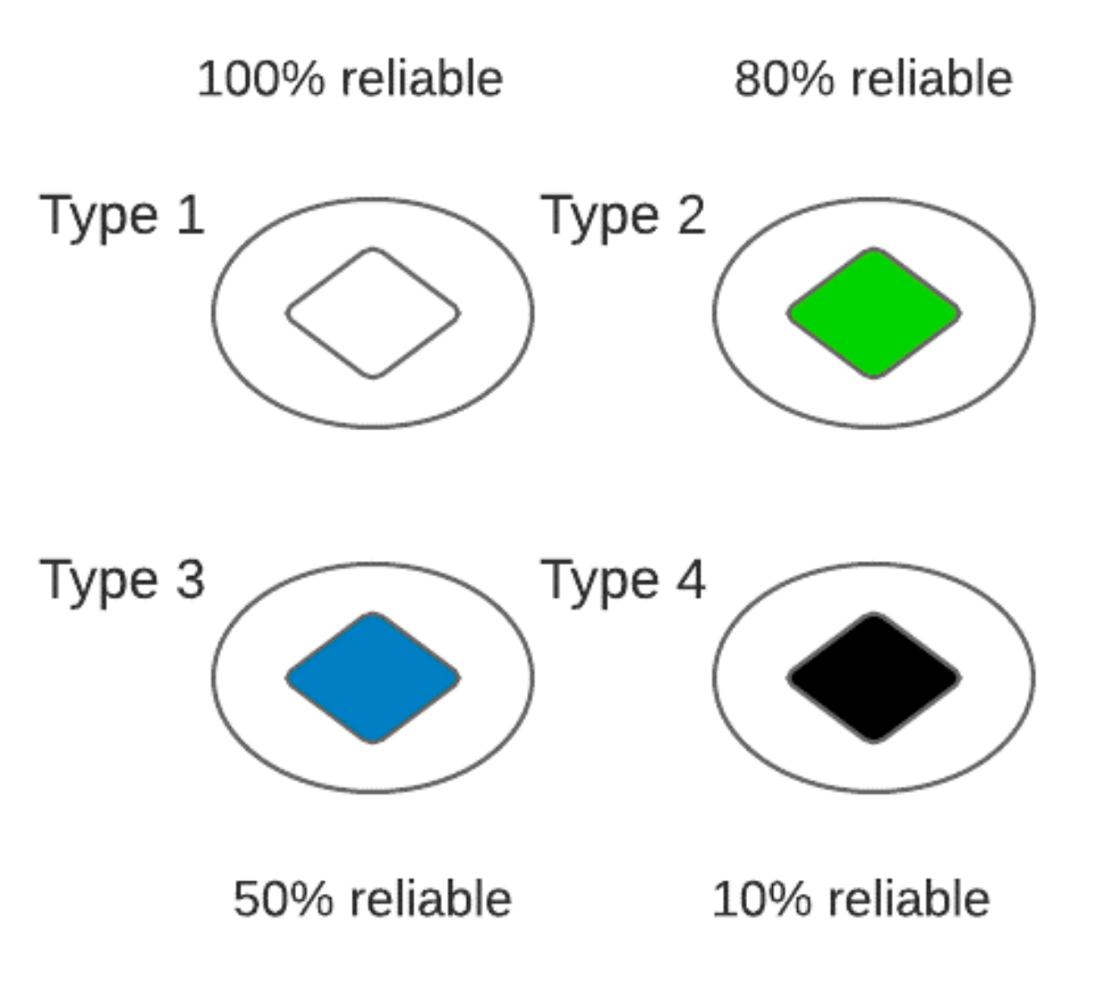
Figure 1. The different states of product quality.
Energies 13 06612 g001
Figure 2. Design of distribution network for multi-quality products.
Energies 13 06612 g002
Figure 3. Framework of adaptive NSGA-II (aNSGA-II) algorithm.
Energies 13 06612 g003
Figure 4. Product demand and destination relationship.
Energies 13 06612 g004
Figure 5. Solution representation.
Energies 13 06612 g005
Figure 6. A two-point crossover.
Energies 13 06612 g006
Figure 7. Inversion mutation operator.
Energies 13 06612 g007
Figure 8. Random Mutation with a pre-defined mutation rate.
Energies 13 06612 g008
Figure 9. Hypervolume (HyV) scores for small and large problem instances of Heterogeneous vehicles (a,b), Homogeneous vehicles (d,e), perfect-quality products (PQ) (c,f), different-quality products (DQ) (g,j), monitoring only (Mo) (h,k) and conformity only (Co) (i,l).
Energies 13 06612 g009
Figure 10. Inverted generational distance (IGD) scores for small and large problem instances of Heterogeneous vehicles (a,b), Homogeneous vehicles (d,e), perfect-quality products (PQ) (c,f), different-quality products (DQ) (g,j), monitoring only (Mo) (h,k) and conformity only (Co) (i,l).
Energies 13 06612 g010
Figure 11. The non-dominated solutions of cost and emissions.
Energies 13 06612 g011
Figure 12. Cost comparison of monitoring only (Mo), conformity only (Co) and perfect-quality products (PQ).
Energies 13 06612 g012
Figure 13. Sensitivity analysis of conformity and monitoring analysis.
Energies 13 06612 g013
Figure 14. Sensitivity analysis of (a) change in emission cost (EC) and change in unit-fuel cost (FC) and (b) change in emission cost (EC) and fuel consumed by truck/km (FC function).
Energies 13 06612 g014
Table 1. The summary of cold-chain literature.
RefYearInspection StrategyEmission AspectsProduct TypesProduct-Quality AnalysisVehicle TypesCost Related to Quality
TEDESingleMultiHoHePCIC
Verbic et al. [29]2006
Wang et al. [15]2018
Mejjaouli et al. [28]2018
Qin et al. [18]2019
Li et al. [19]2019
Li et al. [25]2019
Song et al. [30]2020
Yan et al. [31]2020
Qiang et al. [32]2020
Wang et al. [33]2020
Zhao et al. [34]2020
TE = transportation emissions, DE = deterioration emissions, Ho = homogeneous vehicles, He = heterogeneous vehicles, PC = penalty cost, IC = inspection cost.
Table 2. An illustrative example of the heterogeneous multi-quality multiple-cold-chain distribution.
Customer LocationVehicle TypeProduct TypeSize of Product Regarding Box CapacityDemandTime Window
K1K2P1P2P3P1P2P3P1P2P3[Eij Lij]
J1011000.510.420.3625000[07:10, 09:30]
J2110110300180[06:45, 10:00]
J3101012000220[07:00, 09:45]
J4101101502000[08:10, 10:20]
J50101002650[07:20, 10:30]
Table 3. Description of model components.
NotationDescription
p set of product types   p = 1 , 2 p n
i set of distribution facilities   i = 1 , 2 d c
j set of demand locations   j = 1 , 2 d l
k set of available trucks   k = 1 , 2 t
b set of packaging boxes   b = 1 , 2 n b
d d i j distance between distribution point i and demand location j
c a i p capacity of distribution point for product p
c v k cost of using truck k
c c p conformity cost of product p
u c t k transportation cost of truck k per unit distance covered
e c d exploitation cost of driver
t r f p transportation cost per unit product p to landfilling point
p c l f penalty cost of landfilled product
f c v fixed cost of monitoring
d c v variable cost of monitoring per km
c e k unit cost of emissions generated by truck k per km
α k b waiting cost per box b if truck k arrives in advance
β k b penalty cost per box b if truck k arrives beyond its scheduled time
u t p j unloading time of product p at location j
e j , l j time window for delivery to location j
a t j k arrival time of truck k at demand location j
t c k capacity of truck k
c b b capacity of box b
s p size of product p
d j p demand of product p at location j
ω p probability of failure of product p due to spoilage and quality condition
θ p spoilage rate of product p during transportation
q p quality condition of product p
e g k emissions generated by truck k per km
p emissions generated by product p due to spoilage
emissions due to unloading per min
τ unit-fuel cost
δ k fuel consumed by truck k per km
γ emissions due to waiting per min
v i j vehicle speed between points i and j
m k b 1, if inspection is adopted for box b
h j p 1, if product p is needed at demand location j
x i j k p 1, if truck k is used for delivering product p to location j from i else 0
n b i j b number of boxes used between i and j
y k b 1, if monitoring strategy is adopted for box b of truck k else 0
z k b 1, if conformity strategy is adopted for box b of truck k else 0
n t j k number of trucks k used for delivering products to location j
n l p number of landfilled products
Table 4. Linearization of non-linear products.
General FormEquations (2), (3), and (7)–(9)Equations (3) and (4)
A = B × C X N T = x i j k p × n t j k Y N L = y k b × n l p
A B X N T x i j k p Y N L y k b
A Z · C X N T Z · n t j k Y N L Z · n l p
A B Z 1 C X N T x i j k p Z 1 n t j k Y N L y k b Z 1 n l p
Table 5. The information of different demand locations.
JProduct TypeDemandx-Coordinatey-CoordinateTime Window
12341234
1100114000200235.2165.408:30–11:45
20100030000168.7320.308:00–10:55
3001100185250155.3185.907:30–09:50
4100120000225212.2286.407:00–10:00
5011001702600356.0307.208:15–10:55
610113200250190210.6190.607:30–10:00
7110020020000337.6284.707:40–10:00
81001155000205.5120.608:30–10:45
901110260180200265.3410.207:30–10:20
1011011753000245340.7245.408:45–11:00
11110023030500189.3365.808:30–11:00
12100120000160306.6272.708:30–11:40
1311102201602750200.4348.608:00–10:45
14010101850300175.3320.307:30–10:50
150001000155256.1198.208:45–11:10
1611012501750200285.4375.507:30–11:00
17100114000180175.8342.608:55–11:25
18110016529000130.4280.608:00–10:35
19100120000245270.6312.107:20–09:50
201000280000345.3176.207:50–10:45
21010102500160435.4294.708:20–10:35
2210111550305185234.7137.508:00–10:40
23110020026000210.9248.309:00–11:30
241111330165150240356.5250.707:40–10:00
25100126500250268.7182.408:40–11:15
Table 6. Information of distribution points.
S. NoDistribution Pointx-Coordinatey-CoordinateCapacity Regarding Products
1I1220.5355.4(1300, 940, 600, 1450)
2I2355.2170.6(1550, 1000, 750, 1100)
3I3245.7180.3(1180, 1130, 500, 1350)
4I4140.6430.8(1850, 870, 570, 1200)
5I5320.6280.5(1400, 1000, 700, 1600)
Table 7. Input values of truck related data.
Vehicle TypeMax. Capacity (Boxes)Fuel Consumption (L/km)Coefficient of Emission (Kg/L)
K12000.183.3
K22400.243.44
K32650.364.2
Table 8. Input values of model parameters.
Value Value Value
c c p ($2/p, $3.5/p, $5/p, $6.5/p) c e k $0.2/km θ p (0.18, 0.27, 0.48, 0.63)
u c t k $1/km α k b $2.4/box q p (0.92, 0.86, 0.79, 0.60)
e c d $150 β k b $3.8 e g k 0.76/km
t r f p $7/product u t p j 0.7min/product p 0.26/product
p c l f $35/product t c k 60 boxes 0.274/min
f c v $80 c b b 0.125 m3 γ 0.162/min
d c v $0.0025/km s p (0.005 m3,0.00625 m3,0.008 m3,0.013 m3) v i j 40 km/h
Publisher’s Note: MDPI stays neutral with regard to jurisdictional claims in published maps and institutional affiliations.