Article

Prediction of Sorption Processes Using the Deep Learning Methods (Long Short-Term Memory)

1
Faculty of Science and Technology, Jan Dlugosz University in Czestochowa, 13/15 Armii Krajowej Av., 42-200 Czestochowa, Poland
2
Faculty of Energy and Fuel, AGH University of Science and Technology, A. Mickiewicza 30, 30-059 Cracow, Poland
*
Author to whom correspondence should be addressed.
Energies 2020, 13(24), 6601; https://doi.org/10.3390/en13246601
Submission received: 17 November 2020 / Revised: 10 December 2020 / Accepted: 12 December 2020 / Published: 14 December 2020

Abstract

:
The paper introduces the artificial intelligence (AI) approach for modeling fluidized adsorption beds. The idea of fluidized bed application allows a significantly increased heat transfer coefficient between adsorption bed and the surface of a heat exchanger, improving the performance of adsorption cooling and desalination systems. The Long Short-Term Memory (LSTM) network algorithm was used, classified as a deep learning method, to predict the vapor mass quantity in the adsorption bed. The research used an LSTM network with two hidden layers. The network used in the study is composed of seven inputs (absolute pressures in the adsorption chamber and evaporator, the temperatures in adsorption chamber and evaporator, relative pressure, the temperatures in the center of adsorption bed and 25 mm from the bed center, the kind of the solids mixture, the percentage value of the addition) and one output (mass of the sorption bed). The paper presents numerical research concerning mass prediction with the algorithm mentioned above for three sorbents in fixed ad fluidized beds. The results obtained by the developed algorithm of the LSTM network and the experimental tests are in good agreement of the matching the results above 0.95.

Graphical Abstract

1. Introduction

The process when chemical compounds are bound to a solid phase is generally known as sorption. Adsorption occurs when adsorption of a substance takes place at the surface, while absorption occurs when the substance is absorbed in the entire volume of the solid phase. These processes can apply to volatile substances and particles dissolved in a liquid medium associated with the solid phase particles. Molecules and atoms can attach to surfaces in two ways. In the process of physical adsorption process between the adsorbate and the adsorbent, there are van der Waals interactions. In the process of chemical adsorption, molecules or atoms join with the surface to form chemical bonds.
The adsorption chillers [1] (Figure 1) are quiet, non-corrosive, reliable, environmentally friendly, and economical in operation appliances. They are consist of an evaporator, a condenser, separating valves, and a sorption bed. In some solutions, more than one sorption bed may be used. Adsorption chillers are capable of utilizing low-grade waste heat and renewable heat (e.g., solar energy) to produce cool and/or desalinated water. The adsorption chiller with silica gel-water, powered by a waste heat source, has been successfully commercialized in Japan [2]. Waste heat in the industry is rarely used and is currently usually discharged into the environment. The article [2] presents a three-stage adsorption chiller and computer program to simulate the cycle to predict its operation. Most often, in scientific studies, sorption processes are predicted using the nonlinear autoregressive network with exogenous inputs (NARX) [2,3,4] or feed forward neural network (FFNN) [3].
Neural networks (NNs) are used to predict various dependencies, among others, to predict the traffic volume [5], the efficiency and generator power of a supercritical coal-fired power plant [6,7], the hydrogen concentration in the syngas [8], in order to optimize a heat exchanger and adsorption chillers [8,9,10]. They come in many variants, feed-forward NN [7,11] fuzzy NN [10,12], recurrent NN (RNN) [13], and hybrid NN [14]. Recurrent Neural Networks (RNNs) by their chain-like structure and internal memory with loops are widely used. Recently, the deep learning model, such as RNNs, has been increasingly used [15]. The disadvantage of RNN is the vanishing gradient problem, which prevents them from modeling time series with long-term relationships such as wind speed and wind direction [16]. There have been several attempts to overcome the difficulty of training RNNs over the years. These difficulties were successfully addressed by the Long Short-Term Memory networks (LSTMs) [17], a type of RNN capable of learning long-term dependencies.
Long Short-Term Memory (LSTM) as a deep learning method can process sequential data [15] and is applied in many real-world problems, such as image captioning [18], music composition [19], predicting for COVID-19 [20], speech recognition [21], and human trajectory prediction in crowded places [22]. The papers [23,24] show algorithms by which there is the time at the input of neural networks and the data entered into the network are given in chronological order. In the presented article, no time variable was given at the input of the network. In the last few years, LSTM has gained popularity due to its ability to model long-term dependencies [25,26]. The long-term dependencies are typically learned from chronologically arranged input data, considering only forward dependencies, while dependencies learned from randomly fed inputs data have never been explored. NARX, FFNN, and LSTM are neural networks mainly dedicated to modeling time series cases. In this study, LSTM was used, which turned out to be one of the best and easy to interpret neural networks suitable for time-series problems.
The architecture of the LSTM-based model sought to be capable of describing the dynamics of sorption processes. Since most of the newly proposed LSTM-based prediction models are of one hidden-layer shallow architecture [27,28,29], their performance is poorer than those with several hidden layers models [30,31].
All time-series sets of data ought to be utilized during prediction by an LSTM model. Usually, the model’s dataset is chronologically arranged from time epoch t−1 to t [32]. However, this may lead to filtering out, or ineffectively passing through the network structure of useful information. Therefore, it may be a good idea to consider randomizing data. Another reason for the sampling of data into our study is the periodicity of sorption cycles. Analyzing time-series data periodicity, especially in recurring patterns, will enhance the predictive performance from both forward and backward temporal perspectives [33]. However, based on our literature review, the dataset fed to LSTM is chronologically arranged, and the network itself uses forward and/or backward data prediction dependencies. The use of chronological data in the LSTM network may cause the network to start learning training data and incorrectly predict data, which is why it was decided that data would be entered into the network randomly within the research.
Since the literature review has already reported the advantages of the LSTM approach over other networks such as FFNN or NARX [34,35,36], the purpose of the paper is to use the LSTM network in the novel field of application, i.e., for adsorption processes in innovative fluidized adsorption beds. This work presents numerical research results related to predicting the adsorption bed mass using the Long Short-Term Memory. Therefore, the considered issue corresponds to the innovative concept of replacing the fixed adsorption beds in conventional adsorption chillers with fluidized beds described in detail in [37,38].
Adsorption chillers are promising appliances allowing to use of low-grade thermal energy [39,40,41], including renewable sources of energy such as solar heat, wastewater, underground resources, and waste heat, instead of high valued energy sources, e.g., electricity and fossil fuels-driven appliances [42,43,44].
The idea of fluidized bed application [45,46,47] significantly increases the heat transfer coefficient between the adsorption bed and the surface of a heat exchanger and the bed conductance of fluidized bed adsorption chillers, improving the performance of adsorption cooling and desalination systems [48,49,50]. Moreover, the set of experimental data used is unique because the advanced test stand was utilized, which allows for the fluidized state implementation into the adsorption bed under lowered pressure conditions, even up to 1500 Pa.
The present work is the first in the literature, dealing with the deep learning method, such as LSTM for modeling fluidized and fixed adsorption beds to the best of our knowledge. The data used in the deep learning network was recorded within the experimental research related to sorption processes. In the LSTM, the input dataset has been given in random order rather than in chronological order, and the network itself uses forward dependencies. This paper deals with an innovative approach consisting of a fluidized bed application. Such an idea allows for improving heat and mass transfer processes, with helps increase adsorption chiller’ performance.
The second chapter contains a description of the test stand and research equipment, experimental research results, and the discussion on the algorithms used during the numerical research. The third section depicts the LSTM network hyperparameters and the structure of the LSTM network inputs and outputs as well as the results and their discussion. The work is finalized with a conclusion and proposal for further research.

2. Problem Formulation and Solving

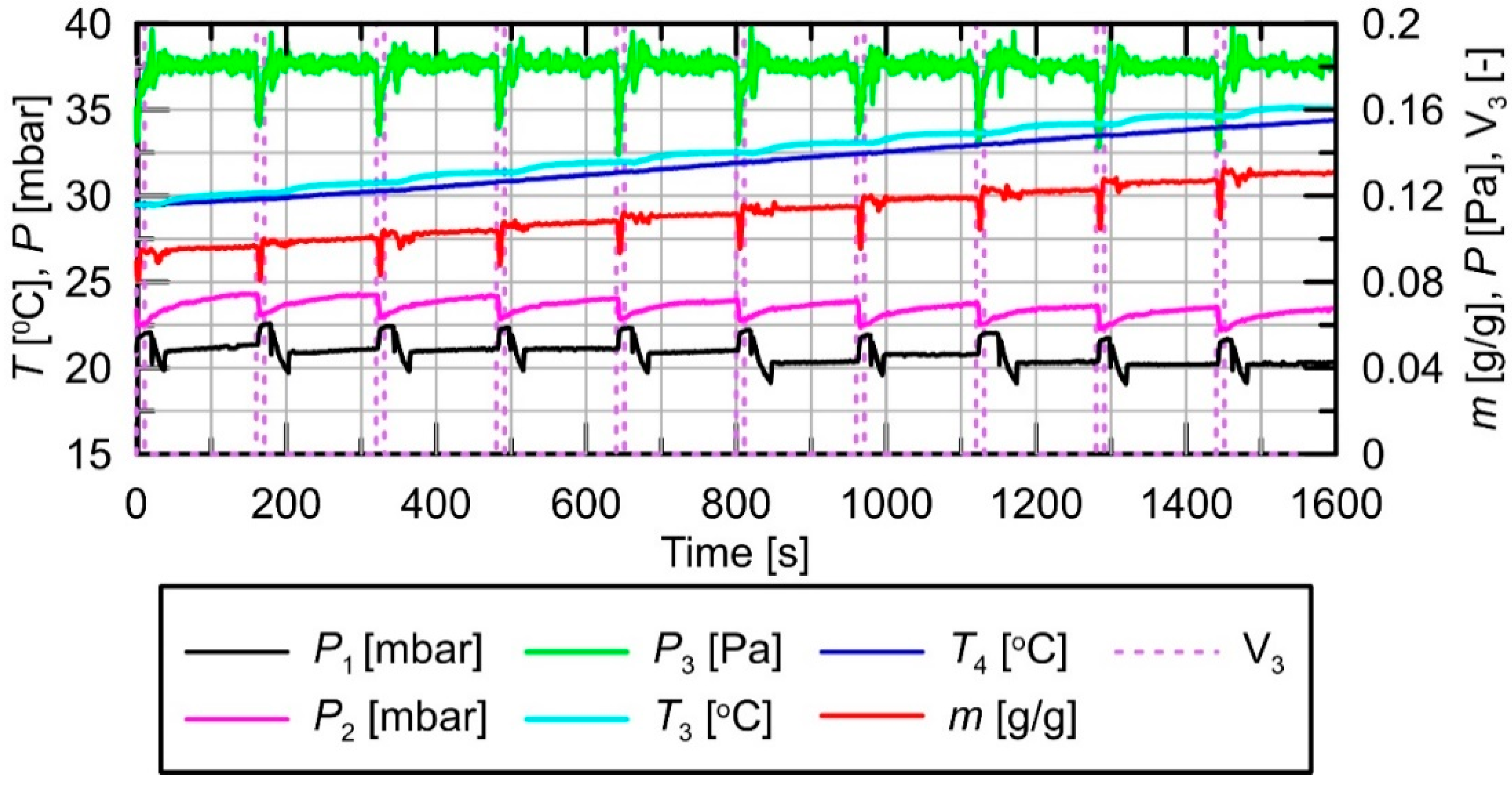
2.1. Experimental Test

The data needed to predict the adsorption bed’s mass comes from the previously conducted experimental studies carried out on the innovative test stand.
The test stand (Figure 2) consists of an evaporator, adsorption chamber, vacuum pump, three valves (V1, V2, V3), and sensors: P1—absolute pressure sensor in the adsorption chamber, P2—absolute pressure sensor in the evaporator, P3—relative pressure sensor, T1—temperature sensor in the adsorption chamber, T2—temperature sensor in the evaporator, T3—temperature sensor in the adsorption bed (bed center), T4—temperature sensor in the adsorption bed (25 mm from the bed center).
The first stage of work on the stand is to obtain the saturation pressure in the evaporator (P2) in the temperature T2. After obtaining the appropriate pressure for the evaporator (P2) and the chamber (P1), the water begins to boil, and the steam is released through the open valve (V3) to the sorption bed, where the adsorption process takes place. The changes taking place in the bed are monitored using temperature sensors T3, T4, and the relative pressure sensor P3 and mass sensors measuring the sorption bed’s weight. In the test process, assumptions were made for the valve opening/closing time (V3), according to Table 1. The table also shows the initial test conditions. Valves V1 and V2 are used to maintain the appropriate pressure difference in the evaporator and the adsorption chamber to keep the adsorbent’s fluidized and fixed beds.
Commercial silica gel from Fuji Silysia Chemical Ltd. (Greenville, USA) was employed for the research. Using the Analysette 3 Spartan shaker (FRITSCH GmbH, Idar-Oberstein, Germany), the material was separated to obtain granulation 250–300 µm. In the present study, aluminum (Al, granulation 45–450 µm) particles were used as an additive to improve the thermophysical properties of a silica gel (SG) adsorption bed, due to high thermal conductivity [51].
The exemplary results of the experiment are shown in Figure 3. They concern the tests of the 85% SG + 15%Al mixture for the stationary state. In this test and the other test variants (Table 1), the valve V3 was open for 10 s. The figure below shows ten consecutive opening and closing cycles of the valve V3.
Based on Table 1, experimental studies were performed, and the data from these experiments were used as inputs (P1, P2, P3, T3, T4, type of mixture, the percentage value of the additive) and outputs (sorption bed mass) of the LSTM network. Exemplary data that is entered into the LSTM network is shown in Figure 3; six such studies were performed as shown in Table 1. The test results from the six experiments were fed into the LSTM network as outlined above.

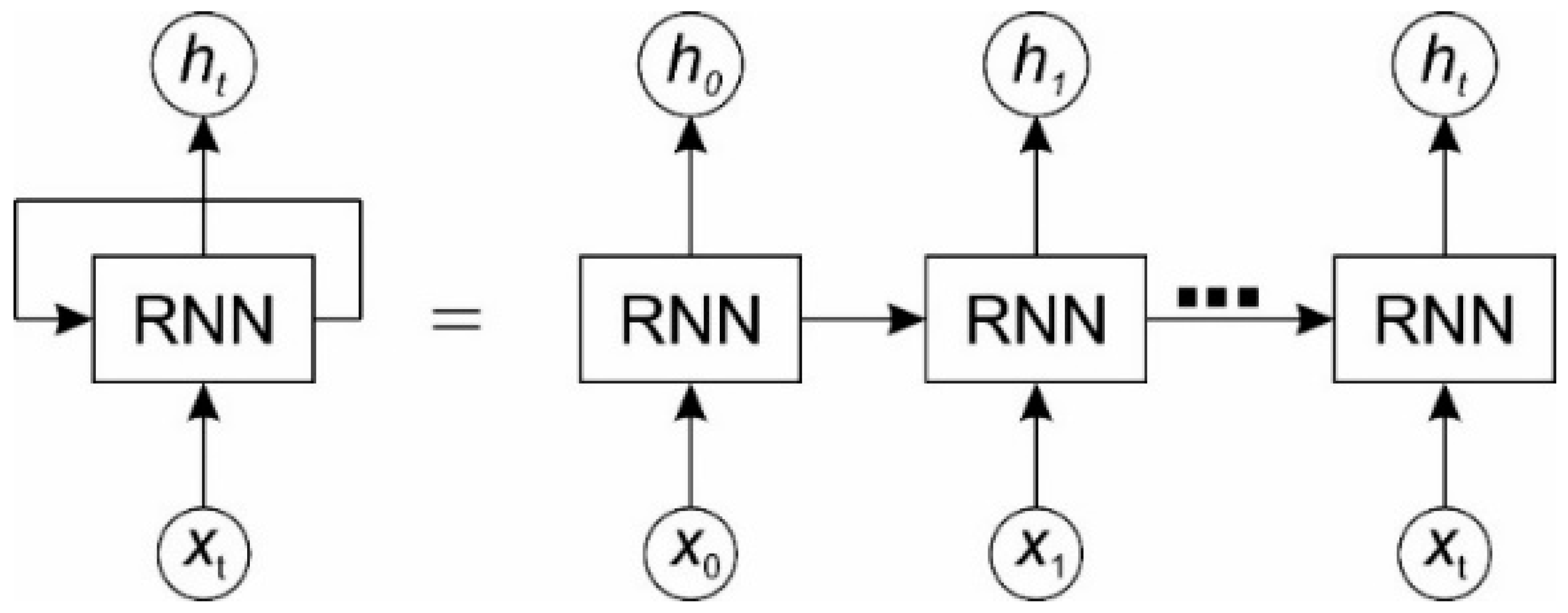
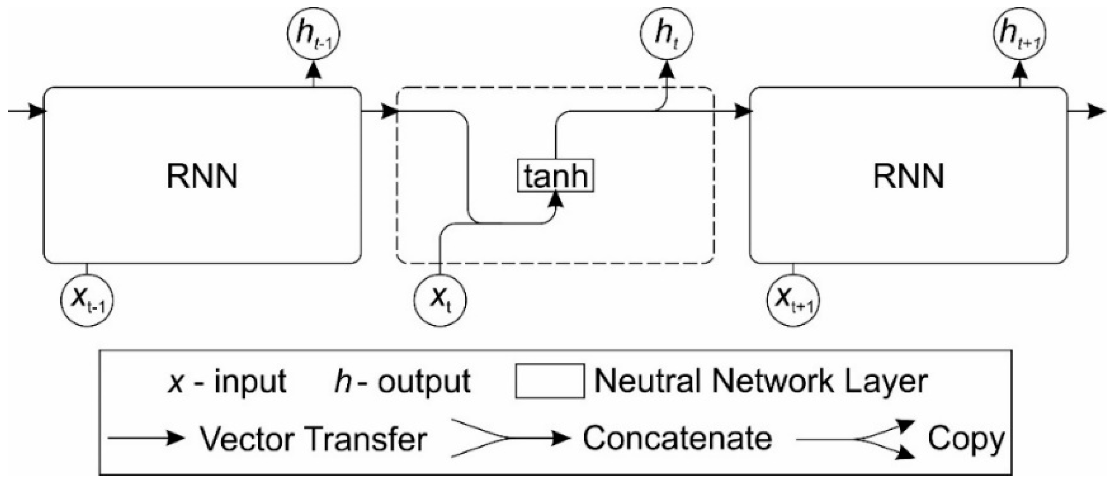
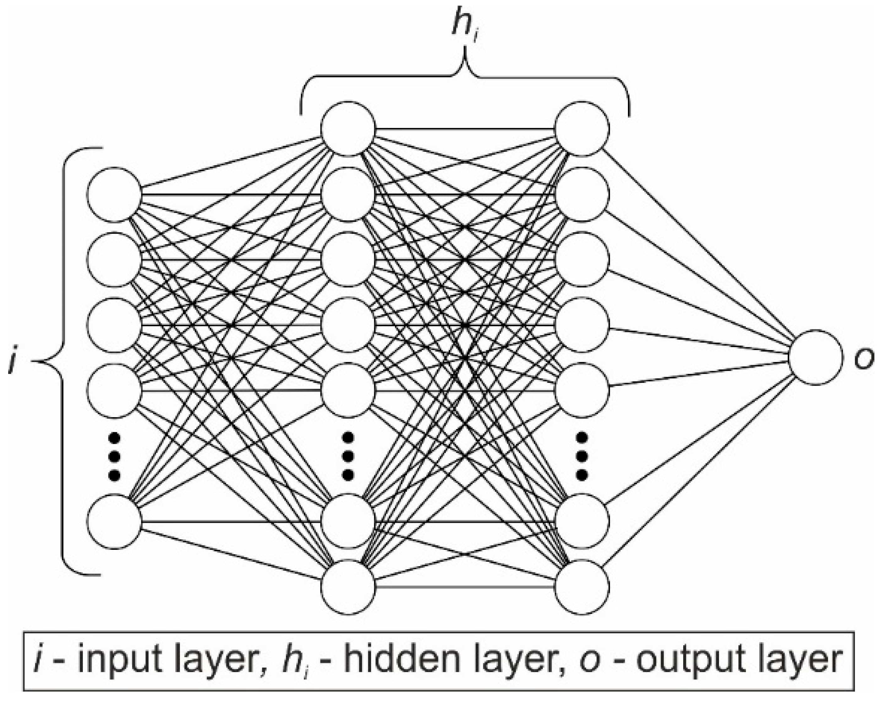
2.2. Recurrent Neural Network (RNN)

A recurrent Neural Network is a deep learning model consisting of neurons. It is mainly useful when considering sequence data, as each neuron can use its internal memory to store information about the previous input. This action resembles a loop (Figure 4) in which the output of a neuron at one specific stage is provided to the next neuron as an input. The RNN considers two inputs; the first is the current input, and the second is the previous computation [32]. RNNs contain an input layer, hidden layers, and; an output layer as with other neural networks.
All recurrent neural networks have the form of a chain of repeating modules of the neural network. In standard RNNs, this repeating module has a straightforward structure, such as a single tanh (hyperbolic tangent) layer (Figure 5).

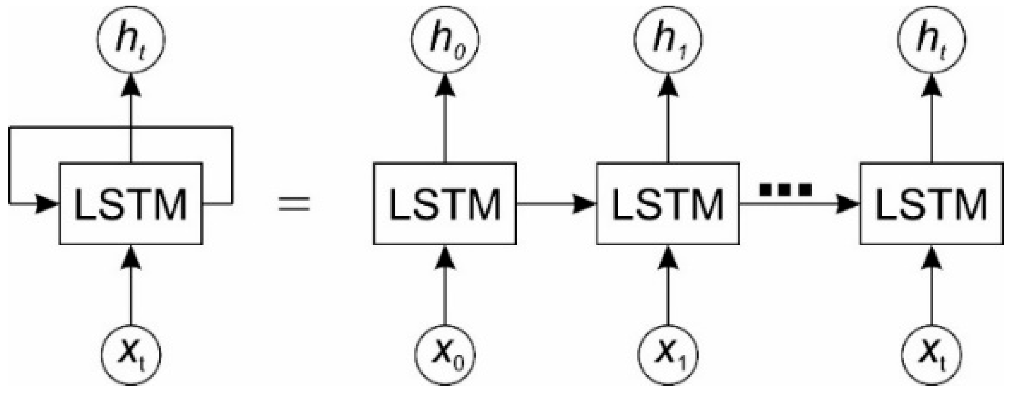
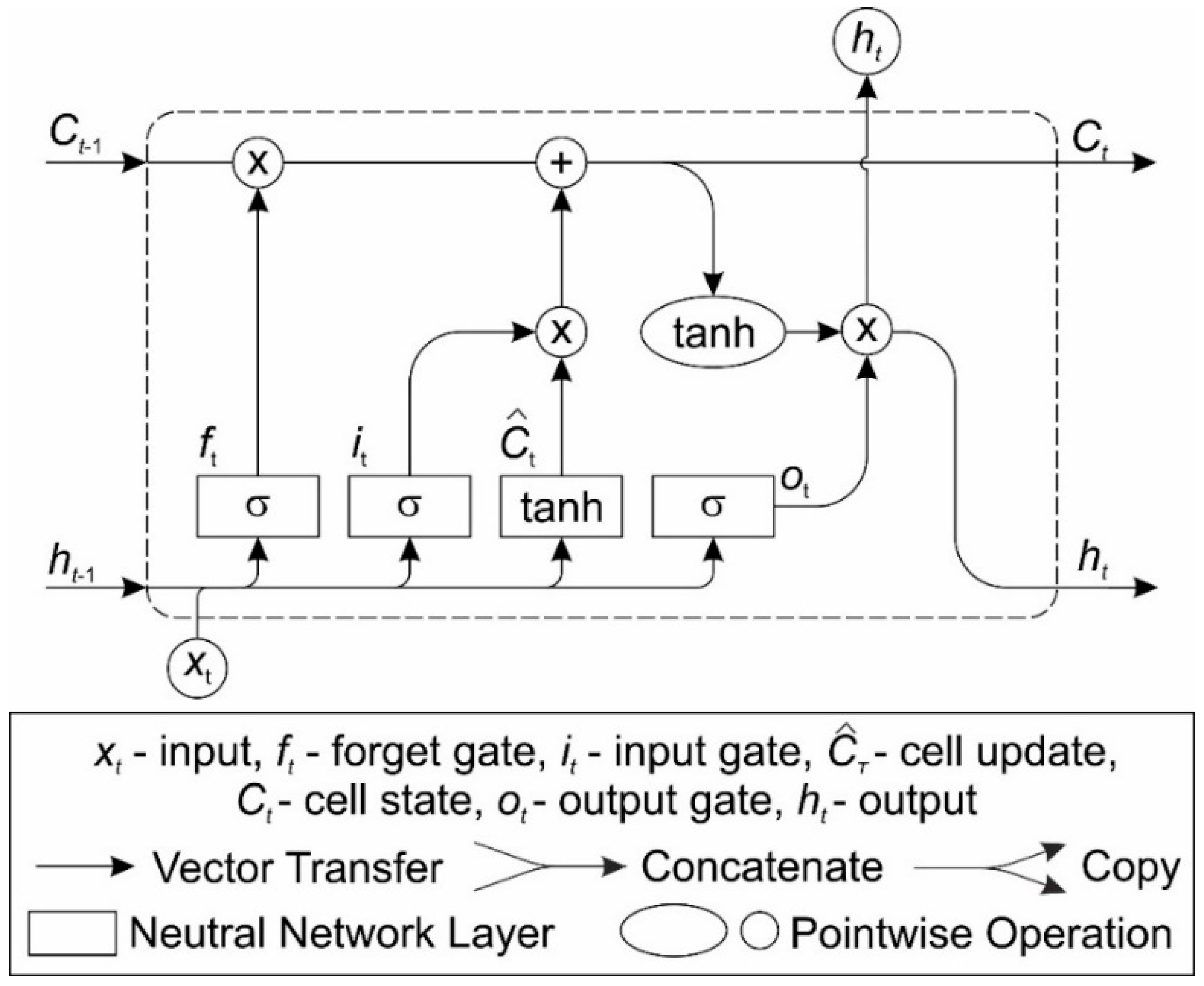
2.3. Long Short-Term Memory (LSTM)

Long Short-Term Memory networks (LSTMs) are a special kind of RNN, capable of learning long-term dependencies. They were introduced by Hochreiter and Schmidhuber in 1997 [17] and then refined and popularized by other researchers [52,53,54]. LSTMs have a chain-like structure show in Figure 6; the repeating module has a structure shown in Figure 7 (where tanh-hyperbolic tangent).
In order to implement the LSTM recurrent network, first, the LSTM cell should be implemented. The LSTM cell has three gates and two internal states, which should be determined to calculate the current output and current cell state. We distinguish the following LSTM cell gateways:
  • forget gate ft –filters information from the input and previous output and decides which information to remember or forget and discard,
  • input gate it –controls the flow of activation to enter the cell,
  • output gate ot –controls the output flow of cell activation.
In addition to these three gates, the LSTM cell contains a cell update usually activated by the tanh function.
Three variables fall into each LSTM cell:
  • input xt,
  • previous output ht−1
  • cell state Ct−1
Calculations for the LSTM cell in its individual layers can be described as follows.
  • the forget gate ft (sigmoid layer):
    f t = σ ( W f [ h t 1 , x t ] + b f )
  • the input gate it (sigmoid layer):
    i t = σ ( W i [ h t 1 , x t ] + b i )
  • the cell state Ct:
    c ^ t = tanh ( W c [ h t 1 , x t ] + b c )
    C t = f t · C t 1 + i t · c ^ t
  • the output gate ot (sigmoid layer):
    o t = σ ( W o [ h t 1 , x t ] + b o )
    where: c ^ t —the cell update; Wf, Wi, Wc, Wo—matrices of weights; bf, bi, bc, bo—bias vector.
The bias vector is specified as a numeric array. They are learnable parameters. When training the network, the biases vector in the first iteration is refilled with zeros.
The matrices of weights are specified as a numeric array, they are parameters that can be learned. The initial value of the weights in the algorithm is computed with the Glorot initializer [55] (also known as Xavier initializer). The Glorot initializer independently samples from a uniform distribution with zero mean and variance 2/(numIn + numOut) where numIn—number of inputs in i-th layer, numOut—number of outputs i-th layer.
The final stage of the calculations in the LSTM cell is defining the current output ht. The current output is calculated with the multiplication operation between the output gate layer and tanh layer of the current cell state Ct:
h t = o t · tanh ( C t )
The current output ht passes through the network as the previous state for the next LSTM cell or as the input for the neural network output layer.
The structure of the LSTM network is shown in Figure 8. The same network settings were adopted in all studies. Hyperparameters (Table 2) were selected on the basis of a series of studies not presented in this article. From the LSTM network tests carried out earlier, the hyperparameters’ values were selected based on the best fit. Every 30 epochs (the epoch is the full passage of the training algorithm through the entire training set) the learning coefficient changed its value according to the equation: ilr = 0.2 * lr (lr—current value of the learning coefficient).
The network input layer comprises the following inputs: P1—absolute pressure in the adsorption chamber, P2—absolute pressure in the evaporator, P3—relative pressure, T3—temperature in the adsorption bed (bed center), T4—the temperature in the adsorption bed (25 mm from the bed center), type of the mixture, and the percentage value of the addition. The mass of the sorption bed constitutes the output of the neural network.

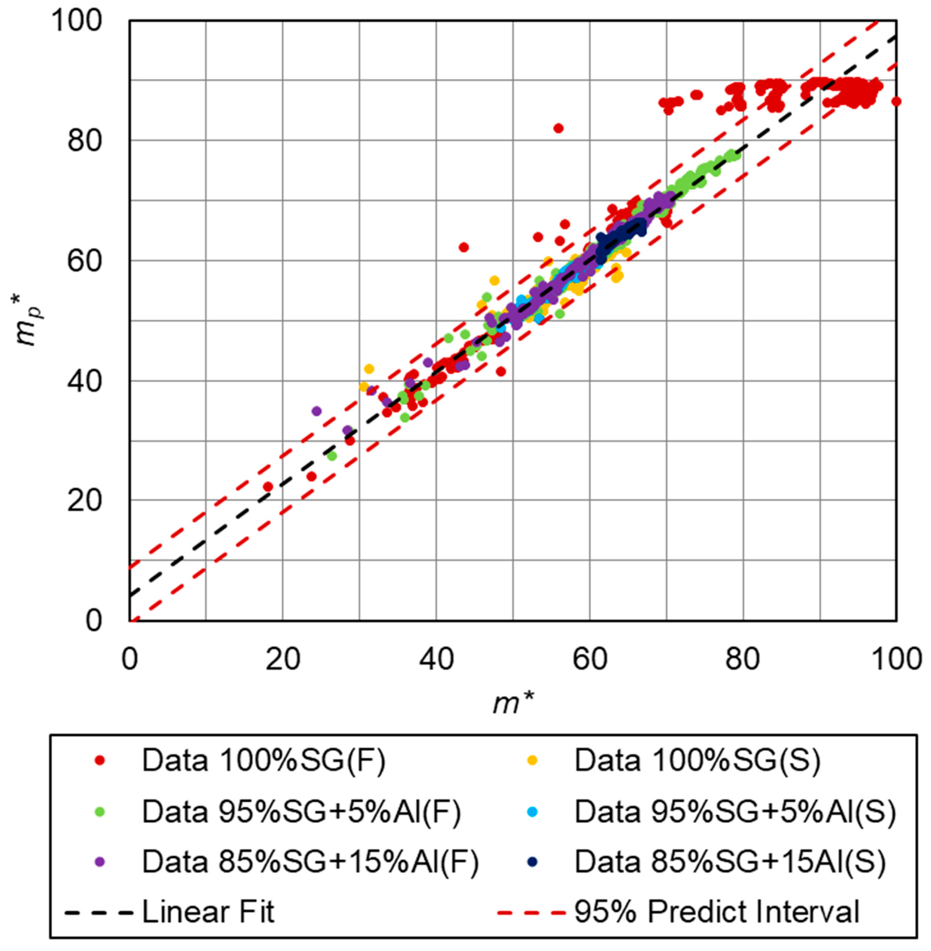
3. Results of Numerical Calculations

By adopting the assumptions, formulations, and experimental research results presented in the previous chapters, the LSTM network algorithm and a computer program were developed, which enabled predicting the sorption bed’s mass during the sorption process. The experimental test results for the first ten valve V3 opening cycles (6 tests, see Table 1) have been normalized to a range of 0 to 100 and divided into three parts. The training data is presented to the network during the training stage. Validation data is exploited to improve learning and possibly to stop training. Finally, the test data do not affect training and validation, and thus, provide an independent measurement of network performance after training. These data were randomized without duplication as follows:
(a)
First numerical research (60-20-20):
  • training data—60% of all data,
  • validation data—20% of all data,
  • test data—20% of all data,
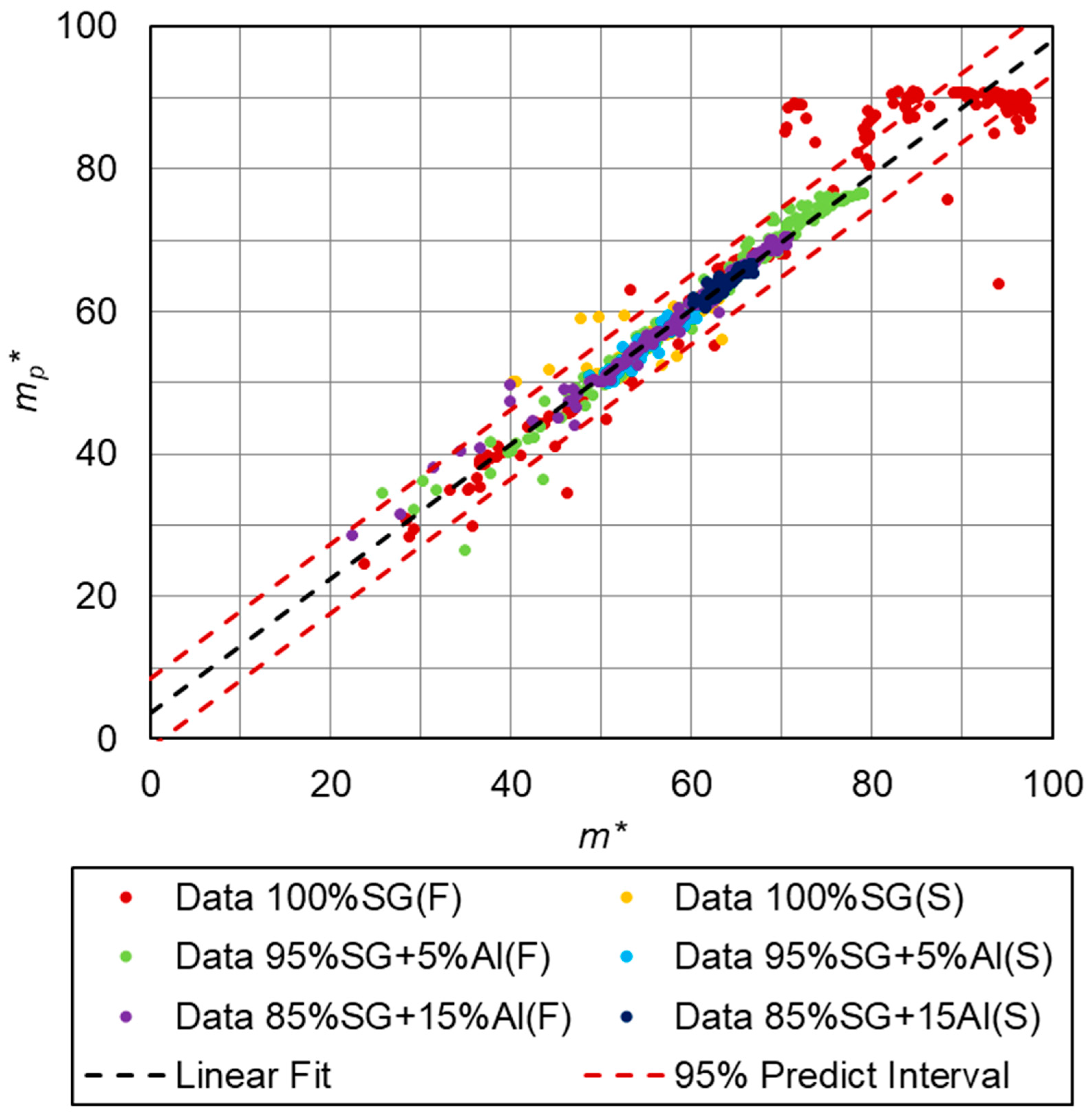
(b)
Second numerical research (70-15-15):
  • training data—70% of all data,
  • validation data—15% of all data,
  • test data—15% of all data,
(c)
Third numerical research (80-10-10):
  • training data—80% of all data,
  • validation data—10% of all data,
  • test data—10% of all data.
Figure 9, Figure 10 and Figure 11 show test data as the trend line (linear fit) for all studies and the 95% prediction interval of LSTM network results.
The first analysis of the prediction of mass in the sorption bed using the LSTM network concerned the division of data in the ratio of 60-20-20, the results of this study are shown in Figure 9 and Table 3.
Figure 9 shows the LSTM network operation results compared to the values obtained during the experiment. The LSTM network predicts the worst results for pure silica gel (100% SG) in a fluidized state.
Table 3 shows the fit for all data and individual mixture. The coefficient of determination for all data is 0.9515. The LSTM network predicts the worst values for pure silica gel (100% SG). In the case of fluidization, the coefficient of determination is 0.8934, and for the fixed bed, it is 0.9218, which may be the reason for the low repeatability of the cycles during the experiment. The network achieves the best match for the mixture 95% SG + 5%Al, where the coefficient of determination for fluidized and fixed bed was equal to 0.989, and 0.973, respectively.
The second analysis of mass prediction in the sorption bed using the LSTM network concerned the data division in the ratio of 70-15-15. The results of this study are presented in Figure 10 and Table 4.
Figure 10 shows the result of the LSTM network in comparison with the values obtained during the experiment. As in the previous study, the LSTM network predicts the worst results for pure silica gel (100% SG) in a fluidized state.
All datasets achieved a fit of 0.9507, and Table 4 also shows the coefficient of determination of the individual mixture for the fit function. The coefficient of determination in this study is lower than in the previous study. The LSTM network predicts the worst values for pure silica gel (100% SG) in fluidized bed conditions. The coefficient of determination for fixed and fluidized bed was 0.9250 and 0.8404, respectively.
The model’s best accuracy, in this case, was achieved for the fluidized bed of 85% SG + 15%Al mixture with R2 equal to 0.98.
The third analysis of the prediction of mass in the sorption bed using the LSTM network concerned the distribution of data in the ratio of 80-10-10. The results of this study are presented in Figure 11 and Table 5.
Figure 11 shows the results of the LSTM in comparison with the values obtained during the experiment. As in previous studies, the LSTM network predicts the worst results for pure silica gel (100% SG), fluidized state. In this case, the network best predicts the results of the experimental research.
The coefficient of determination for all is equal to 0.9554. The accuracy of the developed model is the best of the two previous ones. Only a slight decrease in R2 be seen for the 95% SG + 5%Al(S), and 95% SG + 15%Al(S) blends. The LSTM network prediction is still worst for the fluidized bed of pure silica gel (100% SG) with R2 equal to 0.867. However, the best prediction was achieved for the fluidized bed of the mixture 95% SG + 5%Al with R2 = 0.9915.

4. Conclusions

This paper deals with an innovative concept of a fluidized bed instead of a fixed adsorption beds application, currently employed in conventional adsorption chillers. The model, developed in the study, correctly predicts the vapor mass adsorbed in the adsorption chillers.
In this work, the Long Short-Term Memory networks, classified as a deep learning method, were also used to predict the sorption bed’s mass. The LSTM network is one of the particular kinds of recursive networks that are capable of learning long-term dependencies.
The solution to predicting the results was based on the most accurate mapping of the experimental values by the LSTM network. In the mathematical model, all network inputs were normalized to the range <0–100> due to the different units of parameters used in the study.
The analysis was performed by splitting the input data set into three parts (training data, validation data, and test data), in three variants: 60-20-20, 75-15-15, 80-20-20. The LSTM network, while increasing the amount of data used for training, better reproduced the experimental results. By increasing the training data make it possible to increase the accuracy of LSTM. The division of data into training data, validation data, and test data in deep learning networks are problematic because increasing one of the above values reduces the other two. A better solution seems to be to increase the amount of data entered into the network, but in this case, it was impossible due to the number of sorption cycles that the adopted mixtures could perform. In order to increase the amount of data, the mass of the mixture should be increased, as well as the initial conditions under which the tests were performed, e.g., the absolute pressure in the adsorption chamber and evaporator.
The developed model using the LSTM network and the high accuracy of the obtained numerical results confirm that the LSTM network is suitable for predicting sorption processes.
The LSTM network predicted the worst experimental test for pure silica gel (100% SG) in the fluidized conditions where the coefficient of determination did not exceed the threshold of 0.9 since these experimental tests are the least repeatable. The test results for 100% SG are more difficult to predict because no additive in the mixture would stabilize the sorption processes during the experimental test, so the sorption cycles for 100% SG are not very repeatable. Due to its high thermal conductivity, aluminum’s addition to the silica gel stabilizes the mixture, improving the sorption bed’s thermophysical properties. The LSTM network achieved the best accuracy for the mixture of 95% silica gel with 5% aluminum of addition in the fluidized conditions. For data splitting of 80-10-10 the highest coefficient of determination was equal to 0.9915.
Future research is planned to conduct comparative studies of several deep learning methods.

Author Contributions

The contribution of co-authors in creating article is: conceptualization, D.S., J.K.; methodology, D.S., J.K., software, D.S., J.K.; validation, D.S., J.K., M.S., W.N.; formal analysis, J.K., M.S.; investigation, A.K., A.Z., K.G., K.C.; resources, A.K., A.Z., K.G., D.S., K.C., M.S., J.K.; data curation, A.K., A.Z., K.G., D.S., M.S., J.K.; writing—original draft preparation, D.S., J.K.; writing—review and editing, D.S., M.S., J.K.; visualization, D.S., J.K., M.S.; supervision, J.K.; project administration, J.K., K.G.; funding acquisition, J.K., M.S., K.G. All authors have read and agreed to the published version of the manuscript.

Funding

This research was funded by project No. 2018/29/B/ST8/00442, supported by the National Science Centre.

Conflicts of Interest

The authors declare no conflict of interest.

Nomenclature

Alaluminum
Ffluidized state corresponding to fluidized bed conditions
LSTMLong Short-Term Memory
m*normalized sorbent mass (experimental value), –
mp*normalized sorbent mass predicted by the LSTM, –
NNneural network
n%the percentage of the additive in the mixture, %
RNNRecurrent Neural Network
Sstationary state corresponding to the fixed bed conditions
SGsilica gel

References

  1. Sosnowski, M. Evaluation of Heat Transfer performance of a Multi-Disc Sorption Bed Dedicated for Adsorption Cooling Technology. Energies 2019, 12, 4660. [Google Scholar] [CrossRef] [Green Version]
  2. Saha, B.B.; Koyama, S.; Lee, J.B.; Kuwahara, K.; Alam, K.C.A.; Hamamoto, Y.; Akisawa, A.; Kashiwagi, T. Performance evaluation of a low-temperature waste heat driven multi-bed adsorption chiller. Int. J. Multiph. Flow 2003, 29, 1249–1263. [Google Scholar] [CrossRef]
  3. Scapino, L.; Zondag, H.A.; Diriken, J.; Rindt, C.C.M.; Van Bael, J.; Sciacovelli, A. Modeling the performance of a sorption thermal energy storage reactor using artificial neural networks. Appl. Energy 2019, 253, 113525. [Google Scholar] [CrossRef]
  4. Argyropoulos, D.; Paraforos, D.S.; Alex, R.; Griepentrog, H.W.; Müller, J. NARX Neural Network Modelling of Mushroom Dynamic Vapour Sorption Kinetics. IFAC-PapersOnLine 2016, 49, 305–310. [Google Scholar] [CrossRef]
  5. Hua, J.; Faghri, A. Applications of artificial neural networks to intelligent vehicle-highway systems. Transp. Res. Rec. 1994, 1453, 83. [Google Scholar]
  6. Ashraf, W.M.; Uddin, G.M.; Arafat, S.M.; Afghan, S.; Kamal, A.H.; Asim, M.; Khan, M.H.; Rafique, M.W.; Naumann, U.; Niazi, S.G. Optimization of a 660 MWe Supercritical Power Plant Performance—A Case of Industry 4.0 in the Data-Driven Operational Management Part 1. Thermal Efficiency. Energies 2020, 13, 5592. [Google Scholar] [CrossRef]
  7. Ashraf, W.M.; Uddin, G.M.; Kamal, A.H.; Khan, M.H.; Khan, A.A.; Ahmad, H.A.; Ahmed, F.; Hafeez, N.; Sami, R.M.Z.; Arafat, S.M. Optimization of a 660 MWe Supercritical Power Plant Performance—A Case of Industry 4.0 in the Data-Driven Operational Management. Part 2. Power Generation. Energies 2020, 13, 5619. [Google Scholar] [CrossRef]
  8. Krzywanski, J.; Grabowska, K.; Herman, F.; Pyrka, P.; Sosnowski, M.; Prauzner, T.; Nowak, W. Optimization of a three-bed adsorption chiller by genetic algorithms and neural networks. Energy Convers. Manag. 2017, 153, 313–322. [Google Scholar] [CrossRef]
  9. Krzywanski, J. A General Approach in Optimization of Heat Exchangers by Bio-Inspired Artificial Intelligence Methods. Energies 2019, 12, 4441. [Google Scholar] [CrossRef] [Green Version]
  10. Krzywanski, J.; Grabowska, K.; Sosnowski, M.; Zylka, A.; Sztekler, K.; Kalawa, W.; Wojcik, T.; Nowak, W. An adaptive neuro-fuzzy model of a re-heat two-stage adsorption chiller. Therm. Sci. 2019, 23, 1053–1063. [Google Scholar] [CrossRef] [Green Version]
  11. Park, D.; Rilett, L.R. Forecasting freeway link travel times with a multilayer feed-forward neural network. Comput. Aided Civ. Infrastruct. Eng. 1999, 14, 357–367. [Google Scholar] [CrossRef]
  12. Yin, H.; Wong, S.; Xu, J.; Wong, C. Urban traffic flow prediction using a fuzzy-neural approach. Transp. Res. Part C Emerg. Technol. 2002, 10, 85–98. [Google Scholar] [CrossRef]
  13. Van Lint, J.; Hoogendoorn, S.; Van Zuylen, H. Freeway travel time prediction with state-space neural networks: Modeling state-space dynamics with recurrent neural networks. Transp. Res. Rec. J. Transp. Res. Board 2002, 1811, 30–39. [Google Scholar] [CrossRef]
  14. Yu, R.; Li, Y.; Shahabi, C.; Demiryurek, U.; Liu, Y. Deep learning: A generic approach for extreme condition traffic forecasting. In Proceedings of the 2017 SIAM International Conference on Data Mining, Houston, TX, USA, 27–29 April 2017; pp. 777–785. [Google Scholar]
  15. Jozefowicz, R.; Zaremba, W.; Sutskever, I. An empirical exploration of recurrent network architectures. In Proceedings of the 32nd International Conference on Machine Learning (ICML-15), Lille, France, 6–11 July 2015; pp. 2342–2350. [Google Scholar]
  16. Liu, H.; Chen, C. Data processing strategies in wind energy forecasting models and applications: A comprehensive review. Appl. Energy 2019, 249, 392–408. [Google Scholar] [CrossRef]
  17. Hochreiter, S.; Schmidhuber, J. Long short-term memory. Neural Comput. 1997, 9, 1735–1780. [Google Scholar] [CrossRef]
  18. Vinyals, O.; Toshev, A.; Bengio, S.; Erhan, D. Show and tell: A neural image caption generator. In Proceedings of the IEEE Conference on Computer Vision and Pattern Recognition, Boston, MA, USA, 7–12 June 2015; pp. 3156–3164. [Google Scholar]
  19. Eck, D.; Schmidhuber, J. A first look at music composition using lstm recurrent neural networks. Istituto Dalle Molle Di Studi Sull Intelligenza Artificiale 2002, 103, 48. [Google Scholar]
  20. Shahid, F.; Zameer, A.; Muneeb, M. Prediction for COVID-19 with deep learning models of LSTM, GRU, and Bi-LSTM. Choas Solitions Fractals 2020, 140, 110212. [Google Scholar] [CrossRef]
  21. Graves, A.; Mohamed, A.-R.; Hinton, G. Speech recognition with deep recurrent neural networks. In Proceedings of the 2013 IEEE International Conference on Acoustics, Speech and Signal Processing, Vancouver, BC, Canada, 26–31 May 2013; pp. 6645–6649. [Google Scholar] [CrossRef] [Green Version]
  22. Alahi, A.; Goel, K.; Ramanathan, V.; Robicquet, A.; Fei-Fei, L.; Savarese, S. Social lstm: Human trajectory prediction in crowded spaces. In Proceedings of the IEEE Conference on Computer Vision and Pattern Recognition, Las Vegas, NV, USA, 26 June–1 July 2016; pp. 961–971. [Google Scholar]
  23. Martinez-Garcia, M.; Zhang, Y.; Suzuki, K.; Zhand, Y.-D. Deep Recurrent Entropy Adaptive Model for System Reliability Monitoring. IEEE Trans. Ind. Inform. 2020, 17, 839–848. [Google Scholar] [CrossRef]
  24. Martinez-Garcia, M.; Zhang, Y.; Gordon, T. Memory pattern identification for feedback tracking control in human-machine system. Hum. Factors 2019. [Google Scholar] [CrossRef] [Green Version]
  25. Chen, Y.-Y.; Lv, Y.; Li, Z.; Wang, F.-Y. Long short-term memory model for traffic congestion prediction with online open data. In Proceedings of the 2016 IEEE 19th International Conference on Intelligent Transportation Systems (ITSC), Rio de Janeiro, Brazil, 1–4 November 2016; pp. 132–137. [Google Scholar] [CrossRef]
  26. Wu, Y.; Tan, H. Short-term traffic flow forecasting with spatial temporal correlation in a hybrid deep learning framework. arXiv 2016, arXiv:1612.01022. [Google Scholar]
  27. Ma, X.; Tao, Z.; Wang, Y.; Yu, H.; Wang, Y. Long short-term memory neural network for traffic speed prediction using remote microwave sensor data. Transp. Res. Part C Emerg. Technol. 2015, 54, 187–197. [Google Scholar] [CrossRef]
  28. Duan, Y.; Lv, Y.; Wang, F.-Y. Travel time prediction with lstm neural network. In Proceedings of the 2016 IEEE 19th International Conference on Intelligent Transportation Systems (ITSC), Rio de Janeiro, Brazil, 1–4 November 2016; pp. 1053–1058. [Google Scholar] [CrossRef]
  29. Fu, R.; Zhang, Z.; Li, L. Using lstm and gru neural network methods for traffic flow prediction. In Proceedings of the 2016 31st Youth Academic Annual Conference of Chinese Association of Automation (YAC), Wuhan, China, 11–13 November 2016; pp. 324–328. [Google Scholar] [CrossRef]
  30. Zhao, Z.; Chen, W.; Wu, X.; Chen, P.C.; Liu, J. Lstm network: A deep learning approach for short-term traffic forecast. IET Intell Transp. Syst. 2017, 11, 68–75. [Google Scholar] [CrossRef] [Green Version]
  31. Graves, A.; Jaitly, N.; Mohamed, A.-R. Hybrid speech recognition with deep bidirectional LSTM. In Proceedings of the 2013 IEEE Workshop on Automatic Speech Recognition and Understanding, Olomouc, Czech Republic, 8–12 December 2013; pp. 273–278. [Google Scholar] [CrossRef]
  32. LeCun, Y.; Bengio, Y.; Hinton, G. Deep learning. Nature 2015, 521, 436–444. [Google Scholar] [CrossRef] [PubMed]
  33. Lipton, Z.C.; Berkowitz, J.; Elkan, C. A critical review of recurrent neural networks for sequence learning. arXiv 2015, arXiv:1506.00019. [Google Scholar]
  34. Kirbas, I.; Sozen, A.; Tuncer, A.D.; Kazancioglu, F.S. Comparative analysis and forecasting of Covid-19 cases in various European countries with ARIMA, NARN and LSM approaches. Chaos Solitons Fractals 2020, 138. [Google Scholar] [CrossRef]
  35. Chitra, M.; Sutha, S.; Pappa, N. Application of deep neural techniques in predictive modelling for the estimation of Escherichia coli growth rate. J. Appl. Microbiol. 2020. [Google Scholar] [CrossRef]
  36. Thapa, S.; Zhao, Z.; Li, B.; Lu, L.; Fu, D.; Shi, X.; Tang, B.; Qi, H. Snowmelt-Driven Streamflow Prediction Using Machine Learning Techniques (LSTM, NARX, GPR, and SVR). Water 2020, 12, 1734. [Google Scholar] [CrossRef]
  37. Box, G.E.; Jenkins, G.M.; Reinsel, G.C.; Ljung, G.M. Time Series Analysis: Forecasting and Control; John Wiley & Sons: Hoboken, NJ, USA, 2015. [Google Scholar]
  38. Krzywanski, J.; Grabowska, K.; Sosnowski, M.; Zylka, A.; Kulakowska, A.; Czakiert, T.; Sztekler, K.; Wesolowska, M.; Nowak, W. Heat transfer in fluidized and fixed beds of adsorption chillers. E3S Web Conf. 2019, 128, 01003. [Google Scholar] [CrossRef]
  39. Krzywanski, J.; Grabowska, K.; Sosnowski, M.; Zylka, A.; Kulakowska, A.; Czakiert, T.; Wesolowska, M.; Nowak, W. Heat transfer in adsorption chillers with fluidized beds of silica gel, zeolite, and carbon nanotubes. Heat Transf. Eng. 2019, 128, 01003. [Google Scholar]
  40. Stanek, W.; Gazda, W.; Kostowski, W. Thermo-ecological assessment of CCHP (combined cold-heat-and-power) plant supported with renewable energy. Energy 2015, 92, 279–289. [Google Scholar] [CrossRef]
  41. Stanek, W.; Gazda, W. Exergo-ecological evaluation of adsorption chiller system. Energy 2014, 76, 42–48. [Google Scholar] [CrossRef]
  42. Aristov, Y.I. Review of adsorptive heat conversion/storage in cold climate countries. Appl. Therm. Eng. 2020, 180, 115848. [Google Scholar] [CrossRef]
  43. Krzywanski, J.; Żyłka, A.; Czakiert, T.; Kulicki, K.; Jankowska, S.; Nowak, W. A 1.5D model of a complex geometry laboratory scale fuidized bed clc equipment. Powder Technol. 2017, 316, 592–598. [Google Scholar] [CrossRef]
  44. Muskała, W.; Krzywański, J.; Czakiert, T.; Nowak, W. The research of CFB boiler operation for oxygen-enhanced dried lignite combustion. Rynek Energii 2011, 1, 172–176. [Google Scholar]
  45. Krzywanski, J.; Fan, H.; Feng, Y.; Shaikh, A.R.; Fang, M.; Wang, Q. Genetic algorithms and neural networks in optimization of sorbent enhanced H2 production in FB and CFB gasifiers. Energy Convers. Manag. 2018, 171, 1651–1661. [Google Scholar] [CrossRef]
  46. Chorowski, M.; Pyrka, P. Modelling and experimental investigation of an adsorption chiller using low-temperature heat from cogeneration. Energy 2015, 92, 221–229. [Google Scholar] [CrossRef]
  47. Rogala, Z.; Kolasiński, P.; Gnutek, Z. Modelling and experimental analyzes on air-fluidised silica gel-water adsorption and desorption. Appl. Therm. Eng. 2017, 127, 950–962. [Google Scholar] [CrossRef]
  48. Aristov, Y.I.; Glaznev, I.S.; Girnik, I.S. Optimization of adsorption dynamics in adsorptive chillers: Loose grains configuration. Energy 2012, 46, 484–492. [Google Scholar] [CrossRef]
  49. Girnik, I.S.; Grekova, A.D.; Gordeeva, L.G.; Aristov, Y.I. Dynamic optimization of adsorptive chillers: Compact layer vs. bed of loose grains. Appl. Therm. Eng. 2017, 125, 823–829. [Google Scholar] [CrossRef]
  50. Grabowska, K.; Krzywanski, J.; Nowak, W.; Wesolowska, M. Construction of an innovative adsorbent bed configuration in the adsorption chiller - Selection criteria for effective sorbent-glue pair. Energy 2018, 151, 317–323. [Google Scholar] [CrossRef]
  51. Grabowska, K.; Sztekler, K.; Krzywanski, J.; Sosnowski, M.; Stefanski, S.; Nowak, W. Construction of an innovative adsorbent bed configuration in the adsorption chiller part 2. experimental research of coated bed samples. Energy 2021, 215, 119123. [Google Scholar] [CrossRef]
  52. Kulakowska, A.; Pajdak, A.; Krzywanski, J.; Grabowska, K.; Zylka, A.; Sosnowski, M.; Wesolowska, M.; Sztekler, K.; Nowak, W. Effect of Metal and Carbon Nanotube Additives on the Thermal Diffusivity of a Silica Gel-Based Adsorption Bed. Energies 2020, 13, 1391. [Google Scholar] [CrossRef] [Green Version]
  53. Song, X.; Kanasugi, H.; Shibasaki, R. Deep transport: Prediction and simulation of human mobility and transportation mode at a citywide level. In Proceedings of the Twenty-Fifth International Joint Conference on Artificial Intelligence, New York, NY, USA, 9–15 July 2016; pp. 2618–2624. [Google Scholar]
  54. Yu, H.; Wu, Z.; Wang, S.; Wang, Y.; Ma, X. Spatiotemporal Recurrent Convolutional Networks for Traffic Prediction in Transportation Networks. arXiv 2017, arXiv:1705.02699, 1501. [Google Scholar] [CrossRef] [PubMed] [Green Version]
  55. Glorot, X.; Youshua, B. Understanding the difficult of training deep feedforward neural networks. In Proceedings of the Thirteen International Conference on Artificial Intelligence and Statistics, Sardinia, Italy, 13–15 May 2010; pp. 249–256. [Google Scholar]
Figure 1. Scheme of adsorption chiller.
Energies 13 06601 g001
Figure 2. The testing stand and diagram of the test stand.
Energies 13 06601 g002
Figure 3. An exemplary result of the experimental test for the mixture 85%SG + 15%Al stationary state for ten consecutive cycles of valve V3 opening and closing.
Energies 13 06601 g003
Figure 4. An unrolled Recurrent Neural Network.
Energies 13 06601 g004
Figure 5. The repeating module in a standard RNN contains a single layer.
Energies 13 06601 g005
Figure 6. An unrolled LSTM.
Energies 13 06601 g006
Figure 7. Graphical representation of the LSTM cell.
Energies 13 06601 g007
Figure 8. Diagram of the LSTM network.
Energies 13 06601 g008
Figure 9. Comparison of the experimental results with the numerical results predicted by the LSTM (60-20-20).
Energies 13 06601 g009
Figure 10. Comparison of the experimental results with the numerical results predicted by the LSTM (70-15-15).
Energies 13 06601 g010
Figure 11. Comparison of the experimental results with the numerical results predicted by the LSTM (80-10-10).
Energies 13 06601 g011
Table 1. Initial research conditions.
No.Type of MaterialAdditive to the Mixturet0 [s] 1tz [s] 2P1 [bar] 3P2 [bar] 4StateMass of Sorbent in the Bed [g]
1100%SG 5-101501323F 755
2100%SG 5-101502123S 855
395%SG 5+5%Al 6101501323F 755
495%SG 5+5%Al 6101502123S 855
585%SG 5+15%Al 6101501323F 755
685%SG 5+15%Al 6101502123S 855
1 the opening time of valve V3, 2 stabilizing time of conditions in the chamber (valve V3 state—closed), 3 pressure in the chamber, 4 pressure in the evaporator, 5 silica gel, 6 aluminum, 7 fluidized state, 8 stationary state.
Table 2. The values of the hyperparameters for the LSTM.
HyperparameterValue
Number of epochs200
Learning rate0.005
Number of LSTM layers2
Number of cells in layer 1210
Number of cells in layer 2190
Drop out layer0.05
Table 3. Coefficient of determination R2 for the Linear Fit (60-20-20).
R2
All Data100%SG (F)100%SG (S)95%SG +5%Al (F)95%SG +5%Al (S)85%SG +15%Al (F)85%SG +15%Al (S)
0.95150.89340.92180.98910.97320.98480.9505
Table 4. Coefficient of determination R2 for the Linear Fit (70-15-15).
R2
All Data100%SG (F)100%SG (S)95%SG +5%Al (F)95%SG +5%Al (S)85%SG +15%Al (F)85%SG +15%Al (S)
0.95070.84040.92500.97880.97380.98000.9363
Table 5. Coefficient of determination R2 for the Linear Fit (80-10-10).
R2
All Data100%SG (F)100%SG (S)95%SG +5%Al (F)95%SG +5%Al (S)85%SG +15%Al (F)85%SG +15%Al (S)
0.95540.86700.93430.99150.96110.98740.9244
Publisher’s Note: MDPI stays neutral with regard to jurisdictional claims in published maps and institutional affiliations.

