Wind Farm Fault Detection by Monitoring Wind Speed in the Wake Region

Abstract

A novel concept of wind farm fault detection by monitoring the wind speed in the wake region is proposed in this study. A wind energy dissipation model was coupled with a computational fluid dynamics solver to simulate the fluid field of a wind turbine array, and the wind velocity and direction in the simulation were exported for identifying wind turbine faults. The 3D steady Navier–Stokes equations were solved by using the cell center finite volume method with a second order upwind scheme and a $k-\epsilon$ turbulence model. In addition, the wind energy dissipation model, derived from energy balance and Betz’s law, was added to the Navier–Stokes equations’ source term. The simulation results indicate that the wind speed distribution in the wake region contains significant information regarding multiple wind turbine faults. A feature selection algorithm specifically designed for the analysis of wind flow was proposed to reduce the number of features. This algorithm proved to have better performance than fuzzy entropy measures and recursive feature elimination methods under a limited number of features. As a result, faults in the wind turbine array could be detected and identified by machine learning algorithms.

1. Introduction

Wind energy is one of the renewable and non-polluting energy sources. It has become widely popular and is expected to replace conventional energy sources, such as nuclear energy and coal. Wind turbines are used to convert wind energy into electricity. As higher wind speeds can be achieved offshore compared to on land, offshore wind farms with a large number of wind turbines can harvest higher wind energy to generate electricity. The offshore wind farms also have the advantages of not affecting the landscape and the ecological environment [1]. However, offshore wind farms are difficult to reach and have high maintenance costs due to the faults in the wind turbines. Therefore, condition monitoring systems and fault detection systems are required to identify and diagnose wind turbine faults to achieve satisfactory performance and avoid catastrophic disasters. Till date, numerous studies have measured different sensor signals such as vibration [2,3], current [4], acoustic emission (AE) [5], torque [6], and temperature [7] to detect faults in wind turbines. The general scheme of wind turbine fault detection is illustrated in Figure 1 [8,9]. These approaches based on signal processing require the installation of sensors in each wind turbine, thus increasing the cost of condition monitoring systems for offshore wind farms.

Research in condition monitoring and fault diagnosis of offshore wind turbines has a significant role in reducing the operation and maintenance costs. In fact, wind turbine faults are caused by failures of key components in the system, such as main bearings, gearboxes, and generators [10]. Vibration signal analysis is one of the most common approaches to gearbox monitoring and diagnostics. Signal processing approaches, such as fast Fourier transform, wavelet transform, and short-time Fourier transform, are often applied to analyze the vibration signal. The frequency content of the signal shows instructive information for bearing and gearbox monitoring. The relationship between the vibration signals and the evolution of front bearing faults has been shown on the frequency spectrum, in which the amplitude of a characteristic frequency is proportional to the bearing wear. Vibration analysis in the frequency domain is more advantageous in this case [11]. Igba et al. used features of vibration signals for condition monitoring of wind turbine gearboxes, in which the root mean square (RMS) and peak values proved to be good indicators of the gearbox health [12]. Vibration signal analysis, however, could increase the cost of wind farms because it requires the installation of vibration sensors on each turbine. Current-based monitoring techniques have been used to identify faults in wind turbines, and have proved to be effective in detecting gearbox faults [13]. Cheng et al. used experimental stator and rotor current signals and analyzed them in the frequency domain. It was found that the amplitudes of the characteristic frequency components were closely related to the wind turbine gearbox health. Wind turbine gearbox faults could be detected by monitoring the amplitudes of the fault characteristic frequencies [14]. However, the incapability of locating the faults is one of the main limitations of using motor current signal analysis [15]. Recently, AE signals have been considered as an effective technique for monitoring bearing and gearboxes of wind turbines, especially for early detection of cracking and pitting with extremely slow bearing rotational speeds [16,17]. AE sensing is a suitable enhancement to the classic vibration-based methods and can identify and distinguish the type of fault that occurs and provide precise diagnostics [18]. However, owing to the noisy background produced by the disturbance of wind and other rotational components of the wind turbine, the accuracy of fault detection could be reduced. This is the most challenging issue when using AE sensors for monitoring turbine faults.

The wind in the wake region behind offshore wind turbines has the characteristics of velocity deficit, low-frequency meandering, intermittent edge, and shear-layer-generated turbulence. At different distances behind the wind turbine, the dimensionless wake velocity deficit profiles reach minimum values around the center, and the wake velocity deficit is axisymmetric with respect to the hub [19]. Robert Menke et al. investigated wind turbine wake flow on complex terrain using six scanning wind light detection and ranging (Lidar) systems. The horizontal wind speed was measured and it showed that the deficit with a local minimum in the wake center was obtained at around 1D distance (D refers to the wind turbine diameter). The maximum deficit was decreased with the increase of distance behind the wind turbine [20]. The lowest velocity in the wake region could be achieved at around 2D downstream of the hub, and the distance between 2D and 5D was considered as the end of the near wake region [21,22]. Tamol conducted studies on the wake of a horizontal-axis wind turbine model and showed that the maximum velocity loss points tend to move below the rotor axis and lead to a non-symmetric distribution of atmospheric turbulence [23].

Most of the wind farm simulation studies have selected the linearized wake model, the actuator disk model, or direct simulation. Nowadays, the linearized wake model is often used in engineering practice, especially for the optimal design of wind farm layouts [24]. The linearized wake model assumes that wake is expanded linearly as a function of downstream distance. However, the area affected by wind turbine wake is nonlinearly outward [25]. Additionally, the actuator disk model uses a pressure jump to simulate the wind flow passing through the wind turbine [26]. The pressure jump is a function of the rotor disk area and the thrust force of the turbine. However, the turbine thrust force is almost unknown. Furthermore, a large number of computing resources are required for the direct simulation. This study uses the wind energy dissipation model, which is very similar to the porous media model, but only adopts the inertial loss term to simulate the wind energy losses in the wind turbine rotor.

In this study, the wind speeds at different distances in the wake region behind the wind turbine array were used to generate several statistical features relevant to the performance of offshore wind turbines. A novel feature selection algorithm based on the distance between feature distributions was proposed specifically for extracting significant information from the wind speed in the wake region and improving the classification accuracy. Machine learning methods such as artificial neural network (ANN), k-nearest neighbors (KNN), support vector machine (SVM), and similarity classifier (SC) were then applied to identify wind turbine status. Those machine learning techniques are advantageous for condition monitoring because of their ability to represent complex and nonlinear relationships such as wind speed in the wake region through a learned pattern recognition.

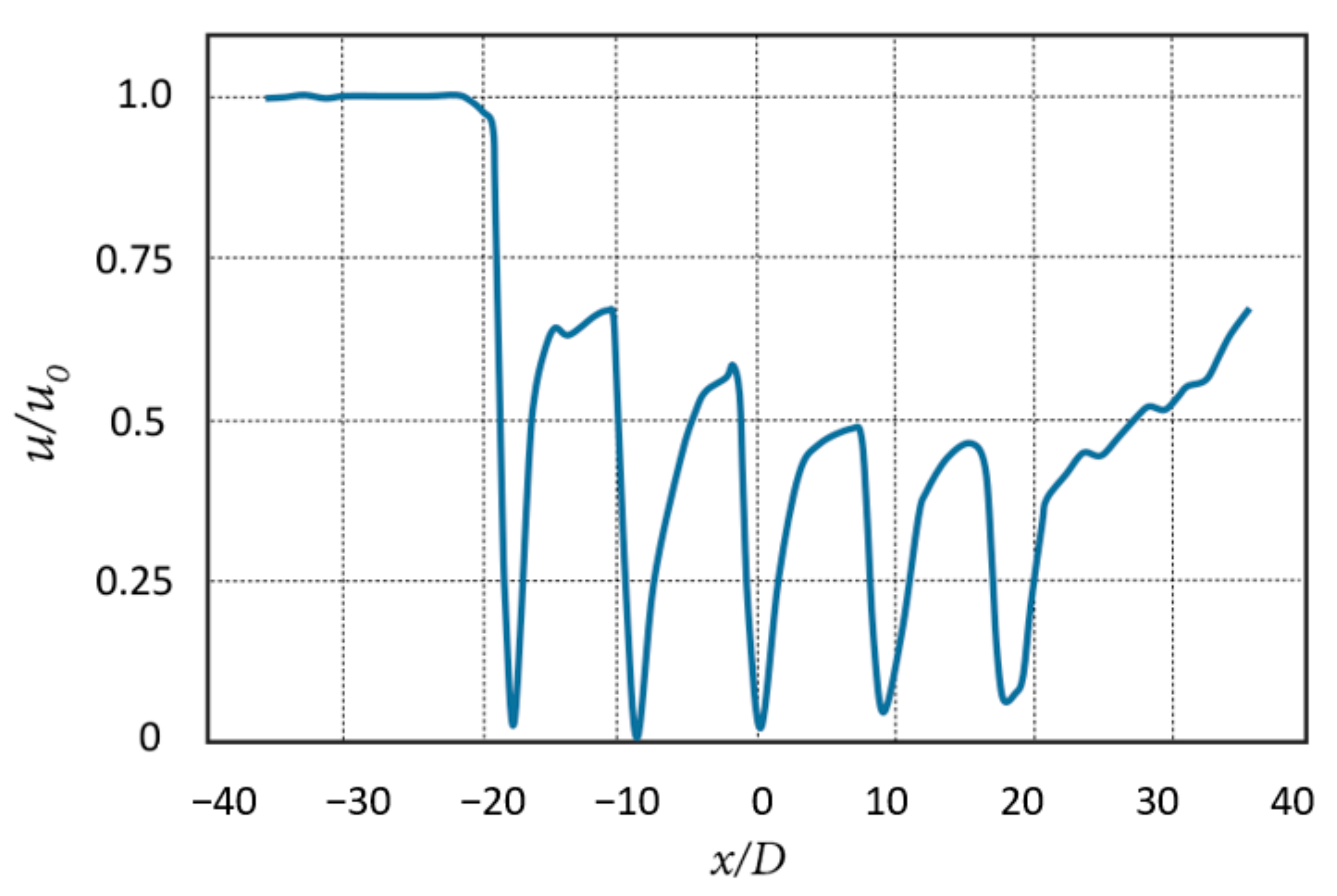
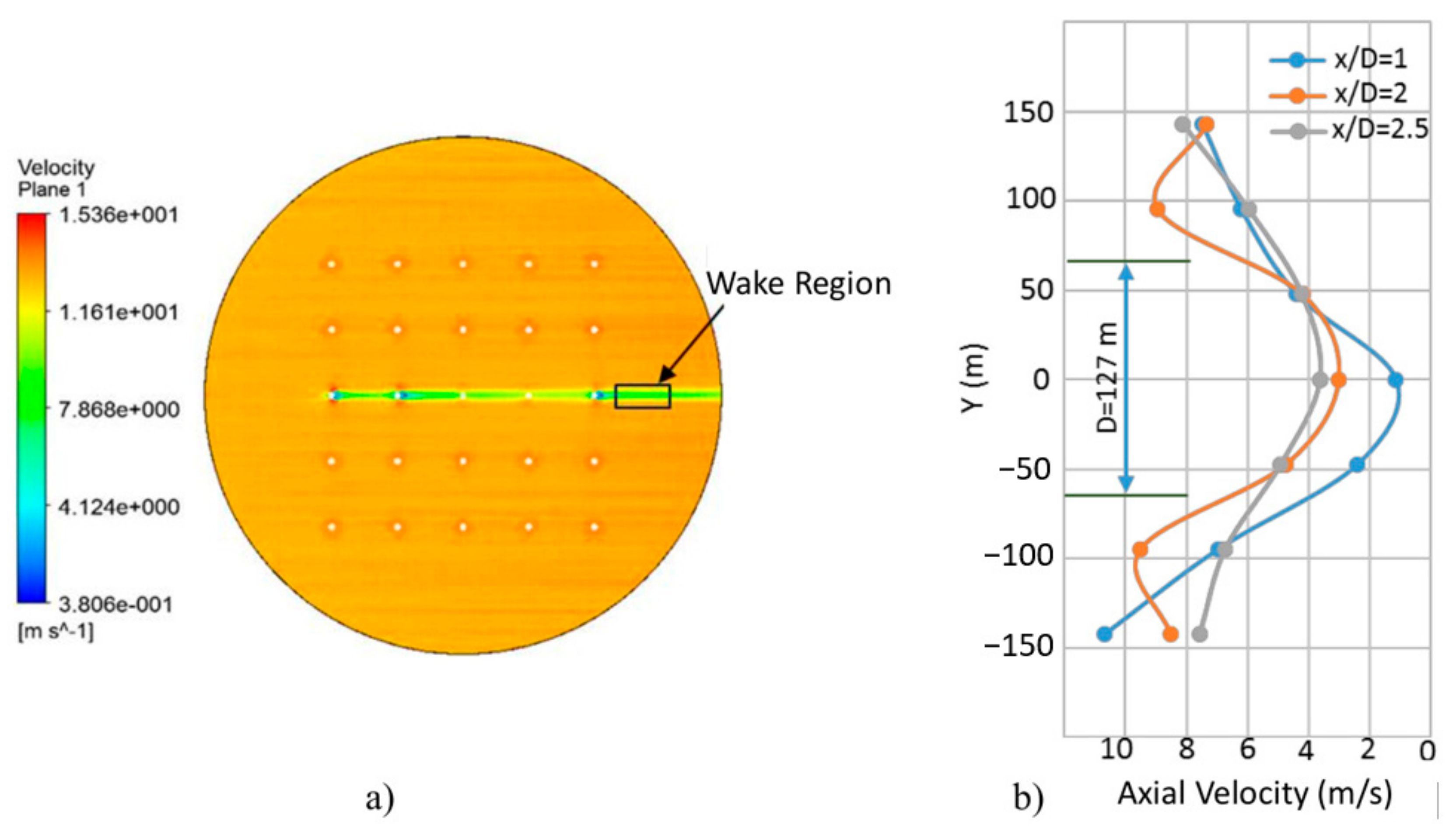
2. Fluid Field Simulation in Wind Farm

The flow field in the wake region behind offshore wind turbines is characterized by a significant reduction of wind velocity and increased level of turbulence intensity. The interaction between the wind turbine and the turbulent flow field generates complex flow characteristics combined with a number of aerodynamic effects. Because it is a non-linear and three-dimensional process, the difficulty arises when the measurement has to include the three-dimensional wind velocity vector at all the time and all the position in the wake region [27]. There are a number of instruments for turbulence measurement. Among them, the sonic anemometer is currently the most popular in situ instrument which can continuously measure the three-dimensional flow. However, it is not suitable to measure the wake flows because of the difficulty to cover a big volume when mounting them on the meteorological masts. Recently, a promising remote sensing technique using a wind-speed Doppler light detection and ranging (Lidar) was used for full-field wake measurements [28]. The Lidar system uses pulsed scanning long-range devices that can capture many simultaneous measurements along the laser beam. It could provide high accuracy, relatively high spatial resolution, and long range. The drawback of the Lidar technique is that it can only measure the velocity component parallel to the laser beam. Therefore, it is very difficult to reconstruct the horizontal wind vector with a single Lidar. Many uncertainties due to the local variability of the wind direction will affect the reconstruction of the horizontal wind vector that tends to grow infinitely when the Lidar measures perpendicular to the wind direction. This is the limitation of Lidar when measuring the wind turbine wake [29]. Multiple Lidar techniques that can scan over the same area of interest from different locations could overcome this limitation, but they are too expensive and require a significantly higher degree of expertise to be properly operated [30]. Use of two Lidars has shown that wake has a fast recovery rate in convective atmospheric conditions, a setup comprising two long-range Lidar devices was introduced to measure the inflow and wake flow [31]. Moreover, the speed of the measurement is another limitation of the Lidar techniques. The scanning process emits thousands of laser pulses in a particular direction, examines the pulses bounce signal, calculates the Doppler shift at different distances, and continuously proceeds to the next laser beam [27]. Beck et al. introduced a technique using long-range Lidar measurements reconstruction of three-dimensional dynamic wind-turbine wake wind fields. However, it is not feasible to volumetrically measure wakes on appropriate time scales because of the limited scanning speeds of long-range Lidar [28]. Wildmann et al. used the Doppler wind Lidar velocity-azimuth display (VAD) scans to retrieve the turbulence kinetic energy dissipation rate [32]. It showed that the Lidar parameters such as the pulse width of the laser beam and the Lidar time window could reduce the uncertainty of the model functions and improve the corrections of the volume-averaging effects. However, those two parameters may differ for individual Lidar. Furthermore, the turbulence kinetic energy dissipation rate could be retrieved using VAD scans with a larger elevation angle.

As a result, the aforementioned full-field wake measurements need much more experience in the application of Lidar measurements and they are by far too expensive or not easy to apply for onshore and offshore. Although, the probe volume of a Lidar influences the wind speed, and even the feasibility of the Lidar system to measure the turbulence flow is still in the dispute. However, we tried to relate the wind turbine failure with the mean wind speed of the wake region by the computational fluid dynamics (CFD) simulation in this study. It is assumed that the mean wake flow speed can be measured, and Lidar is just one of the equipment.

2.1. Governing Equations and Numerical Method

In this study, the wind energy dissipation model was coupled with flow dynamics to evaluate the fluid field of the wind farm. The simulation of the CFD was realized by the commercial software Fluent. Then, the wind velocity and direction in the wind field simulation were exported for the wind turbine fault detection. This program solved the pressure-based steady 3D Navier–Stokes equations, including the continuity Equation (1) and momentum Equation (2) [33,34]:

$$\nabla .\rho V=0,$$

(1)

$$\rho V.\nabla V=-\nabla p+\mu {\nabla }^{2}V+S,$$

(2)

where $\nabla$ is the divergence, $\rho$ is the density, $p$ is the pressure, and V is the velocity. In the present study, the source term, S, was used to simulate the energy loss when the wind flew into the wind turbine. In this simulation, the wind speed was calculated by using steady Navier–Stokes equations and the air density was set to 1.225 $\mathrm{kg}/$m³. Because the air density is subject to change with temperature, humidity, and pressure, it needs to be determined by the air density normalization equation when applying the real-world measurement data to the simulation [35]. According to Betz’s law, no turbine can capture more than 16/27 (~59%) of the kinetic energy in wind [36]. Therefore, this study assumed that wind turbine got 59% energy from the wind, and the wind energy loss only resulted in the reduction of the wind velocity. As a result, the source term is derived base on energy balance and Betz’s law described defined by Equation (3):

$$S=-0.7\rho V\left|V\right|.$$

(3)

The solver used the least squares cell based finite volume method with a second order upwind discretization scheme. In addition, the standard $k-\epsilon$ turbulence model with a standard wall function was used to deal with the closure problem [33,34,37,38]. Furthermore, the pressure velocity linkage was solved via the coupled scheme [33,34]. Additionally, the source term equation was written in a C language program, and added into the CFD model by the Fluent user-defined function (UDF) [39].

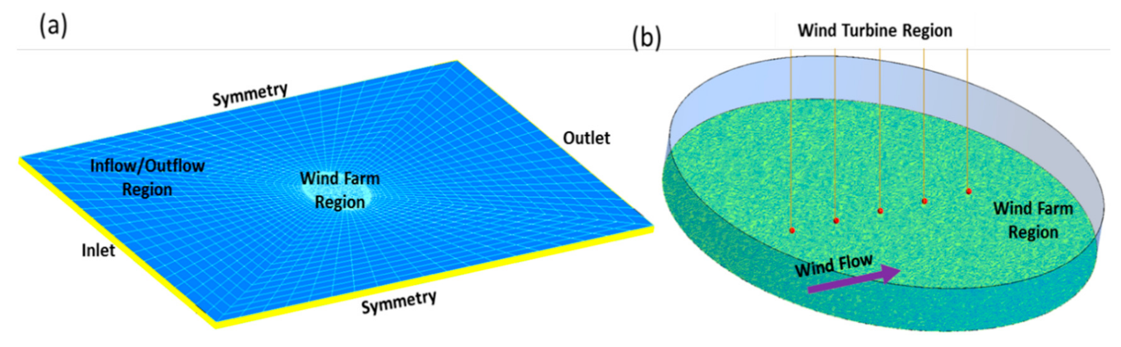
2.2. Computational Domain and Simulation Conditions

Because the 3D Navier–Stokes equation was solved in steady state, only one simulation was required for each boundary condition. The wind speed was set from 4 to 20 m/s, the turbulence intensity was set to 0.1, and the wind direction was aligned with the wind turbine array. A total number of 272 simulations were conducted including the conditions of fault-free, single turbine fault, and multiple turbine faults. The computational domain mesh layout and boundary conditions are shown in Figure 2a. The geometry of the computational domain was divided into three parts, namely, the inflow/outflow region, the wind farm region, and the wind turbine regions. Wind turbine region areas were used for simulating wind turbine energy capture. As shown in Figure 2b, five wind turbine regions were located along a line parallel to the inflow wind direction. On the other hand, the wind turbine regions were set in the wind farm region, and the wind farm region was set in the middle of the inflow/outflow region. The geometry of the inflow/outflow region consisted of cuboids, and the length, width, and height were 80,000, 48,000, and 500 m, respectively. The wind farm region geometry consisted of a 10,000 m diameter cylinder, the height of which was the same as the height of the inflow/outflow region. In addition, a spherical wind turbine region was used to describe the characteristics of the energy captured by the wind turbine. In this study, the spheres’ diameter was set to 127 m to simulate the diameter of a wind turbine. In addition, the distance between the spherical center and the base of the computational domain was set to 100 m, which simulated the hub height of the wind turbine. Finally, the distance between two adjacent wind turbines was set to 1270 m, to simulate the distance between two adjacent spherical wind turbine regions.

The computational domain employed a hybrid grid system, and the total number of elements was 1,130,000. Moreover, the structured mesh consisted of the inflow/outflow region of the computational domain, and the unstructured mesh comprised the other parts. On the other hand, the source term of the governing equations was only applied to the wind turbine regions to simulate the wind energy loss, which was caused by energy captured by the wind turbine. The inlet boundary condition assumed that the power law wind profile is defined by the following equation:

$$u\left(\mathrm{z}\right)=u_0{\left(\frac{z}{z_r}\right)}^{\alpha },$$

(4)

where $u\left(z\right)$ is the vertical wind velocity profile and $u_0$ is the velocity at the reference height of $z_r$. The exponent α is 0.11 for wind flow over open water area [40]. In the present study, 5% turbulence intensity and a 127 m hydraulic diameter in the free stream were assumed in order for $k$ and $\epsilon$ at the inlet boundary to be estimated [34]. The fixed pressure outlet boundary condition was used. In addition, the symmetry boundary condition was applied to the two side walls and the top wall of the computational domain. Besides, the no-slip wall boundary condition was set on the base wall.

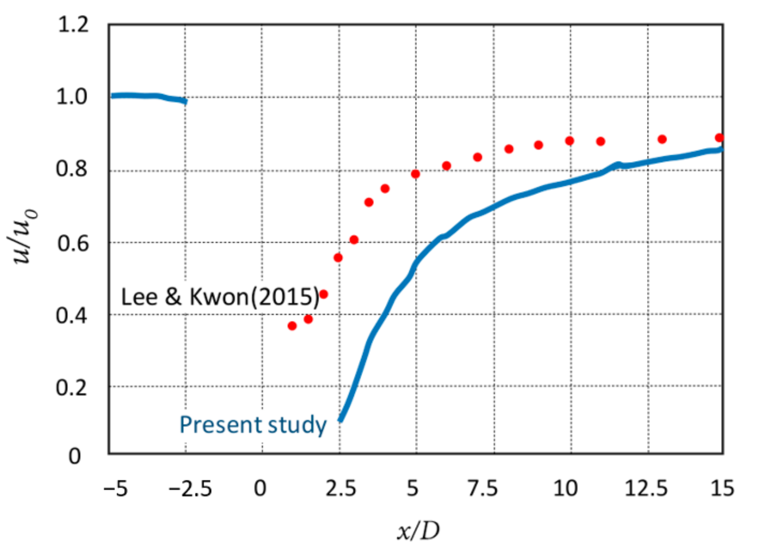
2.3. Validation of Source Term

The commercial CFD package was extensively verified, and the flow kinetic energy loss model in the turbine region was added in this study. That model was not included in the commercial package verification. In this section, the single wind turbine simulation with the flow kinetic energy loss model is discussed to verify the source term. By using this source term, the results showed that the wind velocity was reduced after the wind flew through the wind turbine, as shown in Figure 3. As the distance from the wind turbine increases, the wind velocity approaches the free stream velocity. Such qualitative results are consistent with the actual characteristics of the wind measured at the wind turbine wake side [24,25,26]. When compared to the quantitative results, the wake velocity recovery ability of the simulation is lower than that of the actual measurement [41]. This means that the wind energy captured by the wind turbine in the simulation may be higher than that in real cases.

When the computational domain is configured as shown in Figure 2, the normalized stream-wise wind velocity along the wind turbine array at hub height will be as shown in Figure 4, which illustrates the characteristic of the velocity at hub height when the wind flow passes through multiple wind turbines. When the wind passes through the first wind turbine, the behavior of the wake characteristic of the wind turbine is as shown in Figure 3. However, the wind will enter the second wind turbine even though the wind speed has not yet recovered to the free-flow wind speed; therefore, the entrance wind speed is also relatively low. The proposed wind energy dissipation model in this study will also reduce the energy dissipated from the wind farm, and the following flow field will have similar characteristics. As the wind flow passes through more wind turbines, the characteristics of the wind field will become much more similar, and so does the flow field characteristics to the spatial fully developed.

In this paper, we assumed that the wind turbine can reach the Betz’s limit in the flow kinetic energy loss model. However, the captured wind turbine energy is always lower than the Betz’s limit in the wind energy conversion. This could be caused by failing to consider the change of wind velocity in the swirl direction. In addition, the turbine’s nacelle and tower were not considered in this simulation. These three reasons may cause the difference between the simulation and measurement results.

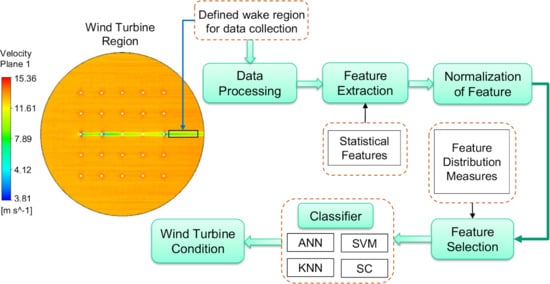
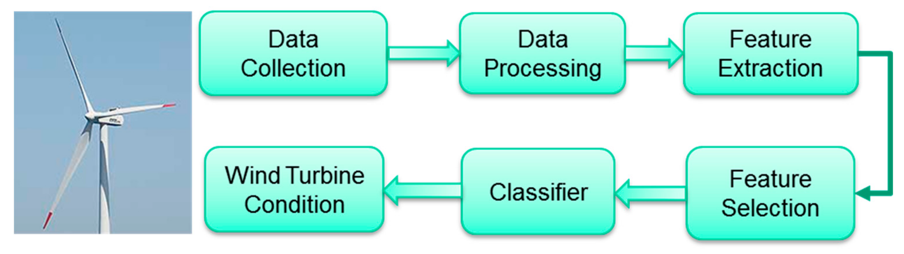
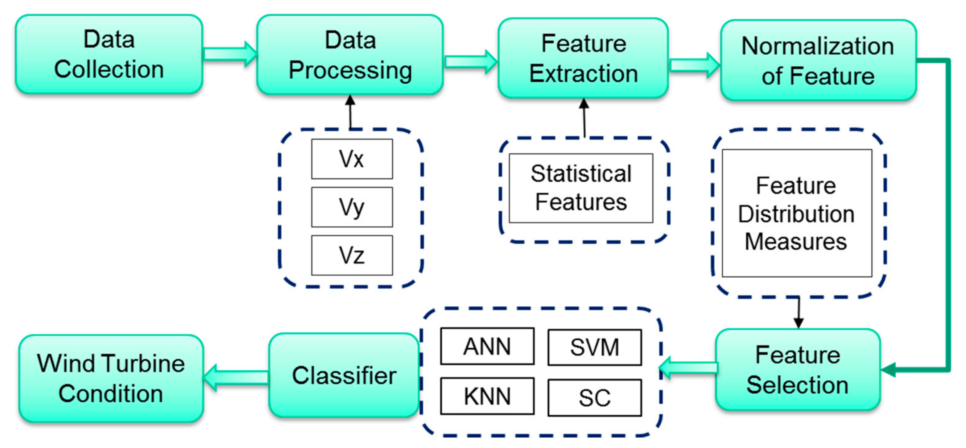
3. Wind Farm Fault Detection Methodology

3.1. Overview

In this study, a new method is proposed to detect wind turbine faults based on the decrease of wind speed in the wake region behind a wind farm. The approach can detect not only single wind turbine faults but also multi-wind turbine faults. Figure 5 shows the flow chart of the approach. Firstly, wind speed signals are collected from the wake regions, which are defined by a width of 2.4 D and a distance of 1–3 D behind the last wind turbine, owing to the high disturbance and velocity profiles in this region. The wake region was defined previously to ensure that the small number of measurement points can represent the maximum wake deficit of the last wind turbine in the wind farm. The statistical features that represent significant relevance to the wind turbine condition are then extracted from the wind speed. A novel feature selection algorithm based on the distance between feature distributions is proposed to achieve high classification accuracy. Finally, several artificial machine learning methods are applied to identify wind turbine conditions.

3.2. Feature Extraction

Figure 6a represents the simulation result from the top view of wind farm, in which the wind speed in the wake region on the x-y plane was simulated. Figure 6b shows the wind turbine velocity deficit profile in the wake region along the horizontal-axis in terms of three distances behind the wind farm. They all have the largest velocity difference near the center, and the velocity difference decreases with the increase of the distance in the wake region. Statistical indexes were then applied to the wind speeds in x, y, and z directions to extract features for future feature selection. These indexes were determined using Equations (5)–(8):

$$\mathrm{RMS} =\sqrt{\frac{1}{n}{{\displaystyle \sum }}_{i=1}^n{x}_i^2} ,$$

(5)

$$\mathrm{Standard}\mathrm{Deviation}\left(\mathrm{STD}\right)=\sqrt{\frac{1}{n}{{\displaystyle \sum }}_{i=1}^n{\left(x_i-\overline{x}\right)}^2},$$

(6)

$$\mathrm{Variance}=\frac{1}{n}{{\displaystyle \sum }}_{i=1}^n{\left(x_i-\overline{x}\right)}^2,$$

(7)

$$\mathrm{Kurtosis}=\frac{1}{n}{{\displaystyle \sum }}_{i=1}^n{\left(\frac{x_i-\overline{x}}{STD}\right)}^4,$$

(8)

where n is the number of samples and $x_i$ is the value of the wind speed.

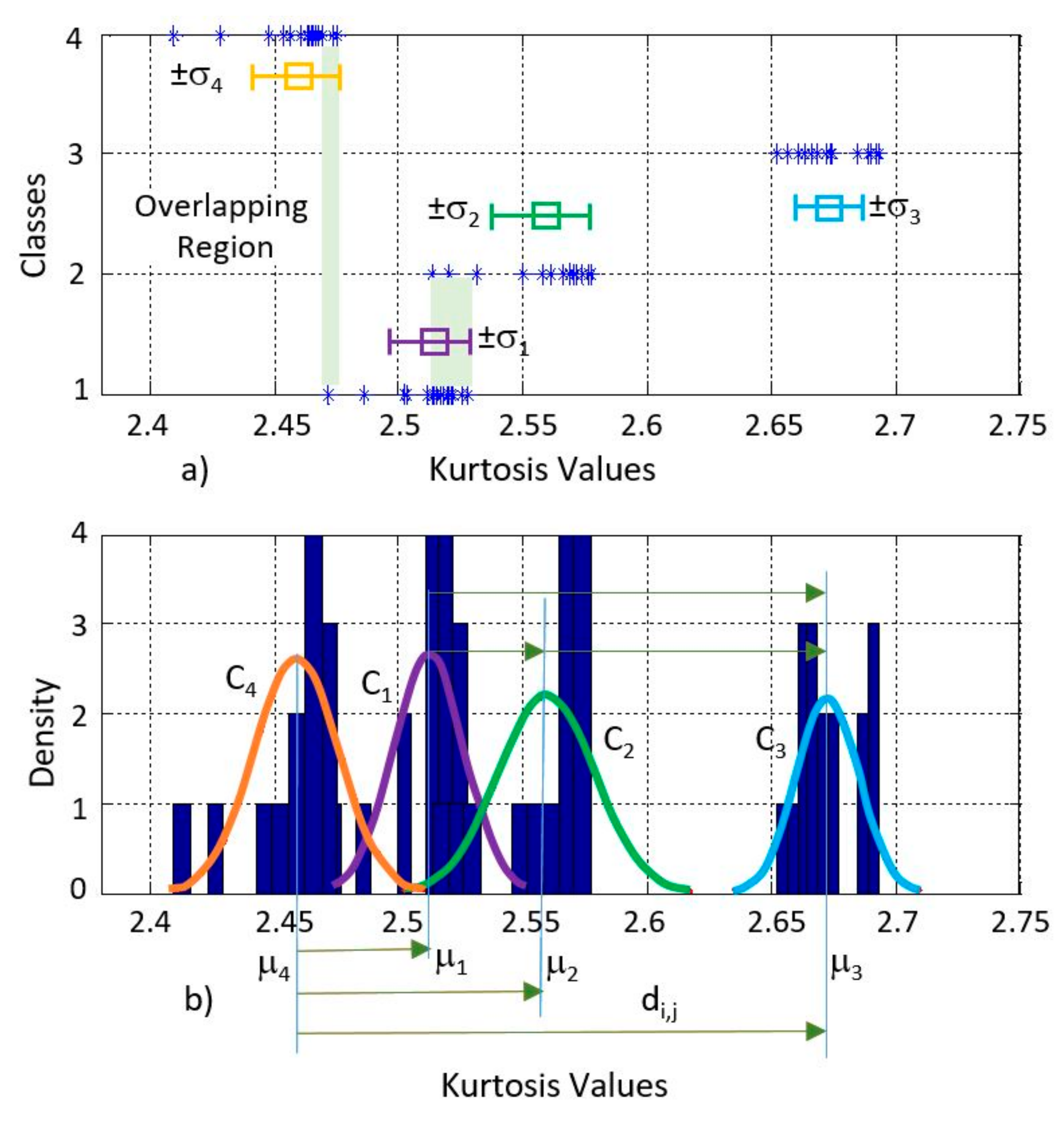
3.3. Feature Selection

Feature selection is a process aiming to select a subset of features, which have significant relevance to the decision-making process. In other words, irrelevant and redundant features could be detected and removed through the selection process. Thus, the accuracy of the predictive model can be improved, and the number of measurements and learning time reduced [42,43]. Feature selection provides many advantages, particularly when we are working with a large amount of data. As wind speed varies in the wake region, we need to consider the distribution of the extracted features in each class. Figure 7 shows the distribution of Kurtosis values of wind speed in the x direction in terms of four classes. The first class represents all wind turbines in good condition. The rest of the three classes represent three cases of single fault. They are the first wind turbine, the second wind turbine, and the third wind turbine fault, respectively. The ratio of the distance between the two mean distribution values and a total of two STDs can provide significant information about how the subset is relevant to the original database. This ratio is accounted for in the proposed feature selection algorithm to remove the irrelevant features and rank the selected features.

In this study, we proposed a new feature selection method considering feature distribution in each class shown in Figure 7. We assume that the set of features of the original data $D_{m\times n}$ is $X=\left[x_1, x_2,\dots x_n\right]$ and the class set is represented as $C=\left[c_1, c_2,\dots c_n\right]$. The feature selection algorithm involves the following steps:

(1)

From the normal distribution of feature $x_l$ into each class $c_i$, calculate the mean values ${\mu }_{l,i}$ and STDs ${\sigma }_{l,i}$ for each group.

(2)

Calculate the distance between every two groups for each feature based on the mean values:

$$d_{i,j}=\left|{\mu }_i-{\mu }_j\right|\mathrm{for}i=1:k-1\mathrm{and}j=2:k,i\ne j,$$

(9)

$${\sigma }_{i,j}=\left|{\sigma }_i-{\sigma }_j\right|\mathrm{for}i=1:k-1\mathrm{and}j=2:k,i\ne j.$$

(10)

(3)

Check probability overlapping in the significant range using the ratio of $d_{i,j}/{\sigma }_{i,j.}$

(4)

Rank the features following the condition:

$$P_l=\sum p_{i,j} \mathrm{where}{p}_{i,j}=\left\{\begin{array}{c}1, if \frac{d_{i,j}}{{\sigma }_{i,j}}\ge 1\\ 0, if 0.5<\frac{d_{i,j}}{{\sigma }_{i,j}}<1\\ -1, otherwise\end{array}\right..$$

(11)

(5)

Remove irrelevant features that have a small value of $P_l:P_l<threshold.$

3.4. Artificial Machine Learning Classifiers

The SC is a classifier based on the fuzzy similarity in the Lukasiewicz structure; it was first introduced by Luukka [44]. This structure has a strong connection to the first-order logic. Suppose a data set $X$ will be classified into N different classes across 𝑛 features of $\left(f_1, f_2,\dots ,f_n\right)$. The procedure of the SC begins with the definition of an ideal vector for each class. The ideal vector $I_i=\left[I\left(1\right),I\left(2\right),\dots ,I\left(N\right)\right]$, which represents the class $C_i$ in the best way possible, can be determined from the sample set $x=\left[x\left(1\right),x\left(2\right),\dots ,x\left(N\right)\right]$, using the generalized mean described in Equation (12). In which, the power $m$ is fixed $\forall i, r$ and $\#X_i$ is the number of samples in the class $C_i$. Then, the data vector is compared to the ideal vector and the similarities $S\left(x,I\right)$ are determined using a generalized Lukasiewicz structure in Equation (13). Finally, the decision whether $x$ belongs to class $C_k$ is made according to the highest similarity value, which is calculated using Equation (14). Where the parameter $p, m$, and the weights $w_r \in \left[0, 1\right]$ for each dimension are fixed:

$$I_r={\left(\frac{1}{\#X_i}{{\displaystyle \sum }}_{x\in X_i}x{\left(r\right)}^m\right)}^{1/m},\forall r=1:n,$$

(12)

$$S\left(x,I\right)={\left(\frac{1}{n}{{\displaystyle \sum }}_{r=1}^n{w}_r{\left(1-\left|x{\left(r\right)}^p-I{\left(r\right)}^p\right|\right)}^{m/p}\right)}^{1/m},$$

(13)

$$S\left(x,I_k\right)=max\left\{S\left(x,I_i\right)\right\},i=1:N.$$

(14)

The KNN is the other method used to classify the wind turbine faults in this study. KNN is a simple algorithm based on feature similarity like the distance function. With a given positive integer $k$, the distance $d$ between an unseen observation $x$ and each training observation $x^{\prime }$ can be obtained using Equation (15). The conditional probability, $P,$ is then estimated for each class using Equation (16). Finally, the input x gets assigned to the class with the largest probability:

$$d\left(x,x^{\prime }\right)=\sqrt{{\left(x_1-x_1^{\prime }\right)}^2+{\left(x_2-x_2^{\prime }\right)}^2+\dots +{\left(x_n-x_n^{\prime }\right)}^2},$$

(15)

$$P\left(Y=j|X=x\right)=\frac{1}{k}\sum I\left(y_i=j\right),$$

(16)

where $I\left(y_i=j\right)=\left\{\begin{array}{c}1, if y_i=j:true\\ 0, otherwise\end{array}\right.$.

An ANN is a set of interconnected nodes called neurons. It is one of the commonly-used candidates for solving classification problems. Particularly, ANN is well suited for complex decision boundary problems over many variables. A single neuron in the ANN model represents the relationship between a given set of inputs and outputs; it is described in Equations (17) and (18):

$$\widehat{y_i}=f\left[{\displaystyle \sum }_{i=1}^n{w}_i.x_i-\theta \right],$$

(17)

$$f\left(x\right)=\frac{1}{1+e^{-x}},$$

(18)

where $\widehat{y_i}$ is the output, $x_i$ is the input set, $w_i$ is the weight between neurons, $\theta$ is the threshold, and $f\left(x\right)$ is the sigmoid function which is used as the activation function. In this study, a single hidden layer of 10 neurons was applied for training the network. SVM is another method used in this study, and it is an effective machine learning method for classification problems. SVM-based classification determines an optimal separating hyper plane, which is characterized by a maximum separation to the closest training points. The advantage of SVM over other classifiers is that it could deal with the issues in the training process such as over-fitting and local minima. In addition, it requires a small sample of training vectors. Further details of the SVM algorithm were introduced by Vapnik [45]. In this study, the Gaussian kernel was used to implement kernel SVM to construct the optimal separating hyper plane between the classes.

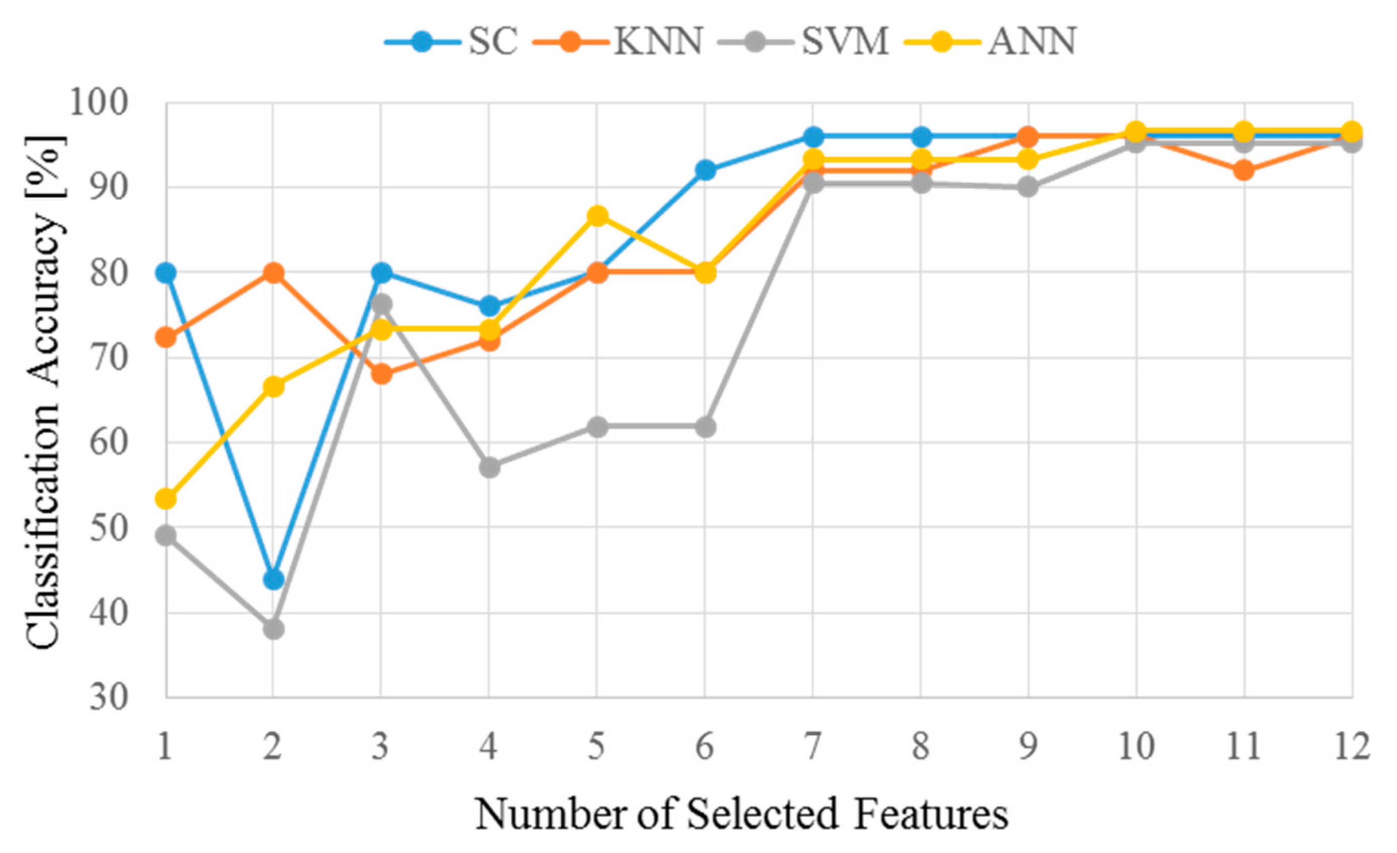
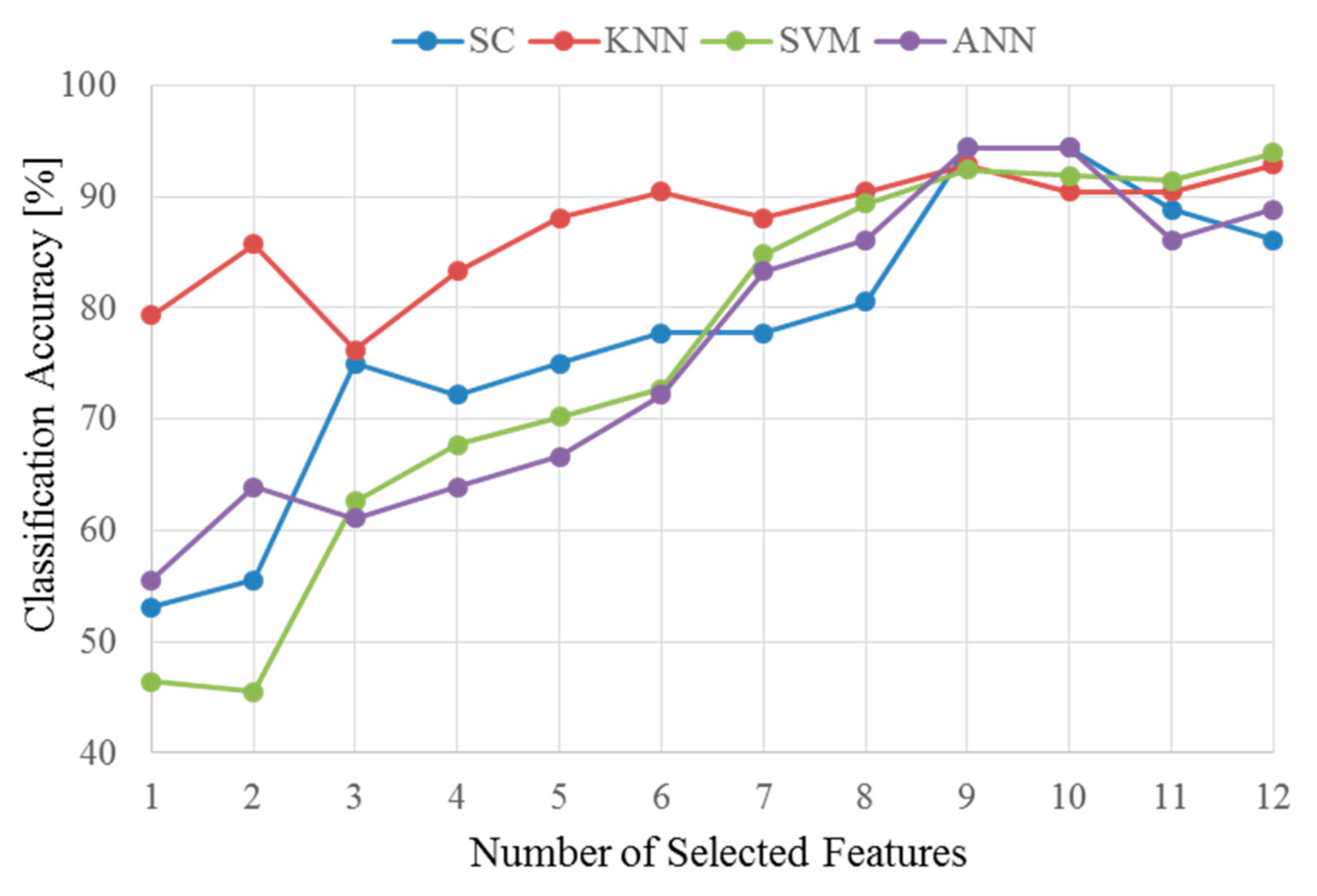
4. Results and Discussions

Simulation results of wind speeds presented in the previous section were used to generate the training and testing data for the condition monitoring of the wind turbines. In this study, the status of five wind turbines including health, single fault, and multi faults were detected using artificial machine learning methods with feature selection. There are six combinations for single wind turbine fault detection and sixteen combinations for single and two-wind turbine fault detection. Twelve features including RMS, STD, variance, and Kurtosis of the wind speed in the x, y, and z directions were extracted from the original dataset. The feature selection method based on feature distribution was applied to eliminate irrelevant features, and the remaining selected features were ranked according to their scores. All data were normalized and randomly split into an 82% training set and an 18% testing set. Single wind turbine fault detection results are shown in Figure 8. When the number of selected features is fewer than seven, it could be seen that SVM provides the lowest classification accuracy. Whereas, all machine learning techniques show high accuracy once the number of selected features is larger than seven. Furthermore,

Table 1. Classification Accuracy for a Single Fault.

Selected Feature	SC (%)	KNN (%)	SVM (%)	ANN (%)
4	76	72	57.14	73.33
all	96	96	95.23	96.67
10	96	96	95.23	96.67

verifies that even if the number of features is reduced, the highest classification accuracies remain at approximately 96%. This implies that there are several irrelevant and redundant subsets of wind speeds that need to be removed to reduce computational time.

Figure 9 illustrates the results of multi-fault detection using different classifiers, in which the number of classes reaches sixteen, which includes six classes of single fault and ten classes of two combination faults. It can be seen that even if more wind turbine faults occur, high classification accuracies can be achieved. In this case, when a small number of features were selected, ANN and SVM classifiers provided lower classification accuracies compared to that provided by KNN and SC. However, they represented good classification results once a larger number of features were selected. The highest classification accuracies obtained were approximately 94% using nine selected features. However, the inclusion of all selected features may cause the decrease of classification accuracy, as shown in

Table 2. Classification Accuracy for Multi-Fault.

Selected Feature	SC (%)	KNN (%)	SVM (%)	ANN (%)
3	75	76.19	62.62	61.11
all	88.09	90.47	88.09	90.47
9	94.44	92.86	92.42	94.44

. Through the feature selection algorithm, the three most important features were Kurtosis indexes of wind speed in the x, y, and z directions. On the other hand, RMS indexes of wind speed in the y and z directions and the variance index in the z direction were the three most irrelevant and redundant features. Those irrelevant features were removed to obtain better classification performance, reduce storage and computational time, and generalize interpretable models.

To validate the proposed feature selection algorithm, the rankings of all features obtained from different feature selection algorithms are shown in

Table 3. Feature ranking by different feature selection methods.

Rank	FEM	RFE	New Method
1	STD_y	Kur_z	Kur_x
2	Kur_y	STD_y	Kur_y
3	Var_x	STD_x	Kur_z
4	RMS_x	Var_y	STD_y
5	STD_z	Var_x	STD_z
6	STD_x	STD_z	Var_x
7	Kur_z	Kur_y	RMS_x
8	RMS_y	RMS_x	STD_x
9	Kur_x	Kur_x	Var_y
10	RMS_z	Var_z	RMS_y
11	Var_y	RMS_y	RMS_z
12	Var_z	RMS_z	Var_z

. Two other feature selection methods, fuzzy entropy measures (FEM) [44] and recursive feature elimination methods (RFE) [46], were applied to justify the proposed feature selection method.

Figure 10 illustrates multi-fault classification accuracies using the KNN classifier with different feature selection methods. The selected features are ranked in Table 3. The figure shows that higher classification accuracies are obtained when larger number of features are selected. When the number of selected features is 7, 8, and 10, the classification results from the three feature selection methods are in a good agreement. Whereas, for the other cases, the proposed feature selection shows slightly higher accuracies compared to the two other methods. The best classification accuracy can be obtained with nine selected features.

5. Conclusions

A novel perspective regarding fault detection of wind farm turbines was proposed in this research. A wind energy dissipation model was coupled with a computational fluid dynamics solver to simulate the fluid field of a wind turbine array, and the wind velocity and direction in the simulation were exported for identifying wind turbine fault. The simulation result shows the feasibility of detecting single and multiple faults in a wind turbine array by using the wind speed in the wake region. This method has the advantage over conventional fault detection methods installed on individual wind turbines in terms of cost and convenience. The contributions of this research could be summarized as follows:

• A wind farm model was presented by adding the flow kinetic energy loss model in the turbine region. This model was able to simulate the nonlinear wind field without the information of thrust force. The simulation result was qualitatively consistent with the actual characteristics of the wind measured at the turbine wake side.
• A new feature selection algorithm specifically designed for the wind speed monitoring was proposed. Due to the volatile characteristic of wind flow, this algorithm took the distribution of the features into account and ranked them in terms of their relevance to the classification. The proposed algorithm proved to have a better performance than the FEM and RFE under a limited feature number.
• The faults in a wind turbine array were detected by measuring the wind velocity difference in the wake region. The performance of several machine learning methods, such as SC, KNN, SVM, and ANN, were presented and compared. It was confirmed that 96% accuracy could be achieved for single fault detection with 10 selected features, and 94.44% accuracy could be achieved for two-fault detection with 9 selected features.
• The success of the novel fault detection scheme presented in this study provides significant potential for remote monitoring and diagnosis of offshore wind farms. Not only single fault but also multi-faults in wind turbines can be well detected by measuring the wind speed.

In addition to prediction of the wind farm fault, the results also can be used to determine the wind loads on the blade. The wind action can be used to develop the fragility curve to estimate the probability of failure of the wind turbine-supporting structures [47]. Thus, the performance of the wind turbine tower at selected locations will be fully investigated in the future work.

References

1. Ladenburg, J. Attitudes towards on-land and offshore wind power development in Denmark; choice of development strategy. Renew. Energy 2008, 33, 111–118. [Google Scholar]
2. Christensen, J.J.; Andersson, C.; Gutt, S. Remote condition monitoring of Vestas turbines. In Proceedings of the European Wind Energy Conference, Marseille, France, 16–19 March 2009; pp. 1–10. [Google Scholar]
3. Yang, S.; Li, W.; Wang, C. The intelligent fault diagnosis of wind turbine gearbox based on artificial neural network. In Proceedings of the International Conference on Condition Monitoring and Diagnosis, Beijing, China, 21–24 April 2008; pp. 1327–1330. [Google Scholar]
4. Bennouna, O.; Héraud, N.; Camblong, H.; Rodriguez, M. Diagnosis of the Doubly-Fed Induction Generator of a Wind Turbine. Wind. Eng. 2005, 29, 431–447. [Google Scholar]
5. Widodo, A.; Kim, E.Y.; Son, J.-D.; Yang, B.-S.; Tan, A.C.; Gu, D.-S.; Choi, B.-K.; Mathew, J. Fault diagnosis of low speed bearing based on relevance vector machine and support vector machine. Expert Syst. Appl. 2009, 36, 7252–7261. [Google Scholar]
6. Caselitz, P.; Giebhardt, J.; Krüger, T.; Mevenkamp, M. Development of a fault detection system for wind energy converters. In Proceedings of the European Union Wind Energy Conference, Göteborg, Sweden, 20–24 May 1996; pp. 1004–1007. [Google Scholar]
7. Guo, P.; Infield, D.; Yang, X. Wind Turbine Generator Condition-Monitoring Using Temperature Trend Analysis. IEEE Trans. Sustain. Energy 2011, 3, 124–133. [Google Scholar]
8. Qiao, W.; Lu, D. A Survey on Wind Turbine Condition Monitoring and Fault Diagnosis—Part II: Signals and Signal Processing Methods. IEEE Trans. Ind. Electron. 2015, 62, 6546–6557. [Google Scholar]
9. Hameed, Z.; Hong, Y.; Cho, Y.; Ahn, S.-H.; Song, C. Condition monitoring and fault detection of wind turbines and related algorithms: A review. Renew. Sustain. Energy Rev. 2009, 13, 1–39. [Google Scholar]
10. Nie, M.; Wang, L. Review of Condition Monitoring and Fault Diagnosis Technologies for Wind Turbine Gearbox. Procedia CIRP 2013, 11, 287–290. [Google Scholar]
11. Koulocheris, D.; Gyparakis, G.; Stathis, A.; Costopoulos, T. Vibration Signals and Condition Monitoring for Wind Turbines. Engineering 2013, 5, 948–955. [Google Scholar] [CrossRef] [Green Version]
12. Igba, J.; Alemzadeh, K.; Durugbo, C.; Eiriksson, E.T. Analysing RMS and peak values of vibration signals for condition monitoring of wind turbine gearboxes. Renew. Energy 2016, 91, 90–106. [Google Scholar] [CrossRef] [Green Version]
13. Jin, X.; Qiao, W.; Peng, Y.; Cheng, F.; Qu, L. Quantitative Evaluation of Wind Turbine Faults Under Variable Operational Conditions. IEEE Trans. Ind. Appl. 2016, 52, 2061–2069. [Google Scholar] [CrossRef]
14. Cheng, F.; Peng, Y.; Qu, L.; Qiao, W. Current-based Fault Detection and Identification for Wind Turbine Drivetrain Gearboxes. In Proceedings of the IEEE Industry Applications Society Annual Meeting, Portland, OR, USA, 2–6 October 2016. [Google Scholar]
15. Salameh, J.P.; Cauet, S.; Etien, E.; Sakout, A.; Rambault, L. Gearbox condition monitoring in wind turbines: A review. Mech. Syst. Signal Process. 2018, 111, 251–264. [Google Scholar] [CrossRef]
16. Lu, B.; Li, Y.; Wu, X.; Yang, Z. A review of recent advances in wind turbine condition monitoring and fault diagnosis. In Proceedings of the 2009 IEEE Power Electronics and Machines in Wind Applications, Lincoln, NE, USA, 24–26 June 2009; pp. 1–7. [Google Scholar] [CrossRef]
17. Kabir, M.J.; Oo, A.M.T.; Rabbani, M. A Brief Review on Offshore Wind Turbine Fault Detection and Recent Development in Condition Monitoring Based Maintenance System; Institute of Electrical and Electronics Engineers: New York, NY, USA, 2015; pp. 1–7. [Google Scholar]
18. Lu, W.; Chu, F. Condition monitoring and fault diagnostics of wind turbines. In Proceedings of the 2010 Prognostics and System Health Management Conference, Macau, China, 12–14 January 2010; pp. 1–11. [Google Scholar]
19. Menke, R.; Vasiljević, N.; Hansen, K.S.; Hahmann, A.N.; Mann, J. Does the wind turbine wake follow the topography? A multi-lidar study in complex terrain. Wind Energy Sci. 2018, 3, 681–691. [Google Scholar] [CrossRef] [Green Version]
20. Kermani, A.; Andersen, S.; Sørensen, N.; Shen, W. Analysis of turbulent wake behind a wind turbine. In Proceedings of the International Conference on Aerodynamics of Offshore Wind Energy Systems and Wakes, Copenhagen, Denmark, 17–19 June 2013. [Google Scholar]
21. Schümann, H.; Pierella, F.; Saetran, L. Experimental Investigation of Wind Turbine Wakes in the Wind Tunnel. Energy Procedia 2013, 35, 285–296. [Google Scholar]
22. Ainslie, J. Calculating the flowfield in the wake of wind turbines. J. Wind. Eng. Ind. Aerodyn. 1988, 27, 213–224. [Google Scholar]
23. Talmon, A.M. The Wake of a Horizontal-axis Wind Turbine Model. Measurements in Uniform Approach Flow and in a Simulated Atmospheric Boundary Layer; Report 85-010121, TNO Apeldoorn; TNO Division of Technology for Society Technology: The Hague, The Netherlands, 1985. [Google Scholar]
24. Göçmen, T.; Van der Laan, P.; Réthoré, P.E.; Diaz, A.P.; Larsen, G.C.; Ott, S. Wind turbine wake models developed at the technical university of Denmark: A review. Renew. Sustain. Energy Rev. 2016, 60, 752–769. [Google Scholar]
25. Sedaghatizadeh, N.; Arjomandi, M.; Kelso, R.; Cazzolato, B.S.; Ghayesh, M.H. Modelling of wind turbine wake using large eddy simulation. Renew. Energy 2018, 115, 1166–1176. [Google Scholar]
26. Hansen, M.O.L. Aerodynamics of Wind Turbine, 2nd ed.; Earthscan Publication Ltd.: London, UK, 2008. [Google Scholar]
27. Fuertes, F.C.; Porté-Agel, F. Using a Virtual Lidar Approach to Assess the Accuracy of the Volumetric Reconstruction of a Wind Turbine Wake. Remote Sens. 2018, 10, 721. [Google Scholar]
28. Beck, H.; Kühn, M. Reconstruction of Three-Dimensional Dynamic Wind-Turbine Wake Wind Fields with Volumetric Long-Range Wind Doppler LiDAR Measurements. Remote Sens. 2019, 11, 2665. [Google Scholar]
29. Bromm, M.; Rott, A.; Beck, H.; Vollmer, L.; Steinfeld, G.; Kühn, M. Field investigation on the influence of yaw misalignment on the propagation of wind turbine wakes. Wind Energy 2018, 21, 1011–1028. [Google Scholar]
30. Newman, J.F.; Bonin, T.; Kastner-Klein, P.; Wharton, S.; Newsom, R.K. Testing and validation of multi-lidar scanning strategies for wind energy applications. Wind Energy 2016, 19, 2239–2254. [Google Scholar]
31. Van Dooren, M.F.; Trabucchi, D.; Kühn, M. A Methodology for the Reconstruction of 2D Horizontal Wind Fields of Wind Turbine Wakes Based on Dual-Doppler Lidar Measurements. Remote Sens. 2016, 8, 809. [Google Scholar]
32. Wildmann, N.; Päschke, E.; Roiger, A.; Mallaun, C. Towards improved turbulence estimation with Doppler wind lidar velocity-azimuth display (VAD) scans. Atmos. Meas. Tech. 2020, 13, 4141–4158. [Google Scholar]
33. ANSYS. ANSYS FLUENT 14.0 Theory Guide; ANSYS, Inc.: Canonsburg, PA, USA, 2011. [Google Scholar]
34. ANSYS. ANSYS FLUENT 14.0 User’s Guide; ANSYS, Inc.: Canonsburg, PA, USA, 2011. [Google Scholar]
35. IEC. Wind Turbines—Part 12-1: Power Performance Measurements of Electricity Producing Wind Turbines; IEC 61400-12-1; IEC: Geneva, Switzerland, 2017. [Google Scholar]
36. Betz, A. Introduction to the Theory of Flow Machines; Pergamon Press: Oxford, UK, 1966. [Google Scholar]
37. Launder, B.E.; Spalding, D.B. Lectures in Mathematical Models of Turbulence; Academic Press: London, UK, 1972. [Google Scholar]
38. Launder, B.; Spalding, D. The numerical computation of turbulent flows. Comput. Methods Appl. Mech. Eng. 1974, 3, 269–289. [Google Scholar]
39. ANSYS. ANSYS FLUENT UDF Manual; ANSYS, Inc.: Canonsburg, PA, USA, 2011. [Google Scholar]
40. Hsu, S.A.; Meindl, E.A.; Gilhousen, D.B. Determining the power-law wind-profile exponent under near-neutral stability conditions at sea. J. Appl. Meteorol. 1994, 33, 757–765. [Google Scholar]
41. Lee, S.; Kwon, S.-D. Improvement of Aerodynamic Performance and Energy Supply of Bridges Using Small Wind Turbines. J. Bridge Eng. 2015, 20, 04014116. [Google Scholar]
42. Kupinski, M.A.; Giger, M.L. Feature selection and classifiers for the computerized detection of mass lesions in digital mammography. In Proceedings of the International Conference on Neural Networks, Houston, TX, USA, 9–12 June 1997; pp. 2460–2463. [Google Scholar]
43. Janecek, A.; Demel, M.; Gansterer, W.; Ecker, G.F. On the Relationship between Feature Selection and Classification Accuracy. J. Mach. Learn. Res. 2008, 4, 90–105. [Google Scholar]
44. Luukka, P.; Saastamoinen, K.; Könönen, V. A Classifier Based on Maximal Fuzzy Similarity in Generalized Lukasiewicz Structure. In Proceedings of the FUZZ-IEEE 2001 Conference, Melbourne, Australia, 2–5 December 2001. [Google Scholar]
45. Vapnik, V. The Nature of Statistical Learning Theory; Springer: New York, NY, USA, 1995. [Google Scholar]
46. Guyon, I.; Weston, J.; Barnhill, S.; Vapnik, V. Gene Selection for Cancer Classification using Support Vector Machines. Mach. Learn. 2002, 46, 389–422. [Google Scholar]
47. Avossa, A.; DeMartino, C.; Contestabile, P.; Ricciardelli, F.; Vicinanza, D. Some Results on the Vulnerability Assessment of HAWTs Subjected to Wind and Seismic Actions. Sustainability 2017, 9, 1525. [Google Scholar]
Figure 1. Scheme of wind turbine fault detection.
Energies 13 06559 g001
Figure 2. (a) The computational domain mesh layout and boundary conditions and (b) wind turbine region.
Energies 13 06559 g002
Figure 3. Normalized stream-wise wind velocity at hub height.
Energies 13 06559 g003
Figure 4. Normalized stream-wise wind velocity along the wind turbine array at hub height.
Energies 13 06559 g004
Figure 5. Scheme of wind turbine condition monitoring system.
Energies 13 06559 g005
Figure 6. The wind speed in the wake region: (a) top view of wind farm and (b) wind turbine wake deficit.
Energies 13 06559 g006
Figure 7. (a) Feature distribution in different classes and (b) distance between groups based on the mean values.
Energies 13 06559 g007
Figure 8. Single fault classification results.
Energies 13 06559 g008
Figure 9. Multi-fault classification results.
Energies 13 06559 g009
Figure 10. Multi fault classification results of different feature selection methods.
Energies 13 06559 g010