Statistical Model for Prediction of Ash Fusion Temperatures from Additive Doped Biomass

Abstract

The prediction of phase transformation of biomass ashes is challenging due to the highly variable composition of these fuels as well as the complex processes accompanying phase transformations. The AFT (Ash Fusion Temperature) model was performed in Statistica 13.1 software. This model was divided into three separate submodels, which were designed to predict the characteristic ash melting temperatures for raw and modified biomass. It is based on the chemical composition of fuel and ash as obtained using ash analysis standards. For the discussed models, several coefficients describing multiple regression parameters are presented. The AFT model discussed in this article is suitable for predicting ash fusion temperatures for biomass and allows for the prediction of the temperature with an average error of <±70.05 °C for IDT; <±51.98 °C for HT; <±47.52 °C for FT for raw biomass. For some of the additionally tested biomass, a value higher than the average difference between the measured temperature and the designated model was observed (<90 °C). Moreover, morphological analyses of the structure SEM-EDS for ash samples with and without additive were performed.

1. Introduction

Complex physical and chemical reactions of the mineral matter take place during the biomass combustion process, over which significant amounts of inorganic compounds are released. These phenomena are still not well understood, despite extensive research and literature studies [1,2,3,4,5,6,7]. Ash deposits collected from different places in the boilers differ significantly in terms of their composition and compounds [8].

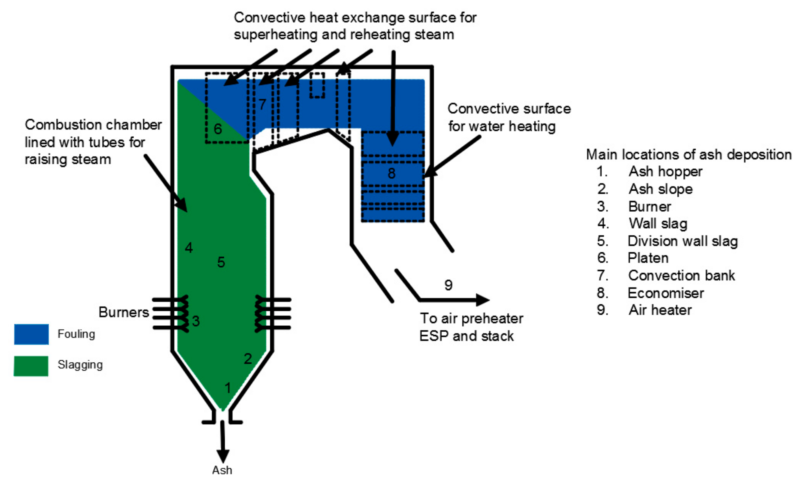
Deposit formation, erosion and corrosion are at the same time occurring issues that are regarding the quantity and composition of fuel mineral matter and frequently cause incorrect operation of the combustion system and boiler efficiency decrease. The ash agglomeration might limit the heat transfer and gas flow within the boiler and thus limit productivity and provide mechanical damages which may stop further boiler operation. Two types of deposit formation phenomena can be recognized: slagging and fouling. Slagging can be noticed within the high-temperature and refractory sections of the boiler like chamber walls or other surfaces that are located in the radiant section of the boiler. It appears as a result of radiative heat transfer, which is principally noted there and causes the occurrence of molten ashes. Slagging decreases the heat absorption in the chamber and then leads to growth in the furnace exit gas temperature. Whereas, fouling takes place in the furnace outlet and convective heat transfer sections of the boiler. Consequently, there are two forms of deposits. The first one is the high-temperature deposit (usually a result of slagging) which can appear where the flue gas temperature is in the range of 1300–900 °C. Slagging is accompanied by the generation of semi-fused and sintered ash deposits. The second is the low-temperature deposit which can generally be a result of fouling. This kind of deposit is related to the generation of powdery or gently sintered deposits. Fouling occurs in sections where the flue gas temperature is between 900–300 °C [9,10,11,12,13]. The position of these two kinds of deposition phenomena in the pulverized fuel boiler can be seen in Figure 1.

Biomass is a carbon-neutral fuel. Due to this, the exploitation of this kind of fuel brings several advantages. On the other hand, agglomeration, slagging and fouling or chlorine corrosion are technical issues that are associated during combustion or co-combustion of this type of fuel. For example, in comparison with conventional fuel combustion, a decrease in boiler efficiency can appear. The high content of alkali metals in biofuels (K and Na) can cause severe technical problems. In particular, the high potassium content is considered to be the most negative. Due to the presence of alkali metals in biomass, chlorine and silica, alkali silicate would be created with the presence of sulfur. These created compounds are represented by a low melting and softening point (

Table 1. Melting and eutectics points which occur during the combustion of biomass in power boilers [17].

Compound	Melting Temperature, °C	Eutectics	Eutectic Point, °C
ZnCl2	283	KCl-ZnCl2	230
PbCl2	489	NaCl-ZnCl2	262
FeCl2	673	KCl-FeCl2	355
ZnSO4	730	NaCl-FeCl2	370
KCl	775	K2SO4-ZnSO4-Na2SO4	388
NaCl	801	KCl-PbCl2	412
CrCl2	821	NaCl-PbCl2	415
Na2SO4	884	NaCl-CrCl2	437
NiCl2	1001	KCl-CrCl2	462
K2SO4	1076	KCl-NiCl2	508
CaSO4	1400	NaCl-NiCl2	560
PbSO4	1170	KCl-NaCl	657
ZnCl2	283	KCl-ZnCl2	230

). Because of this, the most serious and common problems that biomass boilers suffer from is rapid deposit formation (mainly slagging) on the surfaces of boiler heat exchangers [5,13,14,15,16].

Commonly, the ash deposition process can arise through four mechanisms: inertial impaction, condensation, thermophoresis, and chemical reactions [18,19]. The first of them (inertial impaction) occurs when particles are bigger than 10 μm. Because of adequate inertia, these particles follow the gas flow and during this, can hit the heat transfer surfaces by inertial forces. The second is the condensation process, which can appear when vapors pass across the cool surfaces. During this mechanism, they condense on already deposited particles or surfaces with a colder temperature in comparison to the gas flow. Next, the thermophoresis is related to the local temperature. This process takes place when particles are transported because local temperature gradients cause the movement of the particles. Finally, chemical reactions involve heterogeneous reactions between gas species and deposits. The most important chemical reactions which are connected with ash deposition are sulphation, oxidation, alkali absorption and generation of eutectics [11,18,19,20,21,22,23,24].

The combustion of biomass fuels, which came from the agricultural sector or contaminated waste materials intensify the ash-related trouble. There are some methods that have been found to reduce these problems that appear during biomass combustion, such as fuel mixing, the use of additives, and leaching out trouble elements [5,25,26,27,28]. One of these promising methods is using additives to reduce boilers problems [25,26,27,28,29,30,31,32]. In the literature, there are many descriptions connected to materials that have been inspected as reduction additives for boilers problems [25,26,27,28,31,32,33,34,35,36]. Mixing with fuel aluminosilicate additives such as halloysite may be an answer for biomass usage challenges.

The prediction of phase transformation of ashes from the combustion process is a topic often discussed by researchers around the world [37,38,39,40,41]. The estimation of the slagging ability of fuels is used in power boilers, waste incineration plants, and gasification installations. The excessive occurrence of hardly removable ash deposits reduces the heat exchange between steam and flue gases as a result, leading to a decrease in boiler efficiency. Deposit formation is also associated with corrosion and other technical problems. The easiest way to estimate the risk of slagging and fouling is to use the AFT test (Ash Fusion Temperature test) and learn about the deformation temperature or the softening temperature. Such models allow for estimating the behavior of ashes subjected to high-temperature processes based on the chemical composition of ash and/or fuel. The prediction of phase transformation of biomass ashes is challenging, due to the highly variable composition of these fuels, as well as the complex processes accompanying phase transformations [6]. Until now, a model with high reliability for biomass samples has not been developed. The existing models mainly use available databases, such as [37,42,43], with the chemical composition of ash samples combined with experimental results of phase transformations.

One of the first is the Seggiani model [37] successfully dedicated to predicting AFT (Ash Fusion Temperature) for ash from coal combustion. The model was built based on multiple regression, based on data containing 433 samples of coal ash and some biomass ash. This model calculates the characteristic temperatures of phase transitions: IDT—the temperature of initial deformation of ash, ST—softening temperature, HT—hemisphere temperature, FT—flow temperature and T_cv—critical viscosity temperature for coal ash samples. The model is characterized by temperature prediction with a standard error of less than 90 °C, using 49 independent variables.

The next one is a Holubcik model, also based on multiple regression to predict the characteristic melting temperatures of biomass ashes with additives [38]. However, in this model, a small population of N = 21 samples with nine independent variables was used, which may indicate the limited applicability of this model for a wider range of biomasses. The standard error of temperature estimation for the Holubcik model was below 70 °C.

For the prediction of phase transformations, models are also made based on neural networks, such as the Miao model [39]. This model predicts softening temperatures ST based on the chemical composition of 200 coal ash samples. In the best version, this model contains five variables and allows ST prediction with an average error not exceeding 3.59%.

Another author, Yang [40], based his nonlinear model on a database containing 77 samples of coal ashes. This model was built based on the SVM (Support Vector Machine) package from MATLAB^® software. This calculates the softening temperature ST for the tested samples with an accuracy of 86.7%.

Phase transition temperatures can also be determined based on thermodynamic equilibrium calculations, often using the FactSage^® software [41,44] for STA (Simultaneous Thermal Analysis) and equilibrium thermodynamic calculations to predict characteristic fusion temperatures [41]. The predicted temperature of ash sample deformation is near the designated temperature T₃₀ (30% of the mass of the sample occurs in the liquid phase). In the described tests, the results differ by less than 100 °C for straw and wood bark. By using the same model, the predicted temperatures of ash deformation from miscanthus and beech trees differed by less than 200 °C. Thus, it can be said that the model is sensitive to the type of biomass and the chemical composition of it.

The authors have not identified any other similar studies on the prediction of AFT (Ash Fusion Temperature) using the model dedicated to halloysite modified biomass. Additionally, the authors would like to point out the AFT model can be used as a productive tool in computational works which can be performed by engineers for raw and modified biomass. This model can also be used for necessary simulations in in the frame of the modern Industry 4.0 concept.

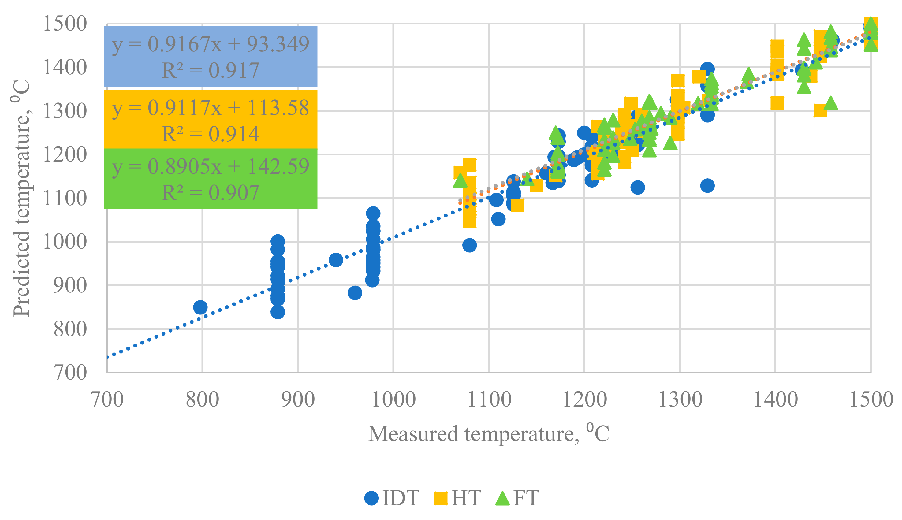
2. Ash Fusion Temperature Model

The AFT (Ash Fusion Temperature) model developed in this work was performed in Statistica 13.1. A software package containing statistical analysis using multiple progressive regression was used. This model is divided into three separate models, which are designed to predict the characteristic ash melting temperatures: IDT—initial deformation temperature, HT—hemisphere temperature, FT—flow temperature. It is based on the chemical composition of fuel and ash as is the standard [45]. IDT, HT, and FT temperatures are dependent variables in the discussed models. The model calculating shrink temperature SST was not made due to the incomplete database in this area. The regression model was made at the significance level of α = 0.05. For the discussed models (IDT, HT, FT), several coefficients describing multiple regression parameters are presented, such as the F—statistical significance level by Fisher–Snedecor test and p—corresponding probability level, R²—model determination coefficient, and S_e—standard error of estimation. The models are designed to predict AFT for biomass (raw and modified using fuel additive). Additionally, the co-authors used artificial neural networks to predict the same three biomass ash fusion temperatures. These results were presented separately in [46].

2.1. Fuel Database

To build the AFT model, a database describing 104 biomass samples of various types were taken from [47]. This paper provides information on the chemical composition of biomass samples as it collects data from available scientific references. Additionally, in the present study the fuel database was supplemented with experimental analyses carried out in the external laboratory. All of the analysis were performed in accordance with the official methodology that is established by the European Standard Technology Committee. Each sample is characterized by a complete data set (complete ash oxide analysis, AFT experiment results for IDT, HT, FT, sulfur and chlorine content in fuel). Incompletely analyzed samples were omitted.

Additionally, the database was extended by four samples of biomass which were tested during our own investigations (marked as BZ—herbaceous pellets, DM—miscanthus, DS—cereal straw, SPK—wheat straw). Four samples of biomass without additive (BZ0, DM0, DS0, SPK0) and four samples of biomass with the halloysite additive (BZ2, DM4, DS4, SPK4) were investigated (“0”—without halloysite, “2”—2 wt.% of halloysite, “4”—4 wt.% of halloysite).

Table 2. Results of proximate and ultimate analysis of investigated fuels.

	Proximate Analysis wt.% (As-Received State)
No.	BZ0	BZ2 *	DM0	DM4 *	DS0	DS4 *	SPK0	SPK4
Moisture	9.20	9.30	10.20	10.30	11.70	11.80	13.60	13.70
Ash	3.83	5.83	3.86	7.86	9.13	13.13	4.73	8.73
Volatiles	68.11	66.55	69.21	65.99	61.12	58.03	63.44	60.34
Fixed Carbon	18.86	18.32	16.73	15.85	18.05	17.04	18.22	17.23
	Ultimate Analysis wt.% (As-Received State)
C	43.34	42.34	43.34	41.67	38.98	37.01	39.69	37.75
H	5.38	5.25	5.38	5.17	4.85	4.60	5.03	4.78
S	0.09	0.09	0.09	0.09	0.11	0.11	0.08	0.07
N	2.68	2.62	2.68	2.58	0.76	0.72	0.47	0.76
Cl	0.08	0.08	0.08	0.07	0.38	0.36	0.15	0.38
Na	0.03	0.03	0.02	0.02	0.07	0.07	0.02	0.07
K	0.91	0.89	0.49	0.47	1.26	1.21	0.74	1.26
O	34.47	33.68	33.87	31.87	32.76	31.09	33.68	32.76
LCV (MJ/kg)	16.52	16.14	16.52	15.88	14.37	13.64	14.99	14.26

* Theoretical (calculated) fuel state is presented.

shows the analyses of used fuels. Proximate and ultimate analysis results for fuels without additive were carried out according to the international standards. In particular, proximate analysis was performed according to standards for biomass fuels, such as PN-ISO 18134, PN-EN-ISO 18122, PN-EN-ISO 18123. Ultimate analysis was carried out by the external laboratory by using a high-temperature combustion method with IR detection. The LCV was determined by the calorimetric method according to PN-EN 14918. Theoretical analyses for fuel-additive mixtures were performed from the individual as-received fuel analysis and the halloysite additive analysis results. Additionally, major oxide analysis (performed with the Thermo iCAP 6500 Duo ICP plasma spectrometer) and ash fusibility analysis (performed according to CEN/TS 15370-1:2007), for investigated fuels, are shown in

Table 3. Major oxide analysis of investigated ashes (as-received state).

Component/Fuel	BZ0	BZ2	DM0	DM4	DS0	DS4	SPK0	SPK4
SiO2, wt.%	46.17	46.06	62.54	53.61	56.46	54.93	62.46	53.55
Fe2O3, wt.%	2.07	7.86	0.77	8.82	1.87	3.91	0.85	8.58
Al2O3, wt.%	4.92	13.48	1.05	14.64	4.21	13.40	1.26	13.18
Mn3O4, wt.%	0.31	0.36	0.09	0.26	0.07	0.12	0.22	0.34
TiO2, wt.%	2.51	3.15	0.08	1.19	0.22	0.58	0.10	1.22
CaO, wt.%	15.69	10.46	9.54	6.66	9.76	7.60	7.66	5.35
MgO, wt.%	4.33	2.98	1.52	1.08	2.90	2.26	2.21	1.64
SO3, wt.%	4.11	2.71	2.56	1.36	2.22	1.50	2.48	1.64
P2O5, wt.%	4.46	3.20	4.52	3.38	2.84	2.38	3.35	2.62
Na2O, wt.%	1.03	0.82	0.33	0.32	0.97	0.84	0.32	0.25
K2O, wt.%	14.22	8.72	16.94	8.61	18.40	12.36	18.97	11.53
BaO, wt.%	0.13	0.15	0.03	0.05	0.05	0.07	0.08	0.09
SrO, wt.%	0.05	0.04	0.02	0.02	0.04	0.04	0.02	0.02

and

Table 4. Results of ash fusibility experiments of investigated fuels.

Oxidizing Conditions
Temp. °C/ Fuel	BZ0	BZ2	DM0	DM4	DS0	DS4	SPK0	SPK4
IDT	1100	1120	780	930	790	930	750	910
ST	1110	1230	940	1210	1080	1160	960	1200
HT	1130	1250	1170	1260	1150	1210	1070	1260
FT	1140	1260	1260	1270	1290	1260	1170	1280

.

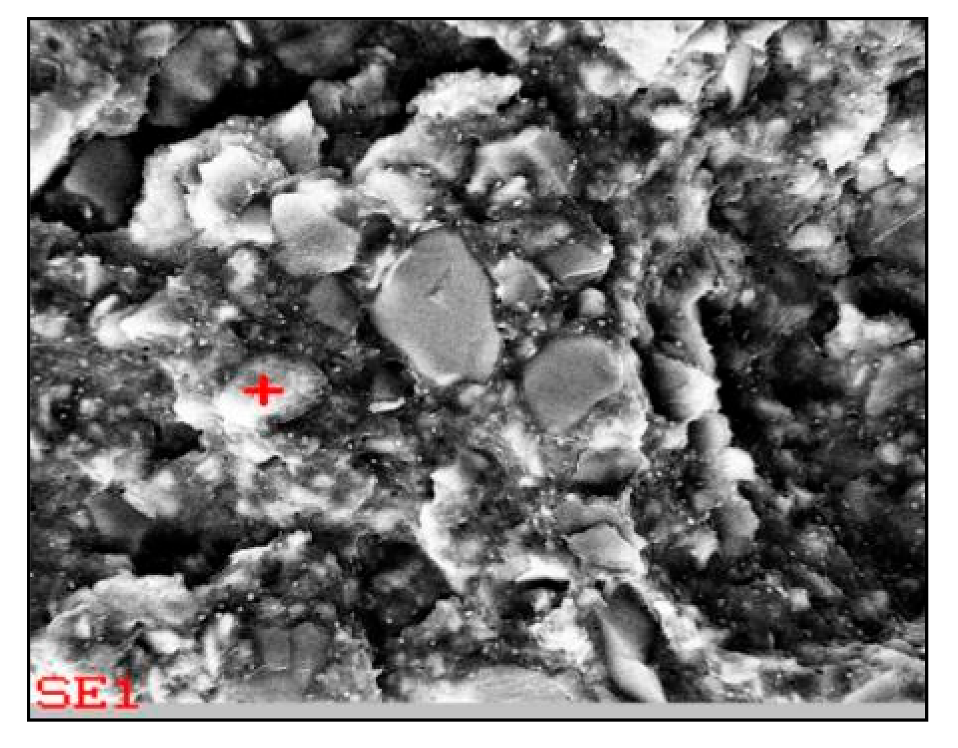
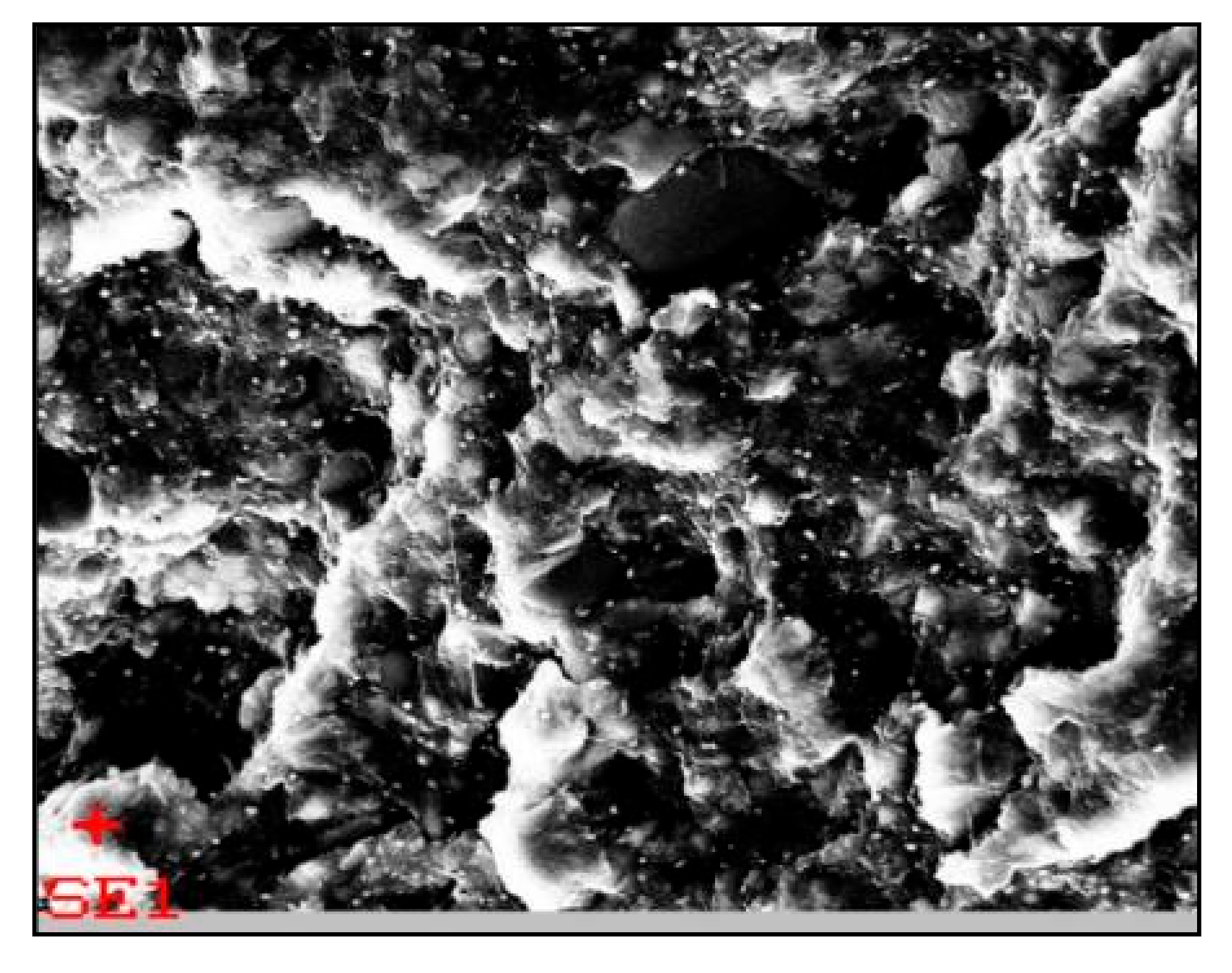
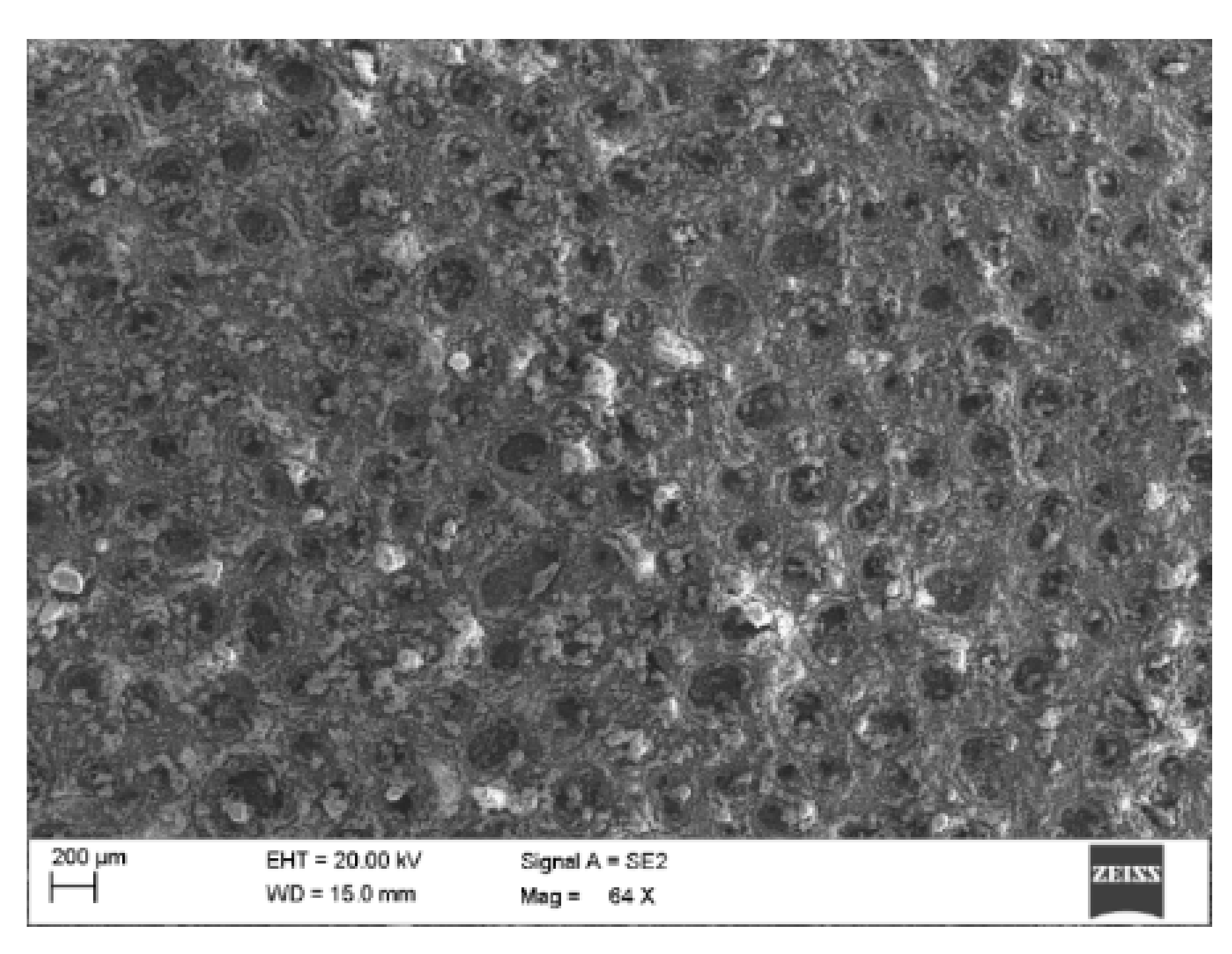
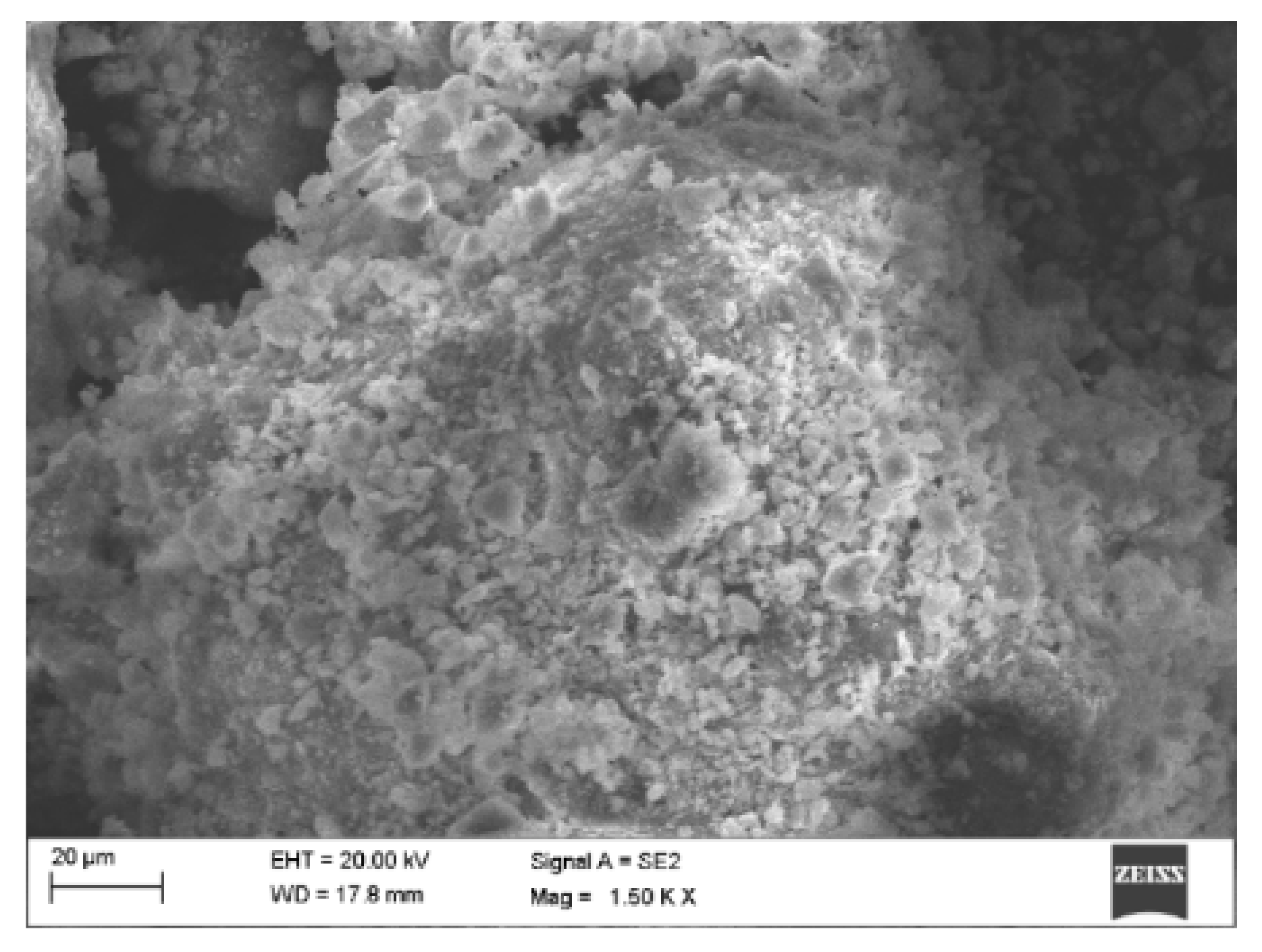
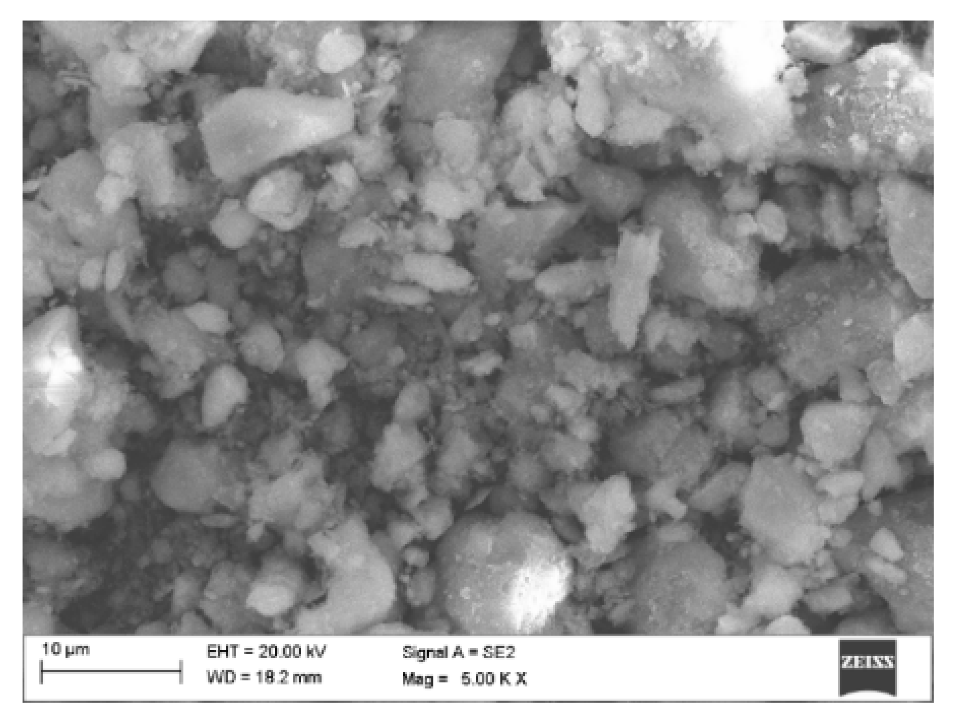
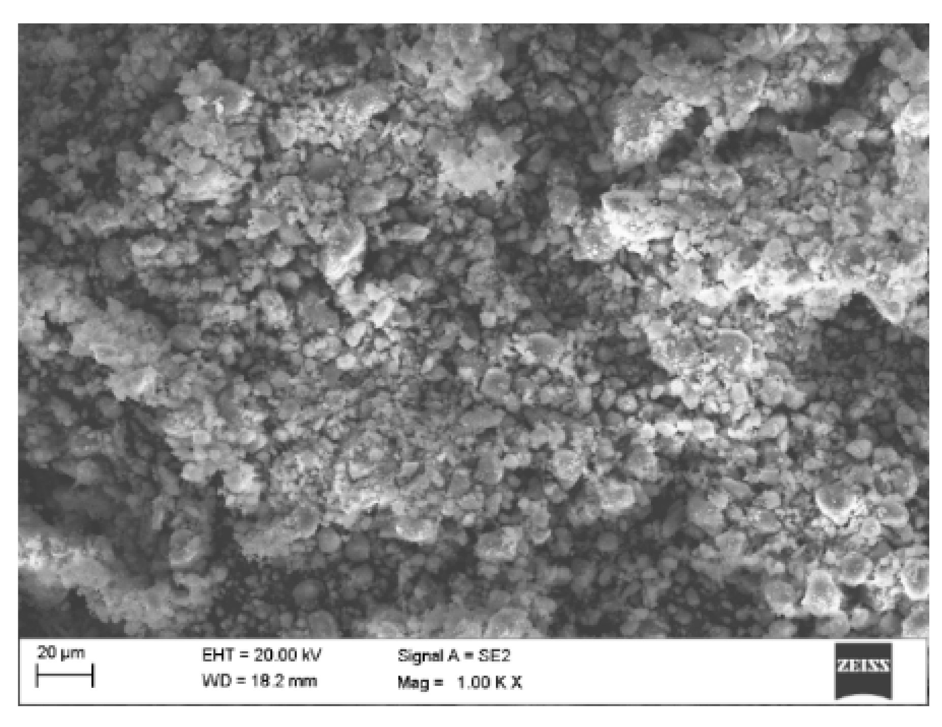
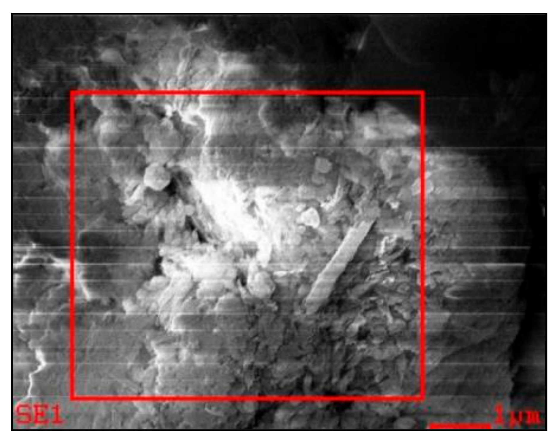
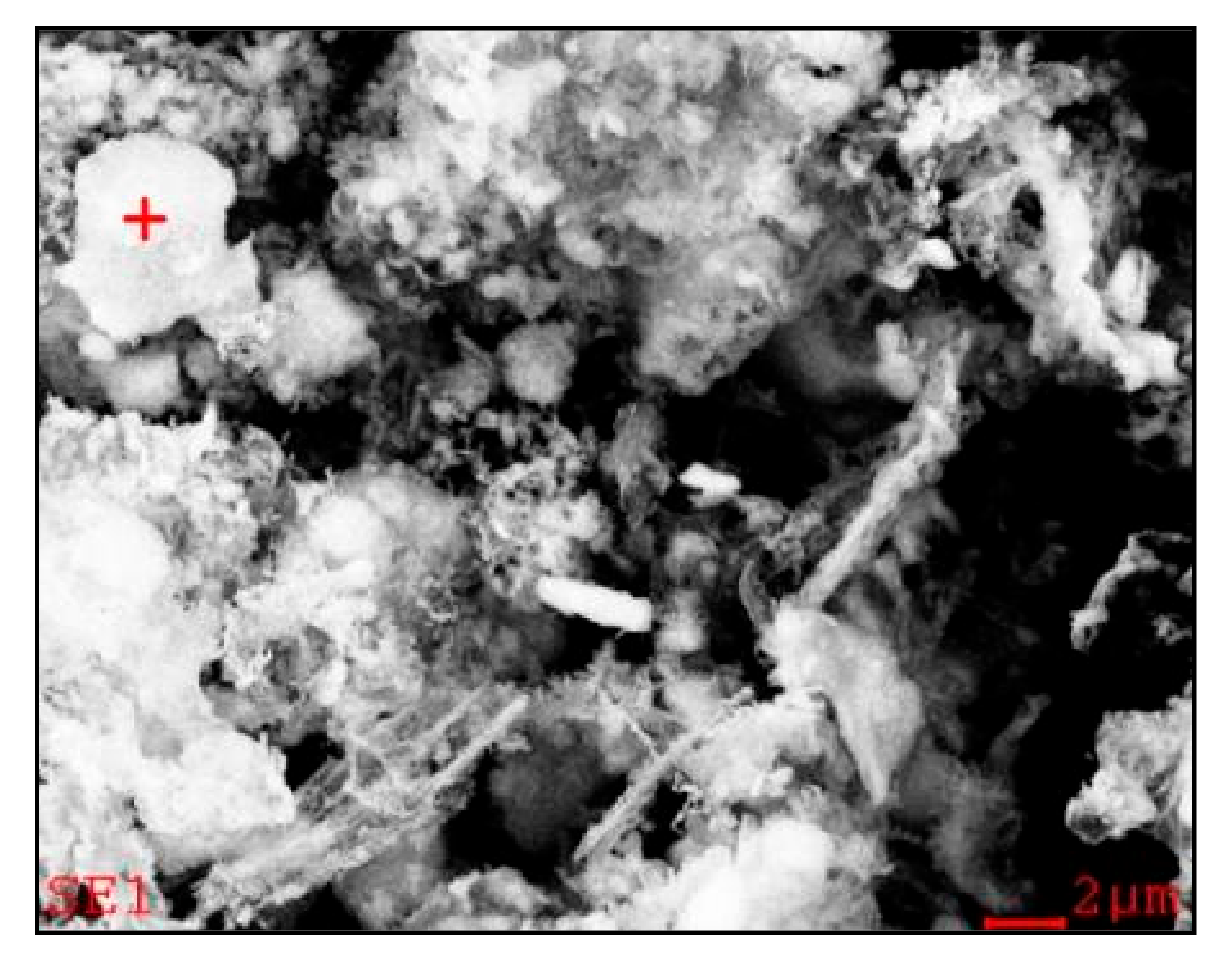
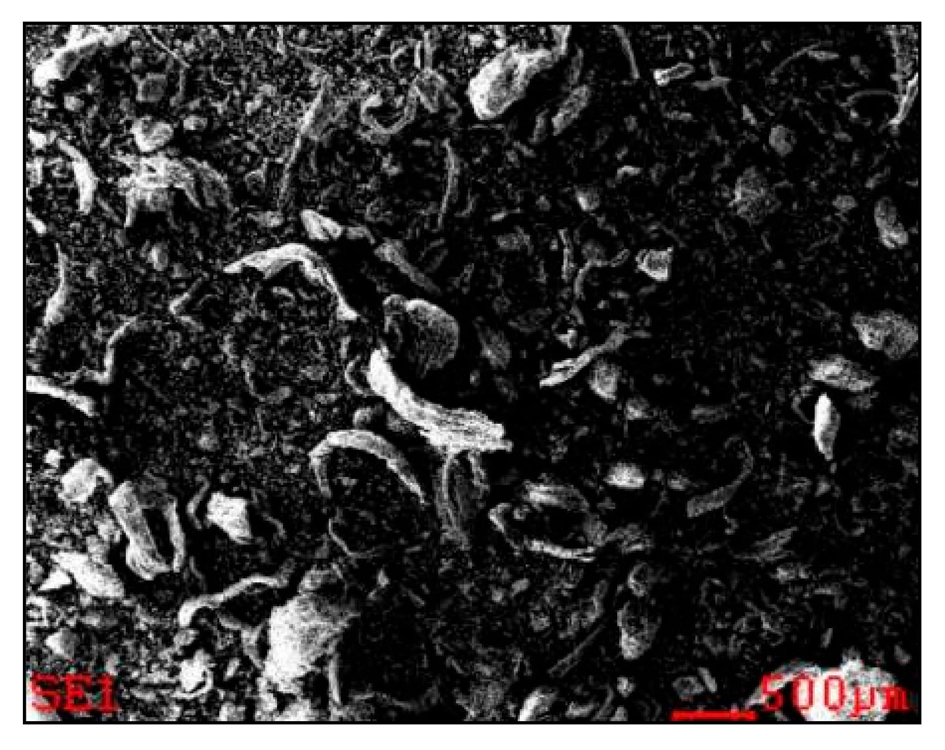
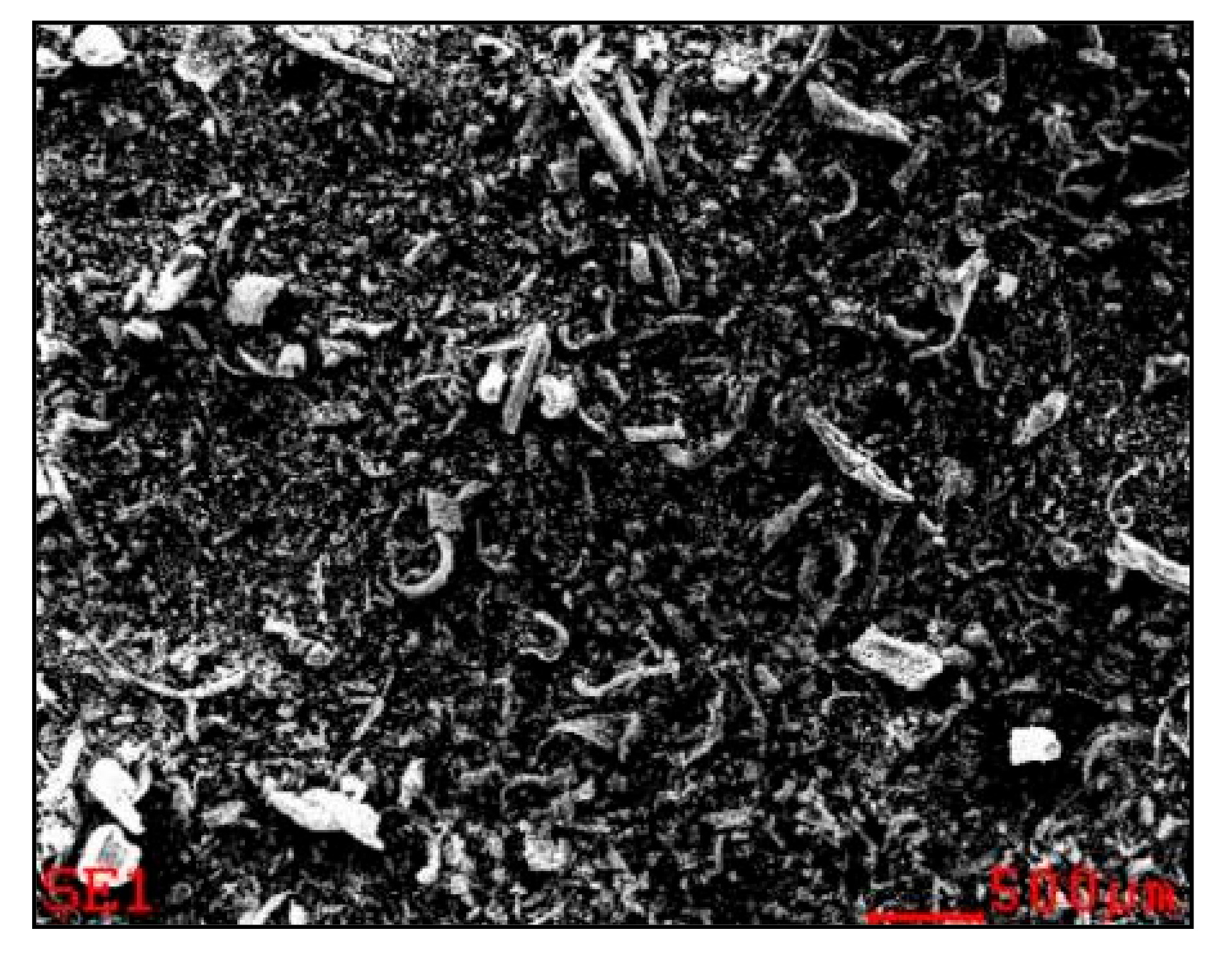
Moreover, morphological analyses of the structure of ash samples with and without halloysite were performed. Analytical samples with a particle size of <425 μm were prepared from the fuels specifically tested in this work. Initially, samples of biomass fuels were crushed to a fraction of <1000 μm in the LMN-240 knife mill, and then to a size <425 μm in the LMN-100 grinder. Mass doses of halloysite 2 wt.% or 4 wt.% were added to the biomass. The halloysite used in the research was characterized by a particle size of <350 μm and was added in an as-received state. The mixing of fuels with the addition of halloysite was carried out in a drum mixer. The sample homogenization time was 2 hours. Analytical biomass with and without additive was ashed at 550 °C. The samples prepared in this way were subjected to SEM-EDS microscopic analysis. The surface structure of the samples was tested in a Zeiss Supra 35 high-resolution scanning electron microscope, equipped with the Trident XM4 system by EDAX (EDS, WDS, EBSD) at a maximum accelerating voltage of 20 kV and magnification up to 50,000×. The qualitative and quantitative analysis of the chemical composition in the microareas of the tested sample surfaces was carried out with the use of EDS scattered X-ray energy detection. A structural examination of the sample surface was performed with the use of SE (secondary electron) imaging. The analysis included a raw sample of halloysite (HA-I–HA-VI), samples from biomass combustion without the addition of halloysite (BZ0, DM0, DS0, SPK0) and with the addition of halloysite (BZ2, DM4, DS4, SPK4). The results of the SEM-EDS analysis are presented later in this article.

Finally,

Table 5. Min and max—content of individual ash and fuel components.

Formula	Min	Max
SiO2 (wt.%)	0.00	94.48
CaO (wt.%)	0.97	72.39
K2O (wt.%)	0.23	63.90
P2O5 (wt.%)	0.00	40.94
Al2O3 (wt.%)	0.01	25.02
MgO (wt.%)	0.19	38.22
Fe2O3 (wt.%)	0.00	36.27
SO3 (wt.%)	0.36	45.89
Na2O (wt.%)	0.00	29.82
TiO2 (wt.%)	0.00	21.96
S d (wt.%)	0.01	2.33
Cl d (wt.%)	0.00	3.13

^d—dry state.

shows the min and max values of individual ash and fuel components entering the AFT model. The ranges of data entered are very wide—e.g., content of silica in the ash is in the range of 0.00–94.48 wt.%, potassium content: 0.23–63.90 wt.%, phosphorus content: 0.00–40.94 wt.%, sodium content 0.00–29.82 wt.%, sulfur content: 0.01–2.33 wt.%, chlorine content: 0.00–3.13 wt.%, etc. This demonstrates the potentially wide applicability of the AFT model for biomass with different chemical compositions, as well as for biomass with fuel additives.

2.2. Basics of Multiple Regression

The multiple regression is one of many ways to match a linear function to empirical data. The least-squares method is used in this regression, by means of which the regression line is selected that the sum of squares of the distance for measurement points from the regression line is as small as possible, this can be written as follows (1) [48]:

$${\displaystyle \sum }_{\mathrm{i}-1}^{\mathrm{n}}{({\mathrm{y}}_{\mathrm{i}}-{\hat{\mathrm{y}}}_{\mathrm{i}})}^2=\min$$

(1)

Through the application of this criterion, it is possible to choose practical structural parameters of the regression model β₀, β₁. The multiple regression model is described by Equation (2) [37,38]:

$$\mathrm{Y}={\mathsf{\beta }}_0+{\mathsf{\beta }}_1{\mathrm{X}}_1+{\mathsf{\beta }}_2{\mathrm{X}}_2+{\mathsf{\beta }}_{\mathrm{n}}{\mathrm{X}}_{\mathrm{n}}$$

(2)

where:

• $\mathrm{Y}$—dependent variable,
• ${\mathrm{X}}_1,{\mathrm{X}}_2,{\mathrm{X}}_{\mathrm{n}}$—independent variables,
• ${\mathsf{\beta }}_0,{\mathsf{\beta }}_1,{\mathsf{\beta }}_{\mathrm{n}}$—structural coefficients, assigned to successive independent variables.

There are several assumptions in the regression model. The model assumes the linearity of parameters and the stability of the relationship between the studied phenomena. Additionally, the random component is a random variable with a normal distribution N (0, σ2) [48]. To verify the fit of the model to the empirical data, the determination coefficient R² is most often used. R² is calculated from the following Equation (3) [49]:

$${\mathrm{R}}^2=\frac{{{\displaystyle \sum }}_{\mathrm{i}=1}^{\mathrm{n}}{\left({\hat{\mathrm{y}}}_{\mathrm{i}}-\overline{\mathrm{y}}\right)}^2}{{{\displaystyle \sum }}_{\mathrm{i}=1}^{\mathrm{n}}{\left({\mathrm{y}}_{\mathrm{i}}-\overline{\mathrm{y}}\right)}^2}$$

(3)

where:

• ${\hat{\mathrm{y}}}_{\mathrm{i}}$—the predicted value of the dependent variable;
• $\overline{\mathrm{y}}$—the average value of the dependent variable y.

The numerator of the above formula defines the variability of ${\hat{\mathrm{y}}}_{\mathrm{i}}$ and the predicted value, while the denominator checks the variability of the observed values of ${\mathrm{y}}_{\mathrm{i}}$. This means that the determination coefficient R² is a measure of matching the variable y to the predicted value. The R² coefficient takes values in the range of 0.0–1.0. The closer to 1.0, the better fit of the model to the empirical data. However, using only R² is not enough to assess the correctness of model prediction. A suitable parameter is the adjusted determination coefficient R²_adj (4). It evaluates the number of significant independent variables used in the model. The removal of irrelevant independent variables has the effect of increasing the R²_adj ratio [50]:

$${\mathrm{R}}_{\mathrm{adj}}^2{}^{}=1-\left(\frac{\left(1-{\mathrm{R}}^2\right)\left(\mathrm{n}-1\right)}{\mathrm{n}-\mathrm{m}-1}\right)$$

(4)

where:

• n—number of observations;
• m—number of independent variables in the model excluding the constant.

However, this coefficient always takes values lower than R². Another parameter describing the model fit to the empirical data is the standard error, also called the standard deviation of the residuals S_e. It is a very popular statistical parameter and determines the average difference between measured and predicted values. It is described by the following Equation (5) [51]:

$${\mathrm{S}}_{\mathrm{e}}^2=\frac{{{\displaystyle \sum }}_{\mathrm{i}=1}^{\mathrm{n}}{{\mathrm{e}}_{\mathrm{i}}}^2}{\mathrm{n}-\mathrm{k}-1}$$

(5)

where:

• n—number of observations;
• k—the average value of dependent variable y.

The next simple parameters verifying the correctness of model prediction include the absolute error Δx (6) and the relative error δ (7). These parameters are useful when analyzing specific prediction results.

$$\Delta \mathrm{x}=\left|\mathrm{x}-{\mathrm{x}}_0\right|$$

(6)

$$\mathsf{\delta }=\frac{\left|\mathrm{x}-{\mathrm{x}}_0\right|}{\mathrm{x}}·100\%$$

(7)

where:

• x—value from measurement;
• x₀—predicted value.

One of the basic methods of verifying the statistical significance of the multiple regression model is the use of the F-Fisher—Snedecor test [52]. It consists of checking whether there is a relationship between the dependent variable and the system of independent variables. The zero hypothesis H0 is tested for which the independent variables β_n are 0 (H0: β_n = 0) (hypothesis of no regression). An alternative is a hypothesis H1for which the regression coefficients reach values different from 0 (H1: ${\mathsf{\beta }}_{\mathrm{n}}$ ≠ 0), [53]. Next, the value of the F-Fischer–Snedecor test F_emp is calculated from Equation (8); the F_crit value is read from the Fisher–Snedecor test table and they are compared [52,53]. If F_emp > F_crit, then H0 must be rejected—the hypothesis of no regression. There is a linear regression relationship between the dependent variable and the independent variables system. If F_emp < F_crit, then H0 cannot be rejected. This would mean that the regression equation does not have a strong linear relationship. If the value of p (test probability) is lower than the adopted level of statistical significance, the structure of the model is correct and its assumptions are satisfied, the null hypothesis can be rejected. In the designated model, the H0 hypothesis is a hypothesis of no regression [54,55].

$${\mathrm{F}}_{\mathrm{emp}}=\frac{\frac{{\mathrm{S}}_{\mathrm{xy}}{}^2}{{\mathrm{SS}}_{\mathrm{y}}}·\left(\mathrm{n}-2\right)}{{\mathrm{SS}}_{\mathrm{y}}-\frac{{\mathrm{S}}_{\mathrm{xy}}{}^2}{{\mathrm{SS}}_{\mathrm{y}}}}$$

(8)

where:

• SS_x—the sum of squared deviations for the X (independent variable);
• SS_y—the sum of squared deviations for the Y (dependent variable);
• Sx_y—the sum of squared deviations for the X and Y characteristics (dependent and independent variable);
• n—the number of freedom degrees.

2.3. Indicators

Mathematical indicators that are more commonly used in the literature for the prediction of fuel slagging and fouling tendencies were compared. Despite the limitations related to these procedures, they are constantly used to estimate the tendency of biomass fuels to form deposits. Finally, the AFT model is based on several indicators selected from 103 tested independent variables. After all considerations and calculations, 42 independent variables were chosen for IDT and HT, and 40 for FT. The IDT, HT, FT indicators are presented in

Table 6. List of independent variables used in regression equations and structural parameters which were assigned to them for IDT, HT, and FT models [7,37,38,39,47,56].

IDT		HT		FT
N = 92	β	N = 92	β	N = 92	β
Constant	3209.07	Constant	153.64	Constant	2307.76
(SiO2 + Al2O3)∙K2O	−1.35	K2O∙SiO2	−0.17	Sr	1026.70
P2O5	−35.62	Fe2O3	158.02	(SiO2 + Al2O3) K2O	−0.16
B/A∙BAI	396.66	Na2O2	−0.67	Fe2O3	37.94
Na2O2	−0.66	SiO2∙CaO	0.11	P2O5	−8.00
2∙Sd/(K2O + Na2O)	−1295.60	P2O5	0.20	Na2O2	−0.46
Fu2	−0.01	CaO2	0.20	SiO2∙CaO	−0.10
B/A∙fph	0.33	B/A∙BAI	−32.31	CaO2	0.17
Fe2O3∙CaO∙K2O	−0.50	Al2O3	47.73	Dix	−6387.02
Fe2O3∙MgO	6.73	Dix	−9908.07	Fe2O3∙CaO	−1.94
R2502	−2993.99	(CaO + MgO)/Al2O3	1.68	Al2O32	−0.05
SiO2∙Fe2O3∙K2O	0.18	B/A∙Sr	−104.79	B/A∙BAI	42.30
SiO2/CaO	27.96	K2O2	−0.22	Fe2O3∙Al2O3	−0.09
Cld∙Rs	9.72	MgO2	0.02	Fe2O3∙MgO	6.19
B/A∙Fu	0.40	B/A∙fph	−1.09	MgO	−43.39
Dr	−1785.53	Fe2O3∙CaO	−1.68	SV	−2934.82
Fu	−2.46	B/A∙Dix	406.96	B/A∙Sr	−87.46
B/A∙Sr	102.05	Na2O∙(B/A)	−3.96	B/A∙Dix	375.20
CaO+MgO	−53.80	SO3	75.32	Na2O∙(B/A)	−2.04
SV2	7604.73	Na2O	20.82	SO3	39.85
SiO2∙Rs	0.10	Fu2	0.00	TiO22	−1.26
(SiO2 + P2O5 + K2O)/(CaO + MgO)	−28.57	B/A	3.81	TiO2	−94.82
B	39.65	B/A∙Fu	−0.01	CaO	−13.46
B/A∙Dix	293.00	Fe2O3∙MgO	1.50	(CaO + MgO)/Al2O3	1.81
Al2O3∙CaO∙K2O	0.12	CaO∙MgO	−0.26	Al2O3∙CaO	0.02
B/A∙fcmk	0.00	K2O∙MgO	0.30	CaO∙MgO∙K2O	0.02
Na2O∙(B/A)	−1.23	Cld∙Rs	19.62	(Al2O3 + SiO2)/(Na2O + K2O)	−5.65
BAI∙Fu	−11.37	K2O∙BAI	−51.85	SiO2∙Fe2O3	0.32
SiO2∙CaO∙K2O	0.06	Fe2O3∙Al2O3	−2.06	SV2	1340.11
SV	−7785.94	K2O∙Fe2O3	−1.57	fph	−18.00
exp(10−2∙SiO2∙Al2O3)	0.00	K2O	31.22	K2O∙TiO2	4.93
Fe2O3/CaO	−429.15	SiO22	0.40	Fu	0.37
TiO2	−4.89	SV	−615.34	K2O∙SO3	−0.23
Dr2	3363.29	Fe2O32	−1.27	Cld 2	7.54
Al2O3 + SiO2/(Na2O + K2O)	−16.84	Al2O3 + SiO2/(Na2O + K2O)	−14.49	P2O52	−0.34
Cld	40.41	Dr2	693.36	K2O∙BAI	−24.06
P2O52	−0.26	Al2O3∙CaO	−0.21	Fe2O3∙Al2O3	−1.41
exp(10−4∙SiO2∙Al2O3)	−2071.35	Sd 2	−124.35	Fe2O32	−1.21
R250	4298.52	Sr	1015.75	K2O∙P2O5	0.33
Al2O3∙CaO	−1.41	fph	7.61	MgO2	0.30
abs(B/A-1)	−80.32	SV2	857.03	K2O∙CaO	−0.26
MgO2	−0.43	2Sd/(K2O + Na2O)	492.90
Al2O3	40.42	SiO2 + Al2O3	−33.15

. Independent variables that have a significant statistical impact (for which the probability of test statistics reached p < 0.05) are marked in red.

Below, there are indicators that have more complex equations which cannot be included in the Equations (9)–(20). They were obtained from the literature [7,37,38,39,47,56]:

$${\mathrm{D}}_{\mathrm{r}}=\frac{\mathrm{CaO}+\mathrm{MgO}}{{\mathrm{SiO}}_2+\mathrm{CaO}+{\mathrm{K}}_2\mathrm{O}+\mathrm{MgO}+{\mathrm{Al}}_2{\mathrm{O}}_3}$$

(9)

$${\mathrm{D}}_{\mathrm{ix}}=\frac{{\mathrm{SO}}_3+{\mathrm{S}}^{\mathrm{d}}}{{\mathrm{S}}^{\mathrm{d}}+{\mathrm{SO}}_3+{\mathrm{Fe}}_2{\mathrm{O}}_3+100}$$

(10)

$${\mathrm{f}}_{\mathrm{ph}}=\frac{\mathrm{CaO}+\mathrm{MgO}+{\mathrm{K}}_2\mathrm{O}}{{\mathrm{SiO}}_2+{\mathrm{Al}}_2{\mathrm{O}}_3}$$

(11)

$${\mathrm{f}}_{\mathrm{CMK}}=\frac{\mathrm{CaO}+\mathrm{MgO}}{{\mathrm{K}}_2\mathrm{O}}$$

(12)

$$\mathrm{SV}=\frac{{\mathrm{SiO}}_2}{{\mathrm{SiO}}_2+{\mathrm{Fe}}_2{\mathrm{O}}_3+\mathrm{CaO}+{\mathrm{K}}_2\mathrm{O}+\mathrm{MgO}}$$

(13)

$$\mathrm{R}250=\frac{{\mathrm{SiO}}_2+{\mathrm{Al}}_2{\mathrm{O}}_3}{{\mathrm{SiO}}_2+{\mathrm{Al}}_2{\mathrm{O}}_3+{\mathrm{Fe}}_2{\mathrm{O}}_3+\mathrm{CaO}}$$

(14)

$$\mathrm{B}={\mathrm{Fe}}_2{\mathrm{O}}_3+\mathrm{CaO}+\mathrm{MgO}+{\mathrm{Na}}_2\mathrm{O}+{\mathrm{K}}_2\mathrm{O}+{\mathrm{P}}_2\mathrm{O}$$

(15)

$$\mathrm{A}={\mathrm{SiO}}_2+{\mathrm{Al}}_2{\mathrm{O}}_3+{\mathrm{TiO}}_2$$

(16)

$$\mathrm{BAI}=\frac{{\mathrm{Fe}}_2{\mathrm{O}}_3}{{\mathrm{Na}}_2\mathrm{O}+{\mathrm{K}}_2\mathrm{O}}$$

(17)

$$\mathrm{Rs}=\frac{\mathrm{B}}{\mathrm{A}}·{\mathrm{S}}^{\mathrm{d}}$$

(18)

$$\mathrm{Fu}=\frac{\mathrm{B}}{\mathrm{A}}·\left({\mathrm{Na}}_2\mathrm{O}+{\mathrm{K}}_2\mathrm{O}\right)$$

(19)

$$\mathrm{Sr}=\frac{{\mathrm{SiO}}_2·100}{{\mathrm{SiO}}_2+{\mathrm{Fe}}_2{\mathrm{O}}_3+\mathrm{CaO}+\mathrm{MgO}}$$

(20)

2.4. Model Limitations

To calculate IDT, HT, FT temperatures, complete oxide composition should be given and normalized to 100 wt.% (SiO₂ + CaO + K₂O + P₂O₅ + Al2O₃ + MgO + Fe₂O₃ + SO₃ + Na₂O + TiO₂ = 100 wt.%), as well as the sulfur content in the fuel in dry state S^d (wt.%) and chlorine content in dry fuel in dry state Cl^d (wt.%). Below, the assumptions for model limits were described.

• The analytical biomass sample should be fired in a muffle furnace at 550 °C in accordance with PN-EN ISO 18122: 2016-01 [57];
• Oxide analysis of the ash sample must be in accordance with the procedure described in [58] and normalized to 100 wt.%;
• The content of individual ash components must be kept in the min/max range, which is given in Table 5;
• Analysis of sulfur and chlorine content in the fuel must be in accordance with the procedure described in [59] and given in wt.% of the dry matter content;
• The model calculates the characteristic fusion temperatures (IDT, HT, FT) of the ash sample under the oxidation atmosphere in the temperature range 700 °C ≤ x ≤1500 °C (AFT experiment range [45]); results outside should be rejected as unreliable.

3. Results and Discussion

3.1. Fuel Database—Morphological Analyses of the Structure for Ash Samples

Microscopic photos in various scales of 1, 2, 5, 10, 20, 100, 200, 500 μm depending on the size of the tested material particles were taken and subjected to EDS analysis. Morphological studies of the halloysite sample (six different photos were taken: HA-I÷HA-VI) indicate that the tested additive takes the form of oval grains rather than platelets and nanotubes. Photos of the halloysite sample are shown in Figure 2, Figure 3, Figure 4, Figure 5, Figure 6 and Figure 7. Further on, Figure 8, Figure 9, Figure 10 and Figure 11 present selected photos of DS4 and SPK4 samples on the 1 and 2 μm scale (with the addition of halloysite).

In Figure 8, an area with a high content of halloysite particles was identified. On the other hand, in Figure 9, the halloysite particle present in the ash of the SPK4 sample was marked in points. The following photos (Figure 10 and Figure 11) show images of DS4 and SPK4 samples in the 500 μm scale. Based on the microscopic examination alone, it cannot be clearly defined whether the selected ash grain is a halloysite particle. Only using EDS analysis, it is possible to determine the mass elemental composition of the studied area. Thanks to which, knowing the appropriate ratios of elements in the raw particle of halloysite and the reaction products with its participation, it can be identified and the sorption capacity of halloysite can be determined; for instance in the case of alkali metals (K and Na) or heavy metals.

Table 7. SEM-EDS analysis results for raw halloysite samples (HA-I÷HA-VI).

No. Samples	HA-I	HA-II	HA-III	HA-IV	HA-V	HA-VI
Photo Scale, μm	5	5	1	10	1	1
Scanned Area	Point	Point	Surface	Surface	Surface	Surface
OK	35.92	37.53	41.80	42.57	41.17	40.28
MgK	0.00	0.00	0.00	0.00	0.00	0.00
AlK	26.86	25.93	19.66	20.37	20.12	20.41
SiK	33.95	30.93	24.99	25.60	25.70	26.65
PK	0.00	0.00	0.00	0.00	0.00	0.00
SK	0.00	0.00	0.00	0.00	0.00	0.00
ClK	0.00	0.00	0.00	0.00	0.00	0.00
KK	0.00	0.00	0.00	0.00	0.00	0.00
CaK	0.00	0.00	0.00	0.00	0.00	0.00
FeK	3.26	5.61	11.68	9.83	11.31	11.26
TiK	0.00	0.00	1.87	1.62	1.71	1.41
NaK	0.00	0.00	0.00	0.00	0.00	0.00
Al/Si	0.79	0.84	0.79	0.80	0.78	0.77

,

Table 8. SEM-EDS analysis results for samples which were ashed at 550 °C (SPK0, SPK4, DS0, DS4).

No. Samples	SPK0-I	SPK4-I	SPK4-II	DS0-I	DS4-I	DS4-II
Photo Scale, μm	500	500	2	200	500	1
Scanned Area	Surface	Surface	Point	Surface	Surface	Surface
OK	32.33	37.87	35.74	36.40	35.08	37.31
MgK	1.90	1.70	0.82	1.89	1.80	0.97
AlK	1.93	6.90	21.04	1.88	5.66	16.35
SiK	24.13	26.40	26.73	26.26	25.84	21.67
PK	1.94	1.67	0.49	2.60	1.61	0.00
SK	0.97	1.03	0.00	1.29	0.86	0.00
ClK	1.38	1.21	0.00	1.40	1.54	2.07
KK	16.10	11.26	13.18	14.57	13.54	17.49
CaK	8.96	6.59	0.00	10.48	9.11	1.30
FeK	1.91	4.81	1.99	2.87	4.54	2.04
TiK	0.00	0.85	0.00	0.00	0.00	0.00
NaK	21.12	0.00	0.00	0.00	0.00	0.80
Al/Si	0.08	0.26	0.79	0.07	0.22	0.75

and

Table 9. SEM-EDS analysis results for samples which were ashed at 550 °C (DM0, DM4, BZ0, BZ2).

No. Samples	DM0-I	DM4-I	DM4-II	DM4-III	BZ0-I	BZ2-I	BZ2-II
Photo Scale, μm	200	500	10	20	200	500	2
Scanned Area	Surface	Surface	Point	Point	Surface	Surface	Point
OK	39.89	39.86	23.70	37.64	38.05	34.60	38.90
MgK	3.46	0.91	0.46	-	4.24	4.60	6.25
AlK	0.71	7.18	10.89	23.95	0.96	5.05	10.78
SiK	17.25	28.15	15.38	29.25	16.17	10.43	12.79
PK	2.89	1.91	1.38	0.00	2.73	2.83	2.77
SK	1.65	1.17	0.78	0.00	1.78	2.33	1.62
ClK	1.06	0.51	0.00	0.00	1.63	1.07	0.95
KK	17.18	8.53	8.43	4.76	18.59	15.92	13.28
CaK	15.56	6.88	1.68	0.00	15.17	17.80	10.59
FeK	0.00	5.07	35.23	2.35	0.00	4.09	2.08
TiK	0.00	0.00	2.08	2.05	0.00	0.91	0.00
NaK	0.00	0.00	0.00	0.00	0.00	0.00	0.00
Al/Si	0.09	0.26	0.71	0.82	0.08	0.48	0.84

presents the results of the EDS analysis of the tested samples.

Untreated halloysite samples are characterized by the Al/Si ratio in the range of 0.79–0.84 (Table 7). The tested samples showed the content of Fe in the range of 9.83 wt.%–11.68 wt.%, and Ti 1.41 wt.%–1.87 wt.% for the surface tests. On the other hand, based on the chemical formula and the molar mass of the two basic reaction products of halloysite with KCl—i.e., kalsilite (KAlSiO₄) and leucite (KAlSi₂O₆)—for which the Al/Si ratios are 0.96 and 0.48, respectively, an attempt can be made to identify the compounds formed with some degree of probability. Nevertheless, there is also a possibility of misidentification of a molecule with a similar Al/Si ratio and derived from other compounds present in biomass ash, such as anorthite (CaAl₂Si₃O₈), gehlenite Ca₂FeAlSiO₇, gismondite (Ca₂Al₄Si₄O₁₆ · 9H₂O), metakaolinite (Al₂Si₂O₅), Na–melilite (NaCaAlSi₂O₇) [6,7].

By analyzing the results in Table 8, for the SPK0-I sample (scanned surface), the Al/Si ratio was 0.08. However, for the SPK4-I sample (scanned area) it was 0.26. The increase in the Al/Si ratio is due to the presence of halloysite in the sample. This growth trend is maintained for all other DS4, BZ2 and DM4 samples compared to the samples without halloysite (DS0, BZ0, DM0). Changes in the shares of individual elements for enriched ashes result from the dosing of halloysite to the fuel. It is particularly important to determine the chlorine content in samples with and without halloysite using EDS. Table 8 and Table 9 show the results of point samples (SPK4-II, DM4-II, DM4-III) which were identified as molecules of reaction products with halloysite for which the Al/Si ratio is in the range 0.96–0.48. No chlorine was found in these samples. On the other hand, for the image of the sample area for the 1 μm scale (marked as DS4-II Figure 8) a significant Cl content was identified at the level of 2.07 wt.% (higher than for the 500 μm area—DS4-I, amounting to 1.54 wt.% and also higher than for samples without halloysite DS0-I—1.40 wt.%). It can be concluded that the reaction of halloysite with KCl was not completed, meaning that unreacted KCl, KCaCl₃ or the chlorine content may come from CaCl or NaCl, which were included in the scan area. Analyzing the chlorine content from photo BZ2-II (point) from Table 9, which is 0.95 wt.% with a significant Ca content of 10.59 wt.% and K equal to 13.28 wt.%, and in the absence of Na, the presence of chlorine may be caused by KCl, KCaCl₃ or CaCl.

It should also be noted that the results of the EDS analysis were normalized to 100 wt.% of the mass, eliminating the determined carbon content from the carbon strip, which is used as a base for the ash sample. Moreover, the presence of additional amounts of carbon element resulting from possible unburnt carbon presence in the ash sample cannot be completely excluded.

3.2. AFT Model

The prediction of characteristic ash fusibility temperatures is a complicated issue due to the complex processes occurring during combustion and the interaction of ash components between them. It is possible to predict the phase transitions of ash from biomass, based on its chemical composition, but only with a certain approximation.

Table 10. Summary of AFT regression results for temperatures: IDT, HT, and FT.

IDT		HT		FT
R multiple	0.952	R multiple	0.952	R multiple	0.947
R2 multiple	0.907	R2 multiple	0.906	R2 multiple	0.897
${\mathrm{R}}_{\mathrm{adj}}^2$	0.825	${\mathrm{R}}_{\mathrm{adj}}^2$	0.825	${\mathrm{R}}_{\mathrm{adj}}^2$	0.816
Femp (42.49)	11.12	Femp (42.49)	11.20	Femp (40.51)	11.10
p	4.98 × 10−14	p	2.68 × 10−14	p	1.74 × 10−14
Se	70.05	Se	51.98	Se	47.52

shows the results for three separate models—IDT, HT, and FT—which were prepared for the fuel database. For all models, the value of the statistics made with the Fisher–Snedecor F_emp test is in the range of 11.10–10.20 above F_crit with probability levels p < 0.05. Obtained R² determination coefficients for IDT, HT, and FT are 0.907, 0.906, and 0.897, which means that the variability of the model-dependent variables were explained in 90.7% for IDT; 90.6% for HT, 89.7% for FT.

In turn, the R²_adj parameter was obtained at the level of 0.825 for IDT and HT and 0.816 for FT, which describes the influence of significant independent variables used in the model on the obtained results of characteristic ash fusibility temperatures. Predicted temperatures IDT, HT and FT are characterized by the following standard estimation errors: 70.05; 51.98; 47.52. One can conclude that the use of the AFT model allows for the prediction of the temperature with an average error of <±70.05 °C for IDT; <±51.98 °C for HT; <±47.52 °C for FT. The results of the IDT, HT and FT models (which were presented in Table 10) describe the models with results which are out of the scope of the AFT experiment (700 °C ≤ x ≤ 1500 °C). For models of IDT, HT, FT respectively, 12, 11 and 13 prediction results were out of range. Prediction results of characteristic fusion temperatures are shown in Figure 12, where on the abscissa there are results from the experiment and, on the ordinate, there are results of the predicted temperature using the model. After the removal of predicted values outside the experimental range AFT 700 °C ≤ x ≤ 1500 °C, the determination coefficient R² for IDT, HT and FT was 91.7%; 91.4%; 90.7%. Then, the standard error of estimation S_e was determined, which for IDT, HT, and FT were, respectively, 48.62, 37.15, and 34.02 °C.

The AFT model is characterized by a more accurate adjustment to empirical data (high coefficient of determination) and small standard estimation error compared to literature models [37,38,39,40,41]. The negative features of the model include a small number of observations (N = 92) on which the model was created with a large number of independent variables 40–42. This is mainly due to difficulties in finding complete databases for biomass.

For the biomass studied in this paper, the results of the temperatures of ash phase transitions as well as their predicted values using the AFT model were presented in

Table 11. Measured and predicted AFT temperatures for biomass without and with the addition of halloysite.

	IDT				HT				FT
Sample	Observed Value (°C)	Predicted Value (°C)	Δx (°C)	δ (%)	Observed Value (°C)	Predicted Value (°C)	Δx	δ (%)	Observed Value (°C)	Predicted Value (°C)	Δx (°C)	δ (%)
BZ0	1110	1051.40	58.6	5.28	1130	1083.80	46.2	4.09	1140	1144.03	4.0	0.35
BZ2	1230	1204.67	25.3	2.06	1250	1209.26	40.7	3.26	1260	1140.75	70.7	6.61
DM0	940	958.11	18.1	1.93	1170	1151.83	18.2	1.55	1260	1258.68	1.3	0.10
DM4	1210	1214.55	4.6	0.38	1260	1252.65	7.4	0.58	1270	1259.96	10.0	0.79
DS0	1080	991.54	88.5	8.19	1150	1128.97	21.0	1.83	1290	1226.38	63.6	4.93
DS4	1160	1156.90	3.1	0.27	1210	1202.70	7.3	0.60	1260	1277.12	17.1	1.36
SPK0	960	882.58	77.4	8.06	1070	1158.44	88.4	8.27	1170	1249.88	79.9	6.83
SPK4	1200	1249.10	49.1	4.09	1260	1290.66	30.7	2.43	1280	1294.52	14.5	1.13

. In some cases—e.g., DS0 and SPK0 with IDT prediction—quite significant absolute errors of 88.5 °C and 77.4 °C were obtained. They are higher than the average difference between the measured temperature and the designated model (Se(IDT) = 70.05 °C). For the predicted HT temperature, SPK0 also exceeds the standard error of 51.98 °C. For the last projected HT temperature, values greater than the average difference between S_e values were determined for DS0, SPK0, and BZ2.

4. Summary

This article describes morphological analyses of the structure of ash samples and the statistical model of AFT prediction for characteristic ash melting temperatures from biomass using multiple regression. The possibility of predicting the phase transformation of ash based on its chemical composition as well as the content of sulfur and chlorine in the fuel was shown. The model can also be used for biomass with modified composition using additives.

Based on the obtained results, particular conclusions can be made:

• According to SEM-EDS results, halloysite samples are characterized by the Al/Si ratio in the range of 0.79–0.84 (Table 7). The tested samples also showed the content of Fe in the range of 9.83 wt.%–11.68 wt.%, and Ti 1.41 wt.%–1.87 wt.% for the surface tests;
• The increase in the Al/Si ratio in biomass samples is due to the presence of halloysite. This growth trend is maintained for all other DS4, BZ2 and DM4 samples compared to the samples without halloysite (DS0, BZ0, DM0);
• To fully identify the individual compounds present in the ash, it would be necessary to additionally perform X-Ray Diffraction analysis;
• Despite the existence of a large number of indicators that are used to predict the slagging and fouling tendencies of fuels, only a few have a significant statistical impact as independent variables used in the regression equations to determine IDT, HT, FT temperatures (42 independent variables for IDT and HT, and 40 for FT) (Table 6);
• The presented AFT model has some limitations (see Section 2.4);
• It is possible to predict the phase transitions of ash from biomass based on its chemical composition, but only with a certain approximation;
• R² adjustments for empirical data for ID, HT, and FT models were obtained, respectively, at the level of 90.7%; 90.6%; 89.7%;
• The use of the AFT model allows for the prediction of the temperature with an average error of <±70.05 °C for IDT; <±51.98 °C for HT; <±47.52 °C for FT;
• Removal of predicted values outside the experimental range AFT 700 °C ≤ x ≤ 1500 °C allows for achieving the determination coefficient R² for IDT, HT and FT at the levels of 91.7%; 91.4%; 90.7% (S_e below 50 °C)—IDT: S_e < 48.62 °C; HT: S_e < 37.15 °C; FT: S_e < 34.02 °C;
• For some of the additionally tested biomass, a higher than the average difference between the measured temperature and the designated model was observed (IDT: BZ0—58.6 °C, DS0—88.5 °C, SPK0—77.4 °C, SPK4—49.1 °C; HT: BZ0—46.2 °C, BZ2—40.7 °C, SPK0—88.4 °C; FT: BZ2—70.7 °C, DS0—63.6 °C, SPK0—79.9 °C);
• Absolute error Δx for all additionally tested biomass was lower than 90.0 °C;
• The AFT model discussed in this article is suitable for predicting ash fusion temperatures for biomass (raw and modified using fuel additive);
• The AFT model can be used as an effective tool in some computational works or for predictive simulations in diverse energetic applications of biomass required by the modern Industry 4.0 strategy. Additionally, it can be used as a laboratory test substitute to predict characteristic ash melting temperatures, which can save money and time for heat and power engineers;
• To make the AFT model generally applicable, additional tests and validations for different biomass fuels and ash fractions are recommended as the chemistry involved in the ash melting process may vary from case to case and, therefore, a careful and comprehensive stepwise validation is needed.

References

1. Van Loo, S.; Koppejan, S. The Handbook of Biomass Combustion and Co-Firing; Earthscan: London, UK, 2010. [Google Scholar]
2. Pronobis, M. Evaluation of the influence of biomass co-combustion on boiler furnace slagging by means of fusibility correlations. Biomass Bioenergy 2005, 28, 375–383. [Google Scholar] [CrossRef]
3. Kleinhans, U.; Wieland, C.; Frandsen, F.J.; Spliethoff, H. Ash formation and deposits in coal and biomass fired combustion systems: Progress and challenges in the field of ash particle sticking and rebound behavior. Prog. Energy Combust. Sci. 2018, 68, 65–168. [Google Scholar] [CrossRef]
4. Liao, Y.; Wu, S.; Chen, T. The alkali metal characteristic during biomass combustion with additives. Energy Procedia 2015, 75, 124–129. [Google Scholar] [CrossRef] [Green Version]
5. Wang, L.; Hustad, J.E.; Skreiberg, O.; Skjevrak, G.; Gronli, M. A critical review on additives to reduce ash related operation problems in biomass combustion applications. Energy Procedia 2012, 20, 20–29. [Google Scholar] [CrossRef] [Green Version]
6. Vassilev, S.V.; Baxter, D.; Vassileva, C.G. An overview of the behaviour of biomass during combustion: Part II. Ash fusion and ash formation mechanisms of biomass types. Fuel 2014, 117, 152–183. [Google Scholar] [CrossRef]
7. Vasilev, S.; Baxter, D.; Andersen, L.K.; Vasileva, C.K. An overview of the composition and application of biomass ash. Part 1. Phase–mineral and chemical composition and classification. Fuel 2013, 105, 40–76. [Google Scholar] [CrossRef]
8. Pronobis, M. Modernizacja Kotłów Energetycznych; WNT: Warszawa, Poland, 2014. [Google Scholar]
9. Teixeira, P.; Lopes, H.; Gulyurtl, I.; Lapa, N.; Abelha, P. Evaluation of slagging and fouling tendency during biomass co-firing with coal in a fluidized bed. Biomass Bioenergy 2012, 39, 192–203. [Google Scholar] [CrossRef] [Green Version]
10. Płaza, P. The Development of a Slagging and Fouling Predictive Methodology for Large Scale Pulverised Boilers Fired with Coal/Biomass Blends. Doctoral Thesis, Cardiff University, Cardiff, UK, 2013. [Google Scholar]
11. Couch, G. Understanding Slagging and Fouling in Pf Boilers, IEA-Coal Research-Technical Report. 1994. Available online: https://www.iea-coal.org/report/understanding-slagging-and-fouling-during-pf-combustion-ieacr-72/ (accessed on 26 March 2019).
12. Frandsen, F. Ash Formation, Deposition and Corrosion When Utilizing Straw for Heat and Power Production. Doctoral Thesis, Technical University of Denmark, Kongens Lyngby, Denmark, 2011. [Google Scholar]
13. Bryers, R.W. Fireside slagging, fouling and high-temperature corrosion of heat transfer surface due to impurities in steam raising fuels. Prog. Energy Combust. Sci. 1996, 22, 29–120. [Google Scholar] [CrossRef]
14. Miles, T.R.; Miles, T.R., Jr.; Baxter, L.L.; Bryers, R.W.; Jenkins, B.M.; Oden, L.L. Alkali Deposits Found in Biomass Power Plants, A Preliminary Investigation of Their Extent and Nature, Summary Report for National Renewable Energy Laboratory; 1617 Cole Boulevard, Golden, CO 80401-3393, NREL Subcontract TZ-2-11226-1; National Technical Information Service: Springfield, VA, USA, 1995.
15. Jensen, P.A.; Stenholm, M.; Hald, P. Deposition investigation in straw fired boilers. Energy Fuels 1997, 11, 1048–1055. [Google Scholar] [CrossRef]
16. Michelsen, H.P.; Larsen, O.H.; Frandsen, F.J.; Dam-Johansen, K. Deposits and high temperature corrosion in a 10 MW straw fired boiler. Fuel Process. Technol. 1998, 54, 95–108. [Google Scholar] [CrossRef]
17. Viklund, P. Superheater Corrosion in Biomass and Waste Fired boilers—Characterisation, Causes and preventiOn of Chlorine-Induced Corrosion. Doctoral Thesis, School of Chemical Science and Engineering, Stockholm, Sweden, 2013. [Google Scholar]
18. Cai, Y.; Yang, W.; Zheng, Z.; Xu, M.; Boon, S.K.; Subbaiah, P. Modelling of ash deposition in biomass boilers: A review. Energy Proc. 2017, 143, 623–628. [Google Scholar]
19. Wacławiak, K.; Kalisz, S. A practical numerical approach for prediction of particulate fouling in PC boilers. Fuel 2012, 97, 38–48. [Google Scholar] [CrossRef]
20. Cai, Y.; Tay, K.; Zheng, Z.; Yang, W.; Wang, H.; Zeng, G.; Subbaiah, P. Modeling of ash formation and deposition processes in coal and biomass fired boilers: A comprehensive review. Appl. Energy 2018, 230, 1447–1544. [Google Scholar] [CrossRef]
21. Baxter, L.L. Ash deposition during biomass and coal combustion: A mechanistic approach. Biomass Bioenergy 1993, 4, 85–102. [Google Scholar] [CrossRef]
22. Baxter, L.L.; Miles, T.R.; Jenkins, B.M.; Milne, T.; Dayton, D.; Bryers, R.W.; Oden, L.L. The behavior of inorganic material in biomass-fired power boilers: Field and laboratory experiences. Fuel Process. Technol. 1998, 54, 47–78. [Google Scholar] [CrossRef]
23. Frandsen, F.J. Utilizing biomass and waste for power productionA decade of contributing to the understanding, interpretation and analysis of deposits and corrosion products. Fuel 2005, 84, 1277–1294. [Google Scholar] [CrossRef]
24. Werther, J.; Saenger, M.; Hartge, E.U.; Ogada, T.; Siagi, Z. Combustion of agricultural residues. Prog. Energy Combust. Sci. 2000, 26, 1–27. [Google Scholar] [CrossRef]
25. Steenari, B.-M.; Lundberg, A.; Pettersson, H.; Wilewska-Bien, M.; Andersson, D. Investigation of Ash Sintering during Combustion of Agricultural Residues and the Effect of Additives. Energy Fuels 2009, 23, 5655–5662. [Google Scholar] [CrossRef]
26. Steenari, B.M.; Lindqvist, O. High-temperature reactions of straw ash and the anti-sintering additives kaolin and dolomite. Biomass Bioenergy 1998, 14, 67–76. [Google Scholar] [CrossRef]
27. Gilbe, C.; Öhman, M.; Lindström, E.; Boström, D.; Backman, R.; Samuelsson, R.; Burvall, J. Slagging characteristics during residential combustion of biomass pellets. Energy Fuels 2008, 22, 3536–3543. [Google Scholar] [CrossRef]
28. Wang, L.; Skjevrak, G.; Hustad, J.E.; Grønli, M.G. Effects of Sewage Sludge and Marble Sludge Addition on Slag Characteristics during Wood Waste Pellets Combustion. Energy Fuels 2011, 25, 5775–5785. [Google Scholar] [CrossRef] [Green Version]
29. Elled, A.L.; Davidsson, K.O.; Åmand, L.E. Sewage sludge as a deposit inhibitor when co-fired with high potassium fuels. Biomass Bioenergy 2010, 34, 1546–1554. [Google Scholar] [CrossRef] [Green Version]
30. Xiong, S.; Burvall, J.; Orberg, H.; Kalen, G.; Thyrel, M.; Öhman, M.; Bostrom, D. Slagging characteristics during combustion of corn stovers with and without kaolin and calcite. Energy Fuels 2008, 22, 3465–3470. [Google Scholar] [CrossRef]
31. Tobiasen, L.; Skytte, R.; Pedersen, L.S.; Pedersen, S.T.; Lindberg, M.A. Deposit characteristic after injection of additives to a Danish straw-fired suspension boiler. Fuel Process. Technol. 2007, 88, 1108–1117. [Google Scholar] [CrossRef]
32. Åmand, L.-E.; Leckner, B.; Eskilsson, D.; Tullin, C. Deposits on heat transfer tubes during co-combustion of biofuels and sewage sludge. Fuel 2006, 85, 1313–1322. [Google Scholar] [CrossRef] [Green Version]
33. Lindström, E.; Sandström, M.; Boström, D.; Öhman, M. Slagging Characteristics during Combustion of Cereal Grains Rich in Phosphorus. Energy Fuels 2007, 21, 710–717. [Google Scholar] [CrossRef]
34. Aho, M. Reduction of chlorine deposition in FB boilers with aluminium-containing additives. Fuel 2001, 80, 1943–1951. [Google Scholar] [CrossRef]
35. Aho, M.; Yrjas, P.; Taipale, R.; Hupa, M.; Silvennoinen, J. Reduction of superheater corrosion by co-firing risky biomass with sewage sludge. Fuel 2010, 89, 2376–2386. [Google Scholar] [CrossRef]
36. Wu, H.; Glarborg, P.; Frandsen, F.J.; Dam-Johansen, K.; Jensen, P.A. Dust-Firing of Straw and Additives: Ash Chemistry and Deposition Behavior. Energy Fuels 2011, 25, 2862–2873. [Google Scholar] [CrossRef] [Green Version]
37. Seggiani, M.; Pannocchia, G. Prediction of Coal Ash Thermal Properties Using Partial Least-Squares Regression. Ind. Eng. Chem. Res. 2003, 42, 4919–4926. [Google Scholar] [CrossRef]
38. Holubcik, M.; Jnadacka, J. Mathematical model for prediction of biomass ash melting temperature using additives. Komunikacie 2014, 16, 48–53. [Google Scholar]
39. Miao, S.; Jiang, Q.; Zhou, H. Modeling and Prediction of Coal Ash Fusion Temperature based on BP Neural Network. In MATEC Web of Conferences; EDP Sciences: Ulis, France, 2018; Volume 40, pp. 1–6. [Google Scholar]
40. Yang, S.; Zhang, X.; Zhao, H. Predicting ash fusibility of coal from coal properties. Adv. Mater. Res. 2011, 354–355, 216–221. [Google Scholar] [CrossRef]
41. Evic, N.; Brunner, T.; Obernberger, I. Prediction of Biomass Ash Melting Behaviour Correlation between the Data Obtained from Thermodynamic Equilibrium Calculations and Simultaneous Thermal Analysis (STA). In Proceedings of the 20th European Biomass Conference & Exhibition, Milano, Italy, 8–22 June 2012; pp. 807–813. [Google Scholar]
42. BIOBIB—A Database for Biofuels. 2019. Available online: https://www.vt.tuwien.ac.at/biobib/ (accessed on 26 March 2019).
43. Phyllis2: Database for Biomass and Waste. 2019. Available online: https://phyllis.nl (accessed on 26 March 2019).
44. Płaza, P.; Maier, J.; Maj, I.; Gądek, W.; Kalisz, S. Potassium and Chlorine Distributions in High Temperature Halloysite Formed Deposits. In Proceedings of the 13th International Conference on Boiler Technology ICBT, Szczyrk, Poland, 23–26 October 2018. [Google Scholar]
45. CEN/TS. 15370-1:2007. Solid BiofuelsMethod for the Determination of Ash Melting BehaviorPart 1: Characteristic Temperatures Method. Available online: https://global.ihs.com/doc_detail.cfm?document_name=BS%20DD%20CEN%2FTS%2015370%2D1&item_s_key=00491111 (accessed on 28 February 2007).
46. Sakiewicz, P.; Piotrowski, K.; Kalisz, S. Neural network prediction of parameters of biomass ashes, reused within the circular economy frame. Renew. Energy 2020, 162, 743–753. [Google Scholar] [CrossRef]
47. Garcia-Maraver, A.; Mata-Sanchez, J.; Carpio, M.; Perez-Jimenez, J.A. Critical review of predictive coefficients for biomass ash deposition tendency. J. Energy Inst. 2017, 90, 214–228. [Google Scholar] [CrossRef]
48. Draper, N.R. Analiza Regresji Stosowana; Państwowe Wydawnictwo Naukowe PWN: Warszawa, Poland, 1973. [Google Scholar]
49. Łukaszek, W. Podstawy Statystycznego Opracowania Pomiarów; Politechnika Śląska: Gliwice, Poland, 1975. [Google Scholar]
50. Ohtani, K.; Tanizaki, H. Exact distribution of R2 and adjusted R2 in linear regression model with multivariative terror terms. J. Jpn. Statist. Soc. 2004, 34, 101–109. [Google Scholar] [CrossRef] [Green Version]
51. Cieślak, M. Prognozowanie Gospodarcze. Metody i Zastosowania; Wydawnictwo PWN: Warszawa, Poland, 2001. [Google Scholar]
52. StatSoft, Internetowy Podręcznik Statystyki, StatSoft Polska. 2011. Available online: https://www.statsoft.pl/textbook/stathome_stat.html?https%3A%2F%2Fwww.statsoft.pl%2Ftextbook%2Fsttable.html (accessed on 4 August 2019).
53. Łomicki, A. Wprowadzenie do Statystyki dla Przyrodników; Wydawnictwo Naukowe PWN: Warszawa, Poland, 2019. [Google Scholar]
54. Schneider, J.W. Null hypothesis significance tests. A mix-up of two different theories: The basis for widespread confusion and numerous misinterpretations. Scientometrics 2014, 102, 411–432. [Google Scholar] [CrossRef] [Green Version]
55. Hubbard, R. Confusion over Measures of Evidence (p’s) versus Errors (α’s) in Classical Statistical Testing. Am. Stat. 2003, 57, 171–182. [Google Scholar] [CrossRef]
56. Gądek, W.; Kalisz, S. Review of ash deposition coefficients for selected biomasses. In Renewable Energy Sources: Engineering, Technology, Innovation. ICORES 2017; Springer International Publishing: Basel, Switzerland, 2018; pp. 119–126. [Google Scholar]
57. PN-EN ISO:18122:2016-01-Wersja Angielska: Biopaliwa Stałe—Oznaczanie Zawartości Popiołu. Available online: https://sklep.pkn.pl/pn-en-iso-18122-2016-01e.html (accessed on 29 January 2016).
58. PN-EN ISO 16967:2015-06: Biopaliwa Stałe—Oznaczanie Pierwiastków głównych—Al, Ca, Fe, Mg, P, K, Si, Na i Ti. Available online: https://sklep.pkn.pl/pn-en-iso-16967-2015-06e.html (accessed on 10 June 2015).
59. PN-EN ISO 16994:2016-10: Biopaliwa Stałe—Oznaczanie Całkowitej Zawartości Siarki i Chloru. Available online: https://sklep.pkn.pl/pn-en-iso-16994-2016-10e.html (accessed on 3 October 2016).
Figure 1. Slagging and fouling areas on the example of the PF boiler (Figure created based on [10,11]).
Energies 13 06543 g001
Figure 2. HA-I, SEM photo, point, 1 μm scale.
Energies 13 06543 g002
Figure 3. HA-II, SEM photo, point, 1 μm scale.
Energies 13 06543 g003
Figure 4. HA-III, SEM photo, surface, 200 μm scale.
Energies 13 06543 g004
Figure 5. HA-IV, SEM photo, surface, 20 μm scale.
Energies 13 06543 g005
Figure 6. HA-V, SEM photo, surface, 10 μm scale.
Energies 13 06543 g006
Figure 7. HA-VI, SEM photo, surface, 20 μm scale.
Energies 13 06543 g007
Figure 8. DS4-II, SEM photo, surface, 1 μm scale (an area with a high content of halloysite particles was marked).
Energies 13 06543 g008
Figure 9. SPK4-II, SEM photo, point, 2 μm scale (point subjected to analysis was marked).
Energies 13 06543 g009
Figure 10. DS4-I, SEM photo, surface, 500 μm scale.
Energies 13 06543 g010
Figure 11. SPK4-I, SEM photo, surface, 500 μm scale.
Energies 13 06543 g011
Figure 12. Experimental results of AFT against the temperature predicted by the model.
Energies 13 06543 g012