Analysis of the Impact of Self-Isolation of Residents during a Pandemic on Energy Demand and Indoor Air Quality in a Single-Family Building


Abstract
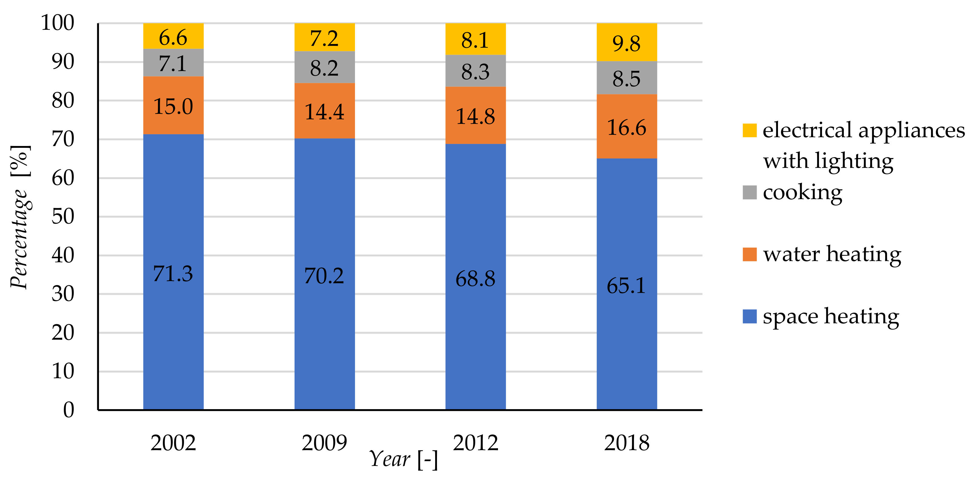
1. Introduction
- geometrical parameters (including the shape factor or the ratio of the window area to the wall area),
- urban conditions (determining the orientation towards cardinal directions and shadows from surrounding buildings, elements of small architecture and greenery),
- material and technical solutions (thermal–physical properties of building materials, accumulation capacities and variable solar energy transmission parameters of transparent partitions),
- installation solutions (type of ventilation, heating, and hot water preparation system as well as the possibility of their regulation and intelligent energy and building management) and internal equipment.
2. Materials and Methods
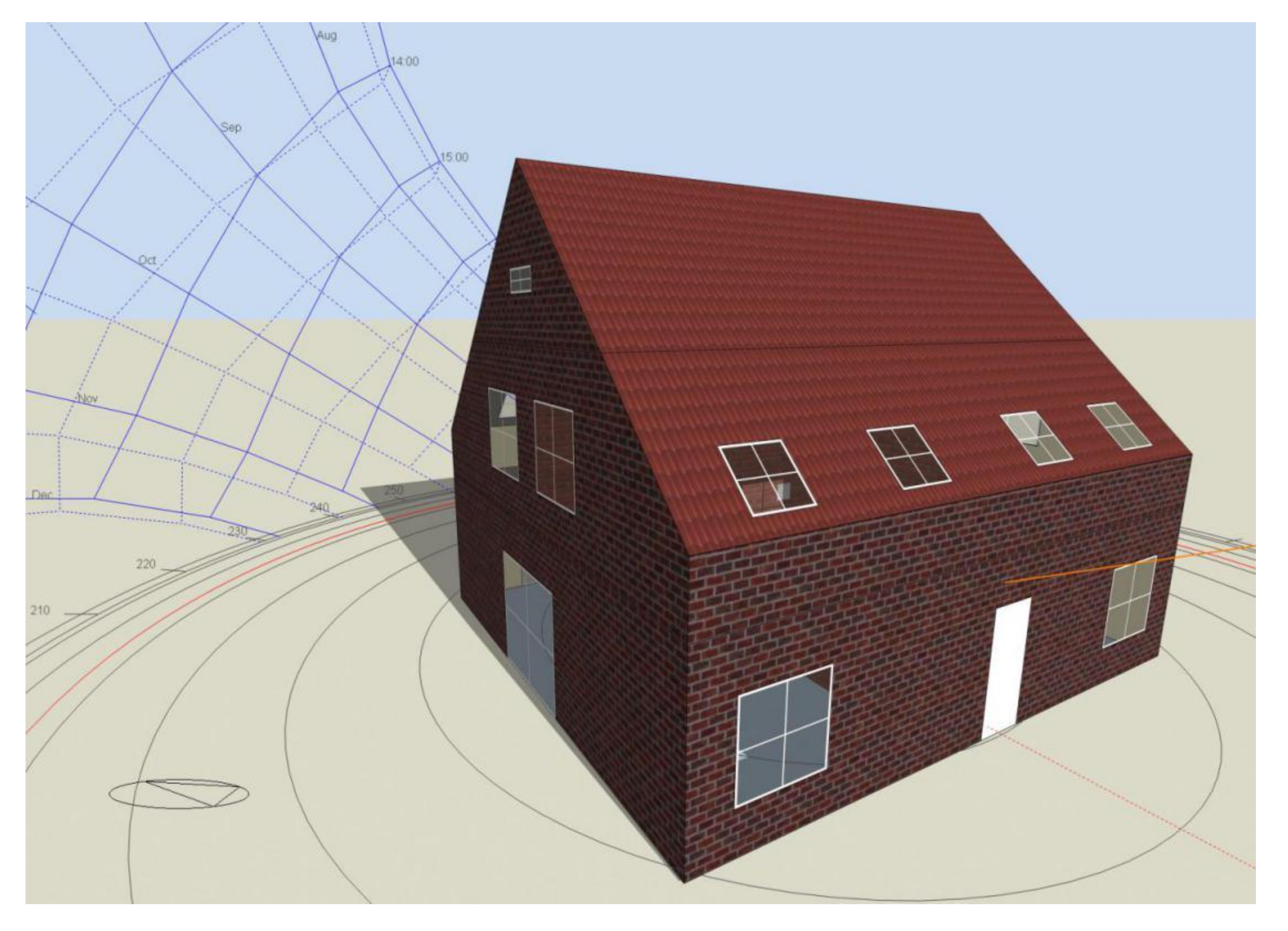
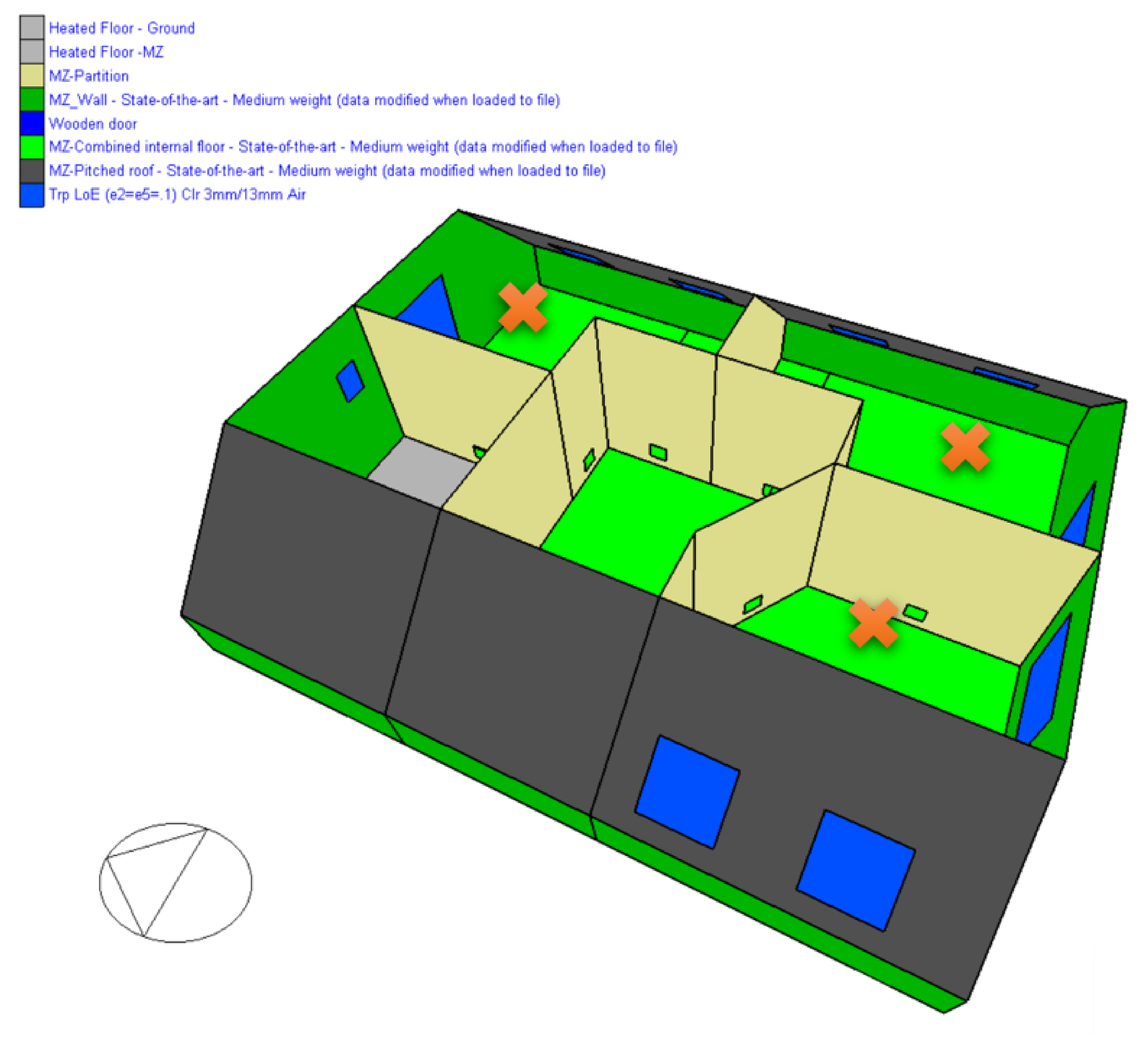
2.1. Description of the Single-Family House and the Assumptions Used in the Calculations
- Latitude: 53.1°; Longitude: 23.17°; elevation above sea level—151 m.
- Annual average outdoor air temperature: 6.92 °C, maximal difference monthly average outdoor temperature: 22.17 °C,
- One person consumes 50 L of domestic hot water daily, which gives 72.99 m3 annual consumption for 4 people; peak flow rate—0.00000216 m3/s.
- In order to assess thermal comfort in rooms and heat gains from people, the insulation of residents’ clothing was assumed to be 1clo during the winter and 0.5 during the summer; activity—manual work; CO2 generation rate—0.0000000382 (m3/s−W).
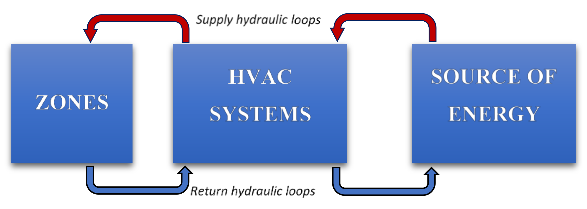
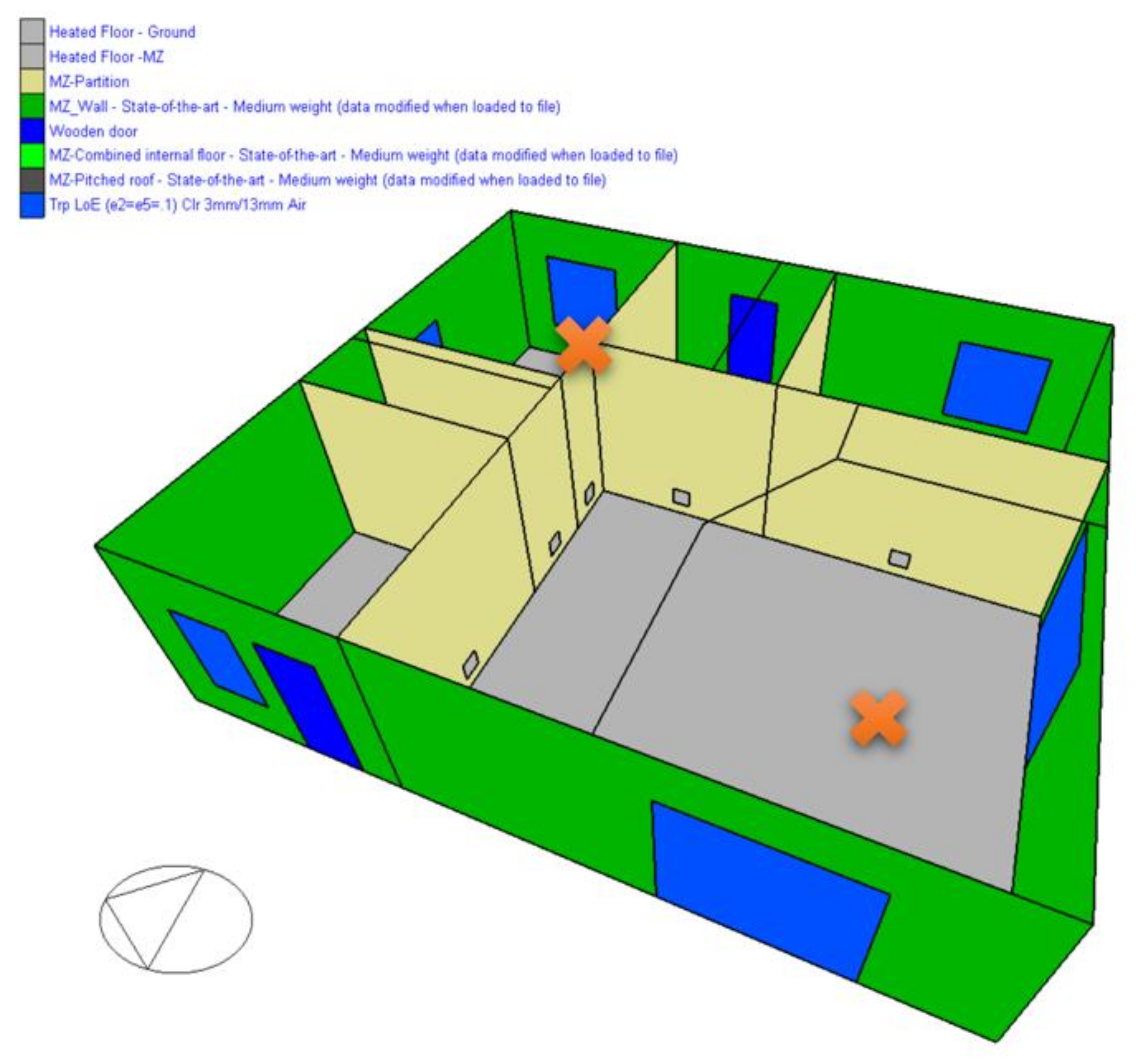
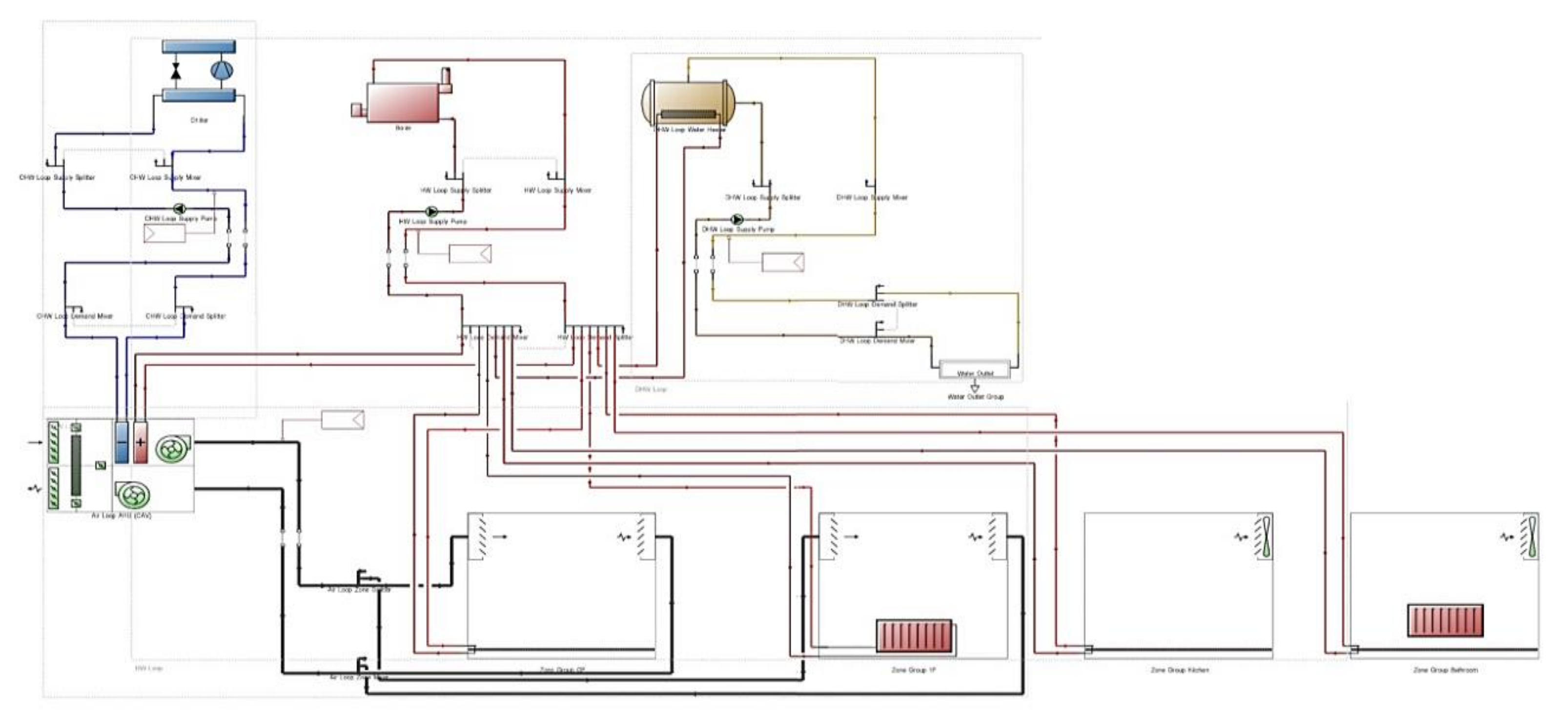
2.2. Description of the Software Used for Energy Simulations and Single-Family House Computational Model
2.3. Mathematical Model of the Final Energy Demand for a Selected Residential Building
2.4. List of Parameters for Assessing the Indoor Air Qualit and Scenarios under Test
- Carbon dioxide concentration,
- Indoor air humidity,
- Predicted mean vote (PMV)—index from the static model of thermal comfort, which was developed by Fanger [33],
- Operative temperature TO, defined according to Equation (8):where TMR—mean radiant temperature, TA—air temperature and v—air velocity.
3. Results and Discussion
3.1. Analysis of the Examined Relationship Based on the Mathematical Model
3.2. Example Application of the Developed Mathematical Model
X3 = [2 × 5 − (7 + 1)]/(7 − 1) = 0.3333; X4a = [2 × 1 − (3 + 1)]/(3 − 1) = −1;
X4b = [2 × 2 − (3 + 1)]/(3 − 1) = 0.
- With coal boiler:Ya = 1315.97− 889.82·0 + 41.42·0.6167 + 300.53·0.3333 − 159.95·(−1) + 28.24·0·0.6167 − 99.02·0·0.3333 + 85.79·0·(−1) + 19.27·0.6167·0.3333 − 5.21·0.6167·(−1) − 33.24·0.3333·(−1) − 2.41·02 − 38.73·0.33332 + 228.07·(−1)2 = 1843.65 kWh/month;
- With a gas boiler:Yb = 1315.97 − 889.82·0 + 41.42·0.6167 + 300.53·0.3333 − 159.95·0 + 28.24·0·0.6167 − 99.02·0·0.3333 + 85.79·0·0 + 19.27·0.6167·0.3333 − 5.21·0.6167·0 − 33.24·0.3333·0 − 2.41·02 − 38.73·0.33332 + 228.07·02 = 1441.34 kWh/month.
3.3. Analysis of Indoor Air Quality and Thermal Comfort
4. Conclusions
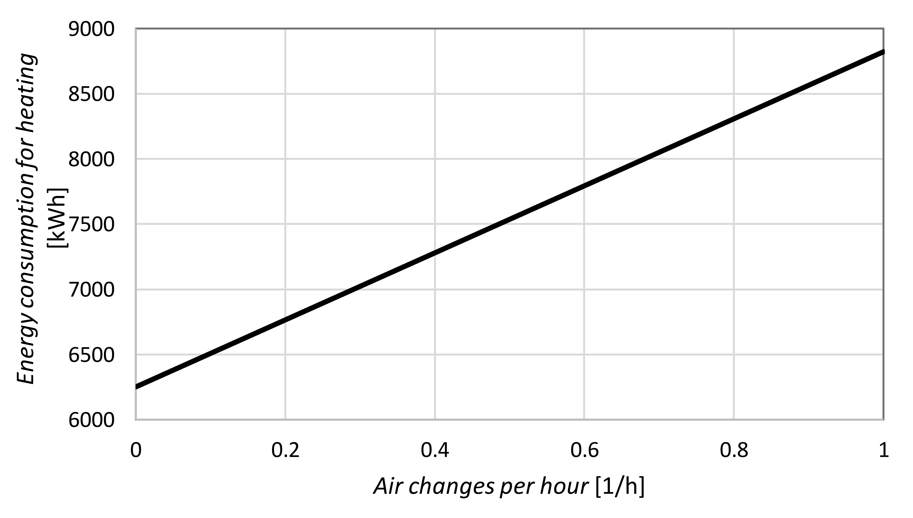
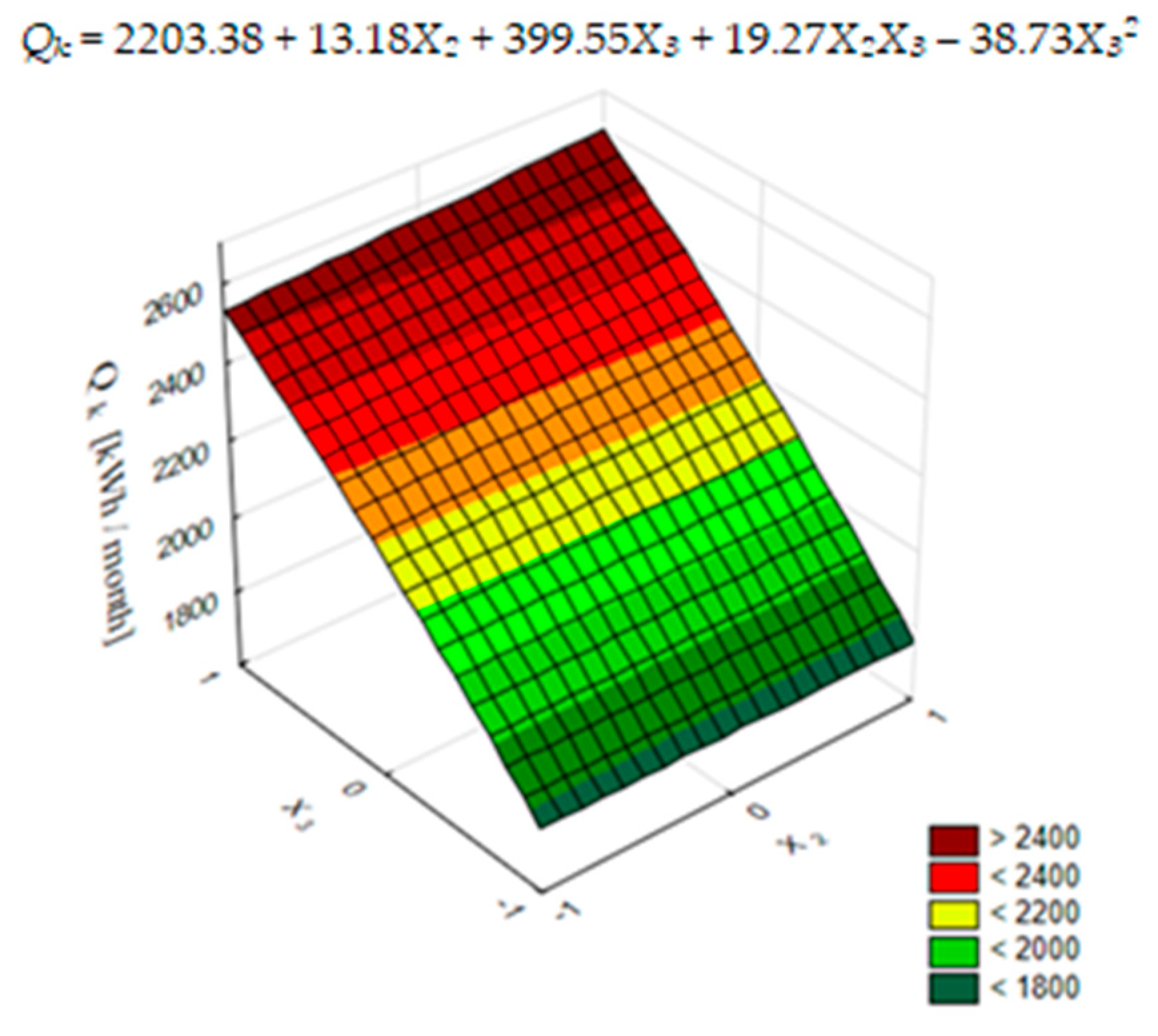
- It was found that preventive self-isolation of residents noticeably increases final energy demand for space heating and heating domestic hot water in inhabited buildings. When changing the length of the self-isolation period of four residents in the selected building from 0 to 31 days, there is a linear increase of Qk by about 6.5%. On the other hand, when the number of inhabitants in this building changes from one to four people, Qk increases by 34.7%, while with four to seven people, Qk increases by 26.9%. On the basis of the developed model (4), it is possible to determine the monthly demand for final energy of a single-family residential building with a form and climatic conditions similar to the analyzed ones.
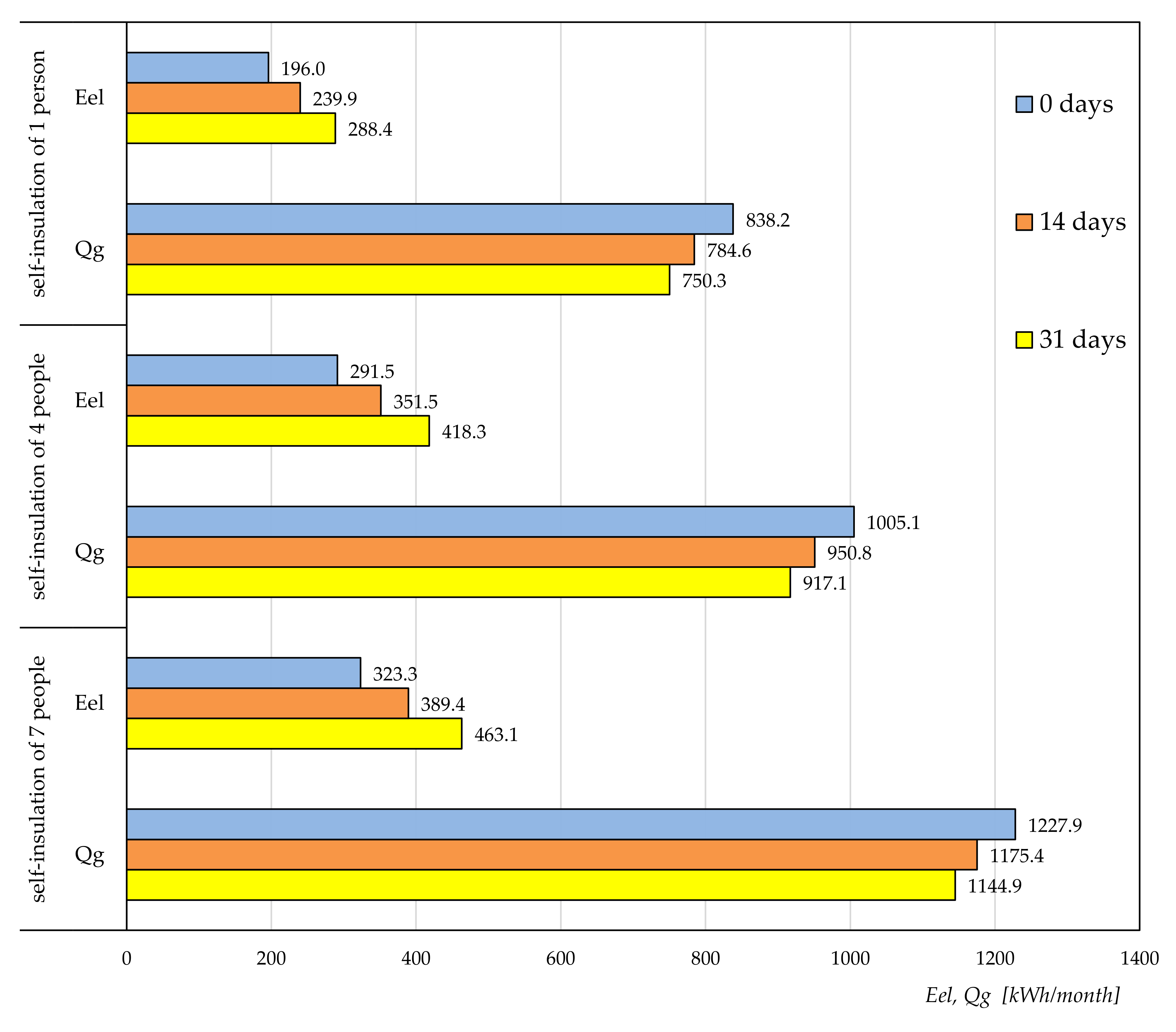
- It can also be said that during periods of residents’ self-isolation, there are changes in the structure of building energy demand. With the increase in the length of the self-isolation period from 0 to 31 days, the demand for electricity for the operation of various types of electrical equipment Eel increases by about 40–42%, while the demand for energy contained in the fuel burned Qg decreases by about 7–10% for each number of residents remaining in self-isolation.
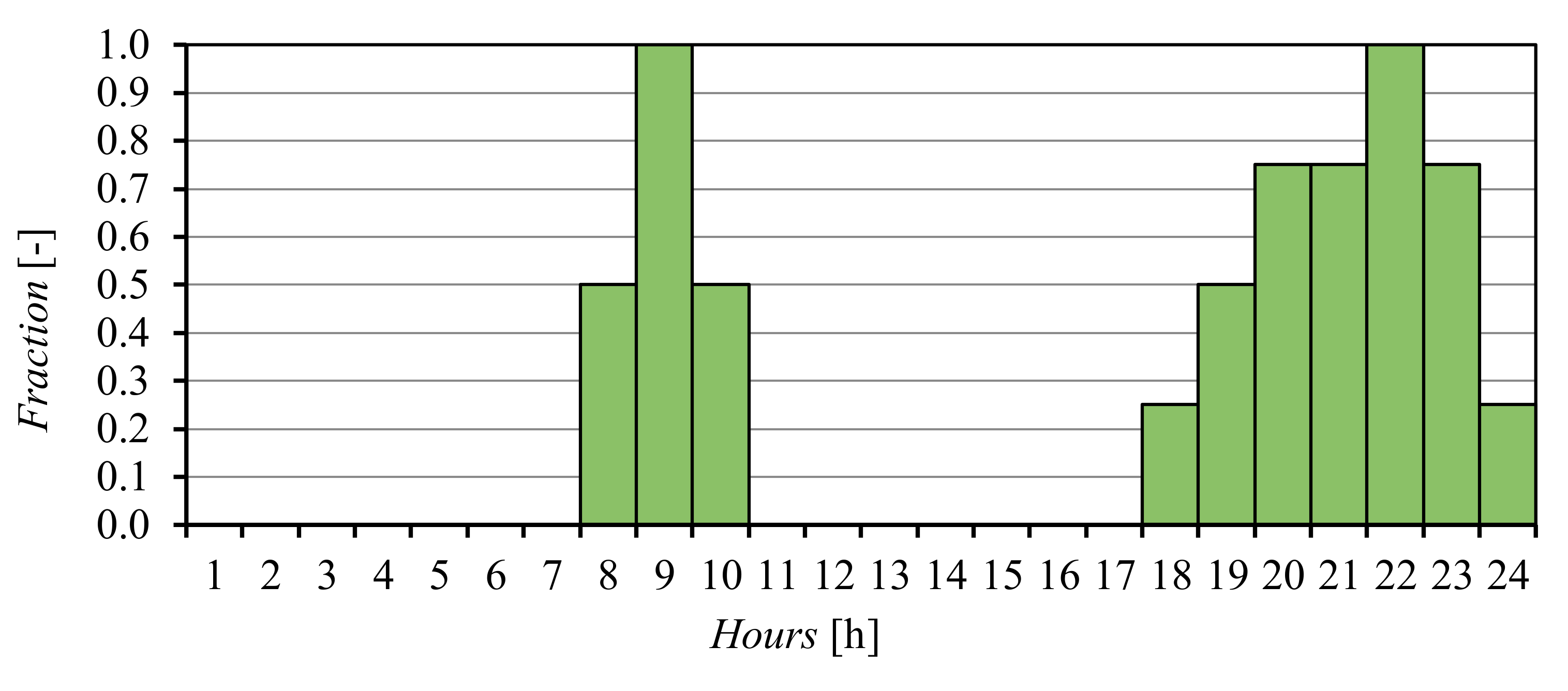
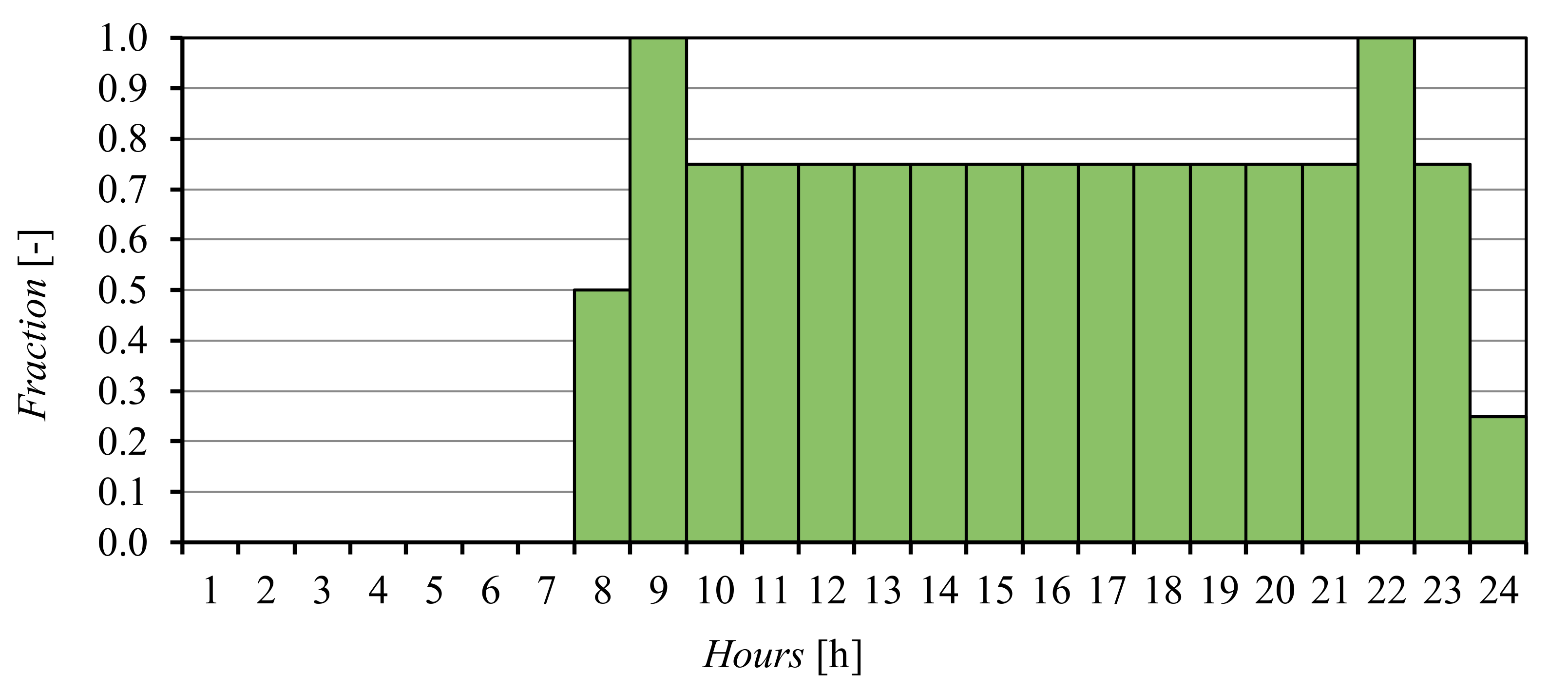
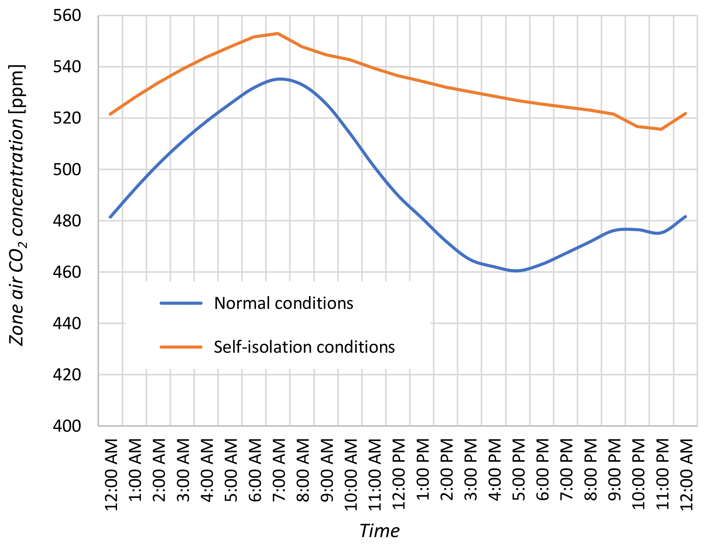
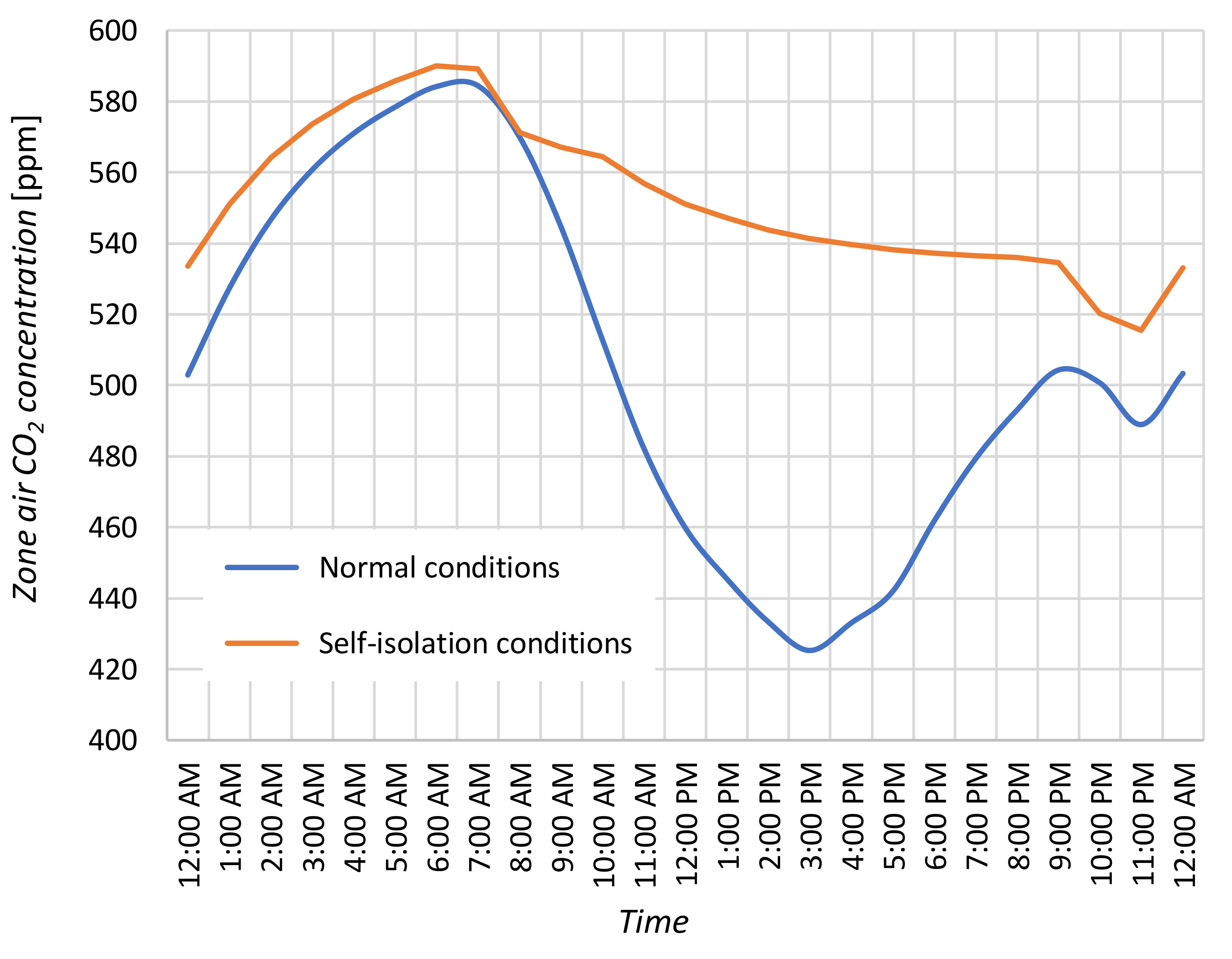
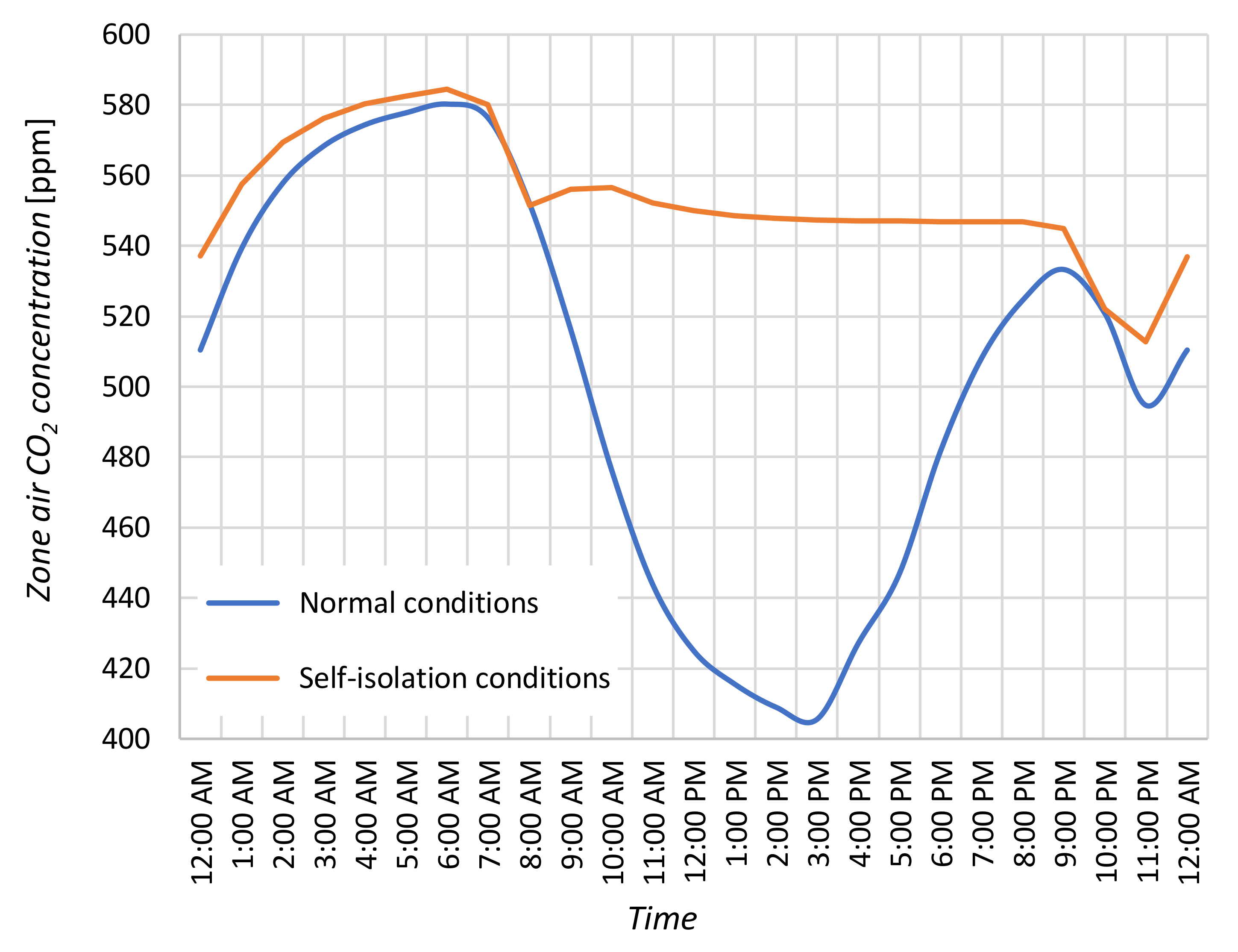
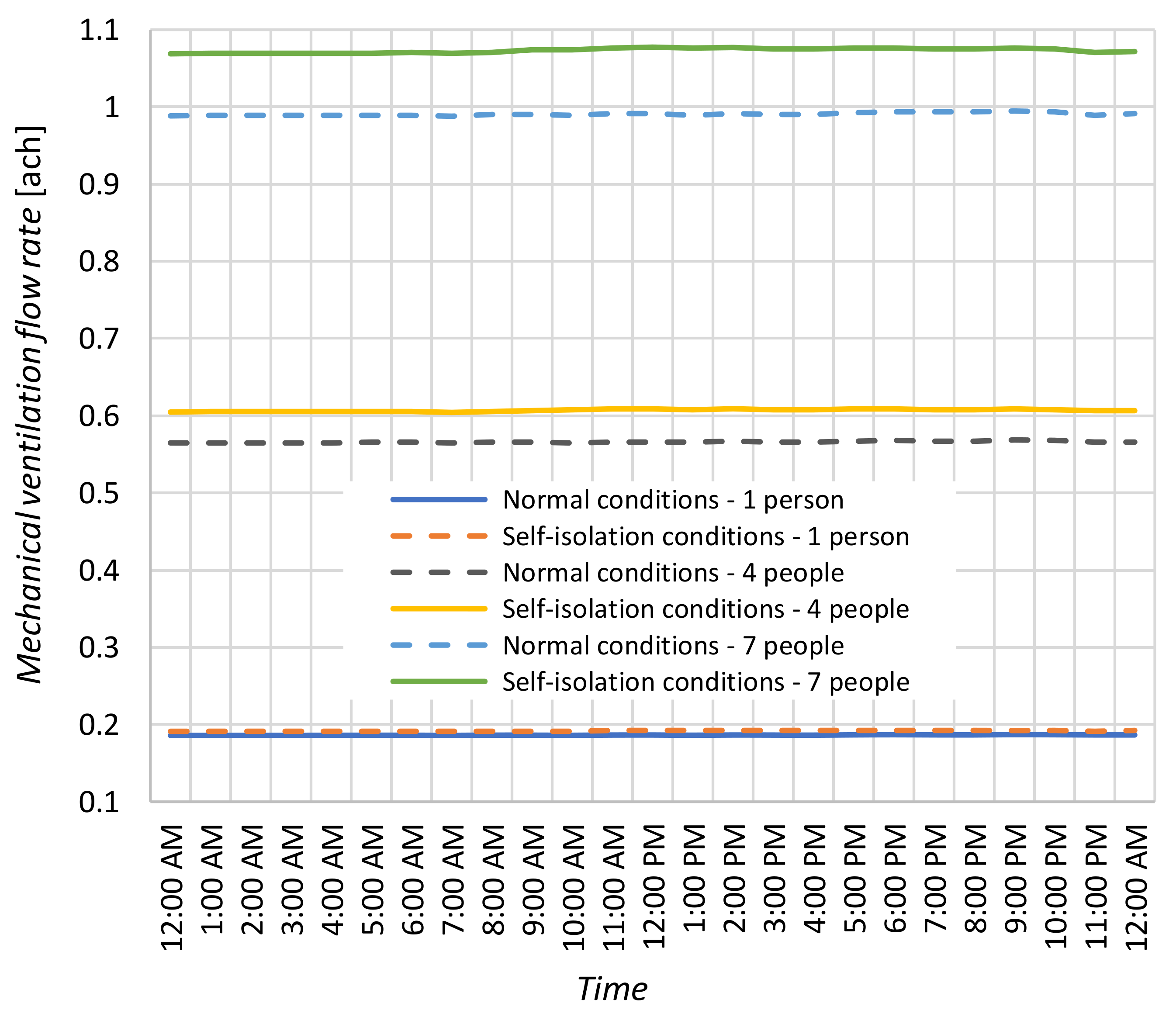
- The article also analyses whether the self-isolation of residents can affect the quality of indoor air. As shown by the simulation results, the IAQ remained at a similar level, within the recommended range. It was the result of using mechanical ventilation and changing the air flow rate VV as a function of the number of inhabitants and the schedule of their stay at home. The increase in the number of inhabitants from one to four and to seven required a triple and fivefold increase in the value of VV, respectively. The only negative consequence of the operation of ventilation system was too low moisture content in the indoor air.
Author Contributions
Funding
Conflicts of Interest
Abbreviations
| heat capacity of the zone | |
| zone air temperature | |
| t | time |
| Nl | number of internal loads |
| internal load | |
| Ns | number of zone surfaces |
| hi | convective heat transfer coefficient |
| Ai | area of zone surface |
| Tsi | temperature of zone surface |
| inter-zone mass flow rate | |
| cp | air specific heat |
| Tsi | temperature of zone surface |
| Nz | number of adjacent zones |
| Tzi | temperature of adjacent zone |
| infiltration mass flow rate | |
| Tamb | ambient air temperature |
| HVAC system mass flow rate | |
| Ts | supply air temperature |
References
- Global Energy Statistical Yearbook—2019 Edition—Enerdata. Available online: https://yearbook.enerdata.net/total-energy/world-consumption-statistics.html (accessed on 20 May 2020).
- Global Energy Review 2020—Analysis IEA. Available online: https://www.iea.org/reports/global-energy-review-2020 (accessed on 20 May 2020).
- Global Energy Review 2020—The impacts of the COVID-19 Crisis on Global Energy Demand and CO2 Emissions; IEA’s Flagship Report—April 2020. Available online: https://www.iea.org/reports/global-energy-review-2020/electricity (accessed on 20 May 2020).
- Economidou, M.; Todeschi, V.; Bertoldi, P.; D’Agostino, D.; Zangheri, P.; Castellazzi, L. Review of 50 years of EU energy efficiency policies for buildings. Energy Build. 2020, 225. [Google Scholar] [CrossRef]
- Bouzarovski, S.; Herrero, S.T.; Petrova, S.; ÜrgeVorsatz, D. Unpacking the spaces and politics of energy poverty: Path-dependencies, deprivation and fuel switching in post-communist Hungary. Local Environ. 2016, 21, 1151–1170. [Google Scholar] [CrossRef]
- Tsemekidi-Tzeiranaki, S.; Bertoldi, P.; Labanca, N.; Castellezzi, L.; Serrenho, T.; Economidou, M.; Zangheri, P. Energy Consumption and Energy Efficiency Trends in the EU-28 for the Period. 2000–2016 EUR 29473 EN; Publications Office of the European Union: Luxembourg, 2018. [Google Scholar]
- Reuter, M.; Patel, M.K.; Eichhammer, W. Applying ex post index decomposition analysis to final energy consumption for evaluating European energy efficiency policies and targets. Energy Effic. 2019, 12, 1329–1357. [Google Scholar] [CrossRef]
- Tsemekidi-Tzeiranaki, S.; Bertoldi, P.; Diluiso, F.; Castellezzi, L.; Economidou, M.; Labanca, N.; Serrenho, T.; Zangher, P. Analysis of the EU residential energy consumption: Trends and determinant. Energies 2019, 12, 1065. [Google Scholar] [CrossRef]
- Statistics Poland Household Energy Consumption in 2018. Available online: https://stat.gov.pl/obszary-tematyczne/srodowisko-energia/energia/zuzycie-energii-w-gospodarstwach-domowych-w-2018-roku,2,4.html (accessed on 20 May 2020).
- National Plan for Increasing the Number of Nearly Zero-Energy Buildings as Required by Directive 2010/31/EU on the Energy Performance of Buildings (EPBD Recast)—Poland. 2015. Available online: https://eli.gov.pl/api/acts/MP/2015/614/text/I/M20150614.pdf (accessed on 25 May 2020).
- BPIE; Staniaszek, D.; Firląg, S.Z. Financing Building Energy Performance Improvement in Poland. Status Report. 2016. Available online: http://bpie.eu/publication/financing-building-energy-performance-improvement-in-poland-status-report/ (accessed on 20 May 2020).
- Grudzińska, M.; Ostańska, A.; Życzyńska, A. Low Energy and Passive Buildings; Medium Group: Warsaw, Poland, 2017. [Google Scholar]
- Chen, S.; Zhang, G.; Xia, X.; Setunge, S.; Shi, L. A review of internal and external influencing factors on energy efficiency design of buildings. Energy Build. 2020, 216, 109944. [Google Scholar] [CrossRef]
- Pacheco, R.; Ordonez, J.; Martinez, G. Energy efficient design of building: A review. Ren. Sustain. Energy Rev. 2012, 16, 3559–3573. [Google Scholar] [CrossRef]
- Goia, F. Search for the optimal window-to-wall ratio in office buildings in different European climates and the implications on total energy saving potential. Sol. Energy 2016, 132, 467–492. [Google Scholar] [CrossRef]
- Obrecht, T.; Vesn, M.P.; Leskovar, Ž. Influence of the orientation on the optimal glazing size for passive houses in different European climates (for non-cardinal directions). Sol. Energy 2019, 189, 15–25. [Google Scholar] [CrossRef]
- Brom, P.; Hansen, A.R.; Gram-Hanssen, K.; Meijer, A.; Visscher, H. Variances in residential heating consumption – Importance of building characteristics and occupants analysed by movers and stayers. Appl. Energy 2019, 250, 713–728. [Google Scholar] [CrossRef]
- Santin, O.G. Behavioural patterns and user profiles related to energy consumption for heating. Energy Build. 2011, 43, 2662–2672. [Google Scholar] [CrossRef]
- Nguyen, T.A.; Aiello, M. Energy intelligent buildings based on user activity: A survey. Energy Build. 2016, 56, 244–257. [Google Scholar] [CrossRef]
- Main Office of Building Control. Construction market in Poland in 2018. 2018. Available online: https://www.gunb.gov.pl/aktualnosc/ruch-budowlany-w-2018-r (accessed on 28 April 2020).
- Statistics Poland. Statistical Analyses. Construction Result in 2019; Statistical Office in Lublin: Warsaw, Poland, 2020; pp. 33–34. [Google Scholar]
- Report on the Construction of Houses in Poland in 2018; Oferteo.pl Service Report. Available online: https://www.nieruchomosci.egospodarka.pl/154042,Budowa-domow-w-Polsce-2018,1,80,1.html (accessed on 26 October 2020).
- EnergyPlus™ Version 9.3.0 Documentation. Engineering Reference; U.S. Department of Energy: Washington, DC, USA, 27 March 2020. Available online: https://www.google.com/url?sa=t&rct=j&q=&esrc=s&source=web&cd=&ved=2ahUKEwi_5aqBpbftAhUllosKHQCPDR0QFjAAegQIBRAC&url=https%3A%2F%2Fenergyplus.net%2Fsites%2Fall%2Fmodules%2Fcustom%2Fnrel_custom%2Fpdfs%2Fpdfs_v9.3.0%2FEngineeringReference.pdf&usg=AOvVaw1drV7NwKPCki4unAIb0UZ6 (accessed on 5 December 2020).
- Groth, C.C.; Lokmanhekim, M.S.A. New technique for the calculation of shadow shapes and areas by digital computer. In Proceedings of the Second Hawaii International Conference on System Sciences, Honolulu, HI, USA, 22–24 January 1969. [Google Scholar]
- Walton, G.N. The Thermal Analysis Research Program. Reference Manual Program. (TARP); National Bureau of Standards (now National Institute of Standards and Technology): Washington, DC, USA, 1983. [Google Scholar]
- Hendron, R.; Anderson, R.; Christensen, C.; Eastment, M.; Reeves, P. Development of an Energy Savings Benchmark for All Residential End-Uses. In Proceedings of the Development of an Energy Savings Benchmark for All Residential End-Uses SimBuild, Boulder, CO, USA, 4–6 August 2004. [Google Scholar]
- Burch, J.; Christensen, C. Towards development of an algorithm for mains water temperature. In Proceedings of the ASES Annual Conference, Cleveland, OH, USA, 10–12 October 2007. [Google Scholar]
- EnergyPlus—Weather Data by Location. 2020. Available online: https://energyplus.net/weather (accessed on 10 May 2020).
- Gutenbaum, J. Modelowanie Matematyczne Systemów; EXIT: Warszawa, Poland, 2003. (In Polish) [Google Scholar]
- Korzyński, M. Metodyka Eksperymentu. Planowanie, Realizacja i Statystyczne Opracowanie Wyników Eksperymentów Technologicznych; WNT: Warszawa, Poland, 2006. (In Polish) [Google Scholar]
- Durakovic, B. Design of experiments application, concepts, examples: State of the art. Per. Eng. Nat. Sci. 2017, 5, 421–439. [Google Scholar] [CrossRef]
- Hartmann, K.; Lezki, E.; Schär, W. Statistische Versuchsplanung und–Auswertung in der Stoffwirtschaft; VEB: Leipzig, Germany, 1977. (In German) [Google Scholar]
- Fanger, P.O. Thermal comfort. In Analysis and Applications in Environmental Engineering; Danish Technical Press: Copenhagen, Denmark, 1970. [Google Scholar]
- Boerstra, A. New health & comfort promoting CEN standard. REHVA J. 2019, 56, 8. Available online: https://www.rehva.eu/rehva-journal/chapter/new-health-comfort-promoting-cen-standard (accessed on 7 November 2020).


| Area (m2) | Conditioned (Y/N) | Volume (m3) | Gross Wall Area (m2) | Window Glass Area (m2) | |
|---|---|---|---|---|---|
| Groundfloor | |||||
| Toilet | 5.25 | No | 15.75 | 4.50 | 0.17 |
| Room | 15.75 | Yes | 47.25 | 24 | 4.03 |
| Saloon | 45.00 | Yes | 135.0 | 40.5 | 9.80 |
| Kitchen | 15.75 | Yes | 47.25 | 24 | 2.02 |
| First Floor | |||||
| Corridor | 20.55 | No | 55.65 | 3.00 | 0.00 |
| Bedroom1 | 23.38 | Yes | 59.13 | 17.75 | 3.71 |
| Bedroom3 | 20.32 | Yes | 51.98 | 16.75 | 3.71 |
| Bedroom2 | 23.8 | Yes | 60.4 | 17.9 | 3.71 |
| Bathroom | 16.45 | Yes | 42.35 | 15.6 | 0.17 |
| Attic | |||||
| Attic | 60.5 | No | 83.19 | 15.12 | 0.55 |
| Conditioned Total | 160.45 | 443.35 | 156.5 | 27.14 | |
| Unconditioned Total | 86.3 | 154.59 | 22.62 | 0.72 | |
| Total | 246.75 | 597.94 | 179.12 | 27.86 | |
| Parameter | Unit | Total | North | East | South | West |
|---|---|---|---|---|---|---|
| Gross Wall Area | m2 | 179.12 | 50.06 | 35.00 | 60.56 | 33.50 |
| Window Opening Area | m2 | 25.26 | 5.36 | 4.50 | 10.14 | 5.26 |
| Gross Window-Wall Ratio | % | 14.10 | 10.70 | 12.86 | 16.74 | 15.71 |
| No | m | τ | N | r | Qk (Yi) |
|---|---|---|---|---|---|
| X1 | X2 | X3 | X4 | kWh/month | |
| 1 | 1 −1 | 0 −1 | 1 −1 | 1 −1 | 2200.03 |
| 2 | 5 1 | 0 −1 | 1 −1 | 1 −1 | 388.29 |
| 3 | 1 −1 | 31 1 | 1 −1 | 1 −1 | 2207.07 |
| 4 | 5 1 | 31 1 | 1 −1 | 1 −1 | 492.77 |
| 5 | 1 −1 | 0 −1 | 7 1 | 1 −1 | 3065.53 |
| 6 | 5 1 | 0 −1 | 7 1 | 1 −1 | 795.85 |
| 7 | 1 −1 | 31 1 | 7 1 | 1 −1 | 3128.65 |
| 8 | 5 1 | 31 1 | 7 1 | 1 −1 | 1016.17 |
| 9 | 1 −1 | 0 −1 | 1 −1 | 3 1 | 1793.92 |
| 10 | 5 1 | 0 −1 | 1 −1 | 3 1 | 304.04 |
| 11 | 1 −1 | 31 1 | 1 −1 | 3 1 | 1799.66 |
| 12 | 5 1 | 31 1 | 1 −1 | 3 1 | 385.86 |
| 13 | 1 −1 | 0 −1 | 7 1 | 3 1 | 2499.65 |
| 14 | 5 1 | 0 −1 | 7 1 | 3 1 | 623.18 |
| 15 | 1 −1 | 31 1 | 7 1 | 3 1 | 2551.12 |
| 16 | 5 1 | 31 1 | 7 1 | 3 1 | 795.70 |
| 17 | 1 −1 | 14 0 | 4 0 | 2 0 | 2100.02 |
| 18 | 5 1 | 14 0 | 4 0 | 2 0 | 527.10 |
| 19 | 3 0 | 0 −1 | 4 0 | 2 0 | 1296.52 |
| 20 | 3 0 | 31 1 | 4 0 | 2 0 | 1335.56 |
| 21 | 3 0 | 14 0 | 1 −1 | 2 0 | 1024.56 |
| 22 | 3 0 | 14 0 | 7 1 | 2 0 | 1529.92 |
| 23 | 3 0 | 14 0 | 4 0 | 1 −1 | 1712.97 |
| 24 | 3 0 | 14 0 | 4 0 | 3 1 | 1375.10 |
| Factor Level | m (X1) | τ* (X2) | N (X3) | r (X4) |
|---|---|---|---|---|
| bottom (−1) | 1 | 0 | 1 | 1 |
| middle (0) | 3 | 15 | 4 | 2 |
| upper (+1) | 5 | 30 | 7 | 3 |
| range of factor change ΔXi | 2 | 15 | 3 | 1 |
| Analysed Factors | Values of Factors | The Scenarios under Test | ||||||||
|---|---|---|---|---|---|---|---|---|---|---|
| Energy Demand | Air Quality and Thermal Comfort | |||||||||
| Qk | Graph of the Dependence of Qk on τ and N | Eel, Qg | Example Application of the Developed Model | Relative Humidity | CO2 Concentration | PMV | Operative Temperature | Mechanical Ventilation | ||
| kWh/month | % | ppm | − | °C | ach | |||||
| the period (month) of the active pandemic phase m | January | + | + | − | − | − | − | − | − | − |
| March | + | − | + | + | + | + | + | + | + | |
| May | + | − | − | − | − | − | − | − | − | |
| the length of the self-isolation period of residents τ | 0 days | + | + | + | τ = 24 | + | + | + | + | + |
| 15 days | + | + | + | + | + | + | + | + | ||
| 30 days | + | + | + | − | − | − | − | − | ||
| the number of residents in the house N | 1 | + | + | + | N = 5 | + | + | + | + | + |
| 4 | + | + | + | + | + | + | + | + | ||
| 7 | + | + | + | + | + | + | + | + | ||
| type of energy source in the building r | coal-fueled boiler | + | − | − | + | − | − | − | − | − |
| gas boiler | + | + | + | + | − | − | − | − | − | |
| electric heating | + | − | − | − | − | − | − | − | − | |
| Relative Humidity (%) | CO2 Concentration (ppm) | Fanger Model PMV (−) | Operative Temperature (°C) | Mechanical Ventilation (ach) | |
|---|---|---|---|---|---|
| Normal Conditions—1 Person | 20.2 | 492 | −1.15 | 21.0 | 0.186 |
| Self-Isolation Conditions—1 Person | 20.5 | 534 | −1.10 | 21.2 | 0.191 |
| Normal Conditions—4 People | 20.8 | 504 | −1.13 | 21.1 | 0.564 |
| Self-Isolation Conditions—4 People | 21.0 | 554 | −1.05 | 21.4 | 0.605 |
| Normal Conditions—7 People | 21.1 | 502 | −1.13 | 21.1 | 0.987 |
| Self-Isolation Conditions—7 People | 21.4 | 555 | −1.05 | 21.4 | 1.069 |
Publisher’s Note: MDPI stays neutral with regard to jurisdictional claims in published maps and institutional affiliations. |
© 2020 by the authors. Licensee MDPI, Basel, Switzerland. This article is an open access article distributed under the terms and conditions of the Creative Commons Attribution (CC BY) license (http://creativecommons.org/licenses/by/4.0/).
Share and Cite
Jezierski, W.; Zukowski, M.; Sadowska, B. Analysis of the Impact of Self-Isolation of Residents during a Pandemic on Energy Demand and Indoor Air Quality in a Single-Family Building. Energies 2020, 13, 6470. https://doi.org/10.3390/en13236470
Jezierski W, Zukowski M, Sadowska B. Analysis of the Impact of Self-Isolation of Residents during a Pandemic on Energy Demand and Indoor Air Quality in a Single-Family Building. Energies. 2020; 13(23):6470. https://doi.org/10.3390/en13236470
Chicago/Turabian StyleJezierski, Walery, Mirosław Zukowski, and Beata Sadowska. 2020. "Analysis of the Impact of Self-Isolation of Residents during a Pandemic on Energy Demand and Indoor Air Quality in a Single-Family Building" Energies 13, no. 23: 6470. https://doi.org/10.3390/en13236470
APA StyleJezierski, W., Zukowski, M., & Sadowska, B. (2020). Analysis of the Impact of Self-Isolation of Residents during a Pandemic on Energy Demand and Indoor Air Quality in a Single-Family Building. Energies, 13(23), 6470. https://doi.org/10.3390/en13236470