Analytical Model for Predicting Productivity of Radial-Lateral Wells


Abstract
:1. Introduction
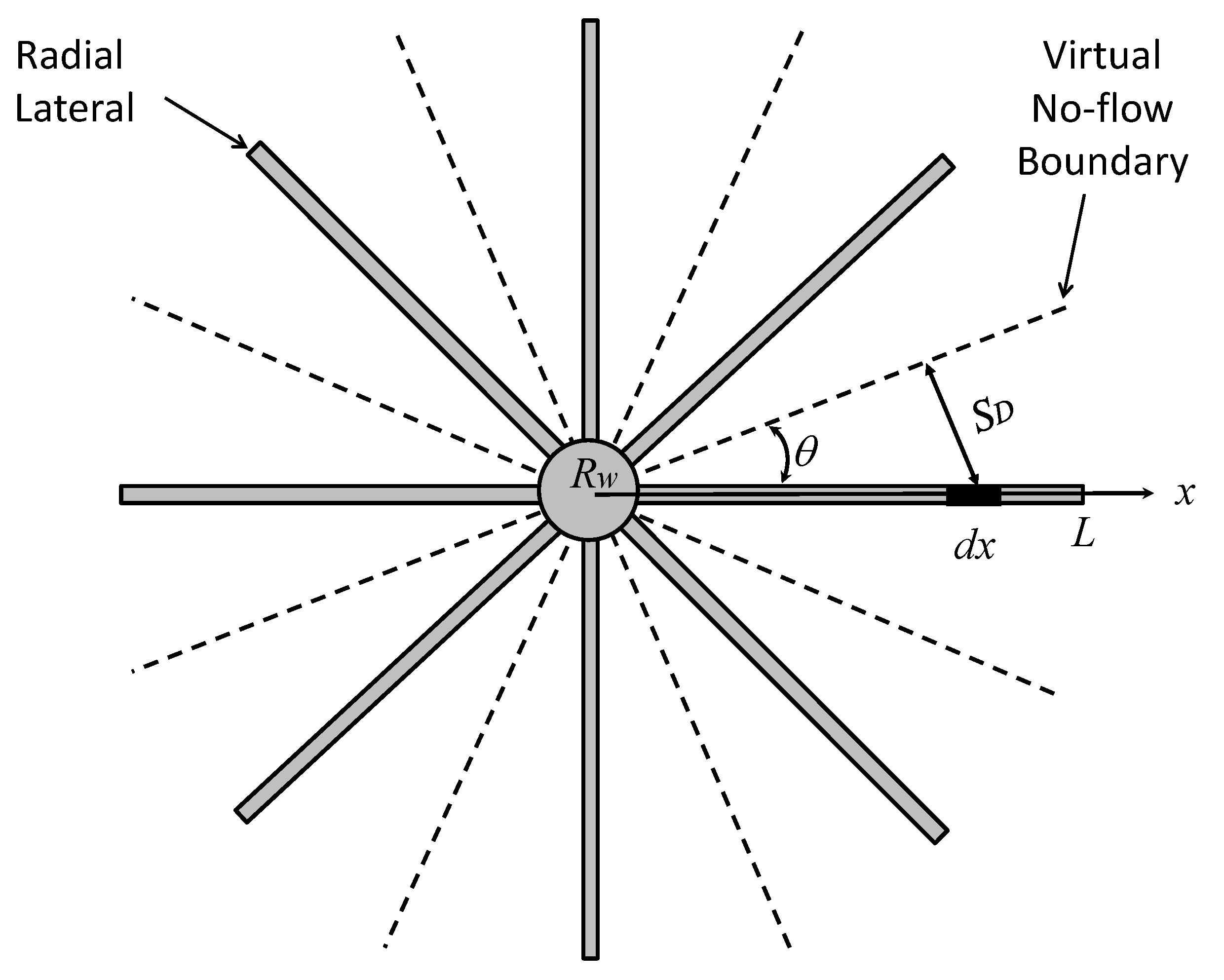
2. Mathematical Model
- Radial laterals are identical and distributed evenly in the drainage area.
- Pseudo-steady state flow conditions are reached within the lateral-reached drainage area.
- Single gas phase flow, and single oil phase flow, in dry gas reservoirs or in undersaturated oil reservoirs, respectively.
3. Model Validation
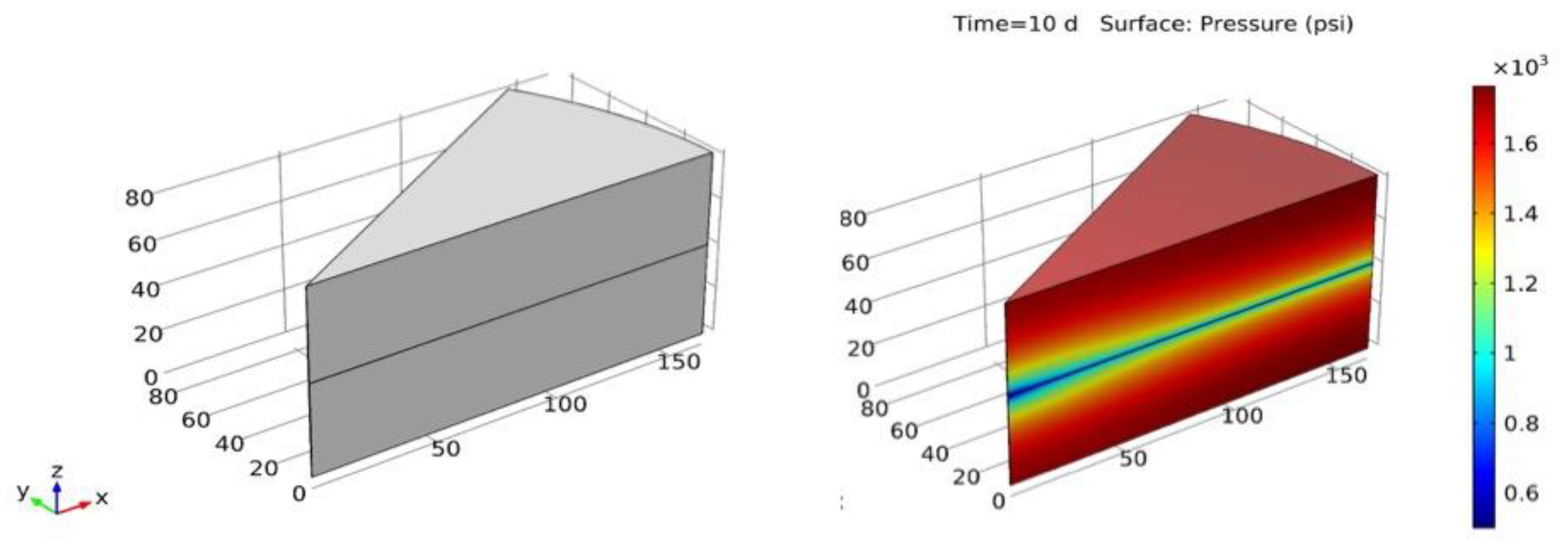
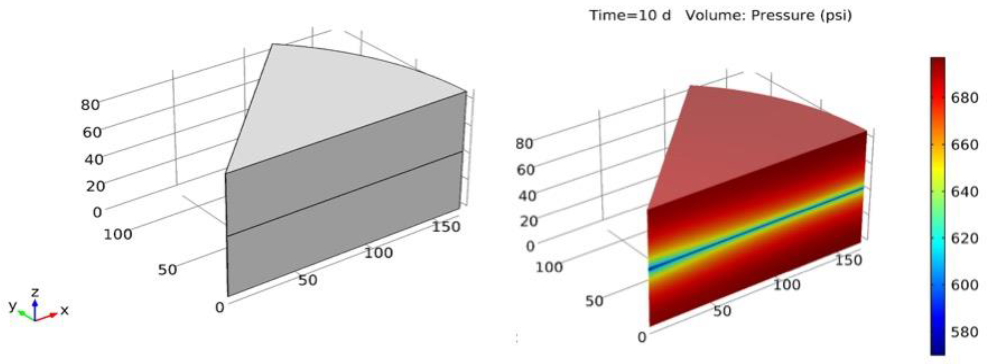
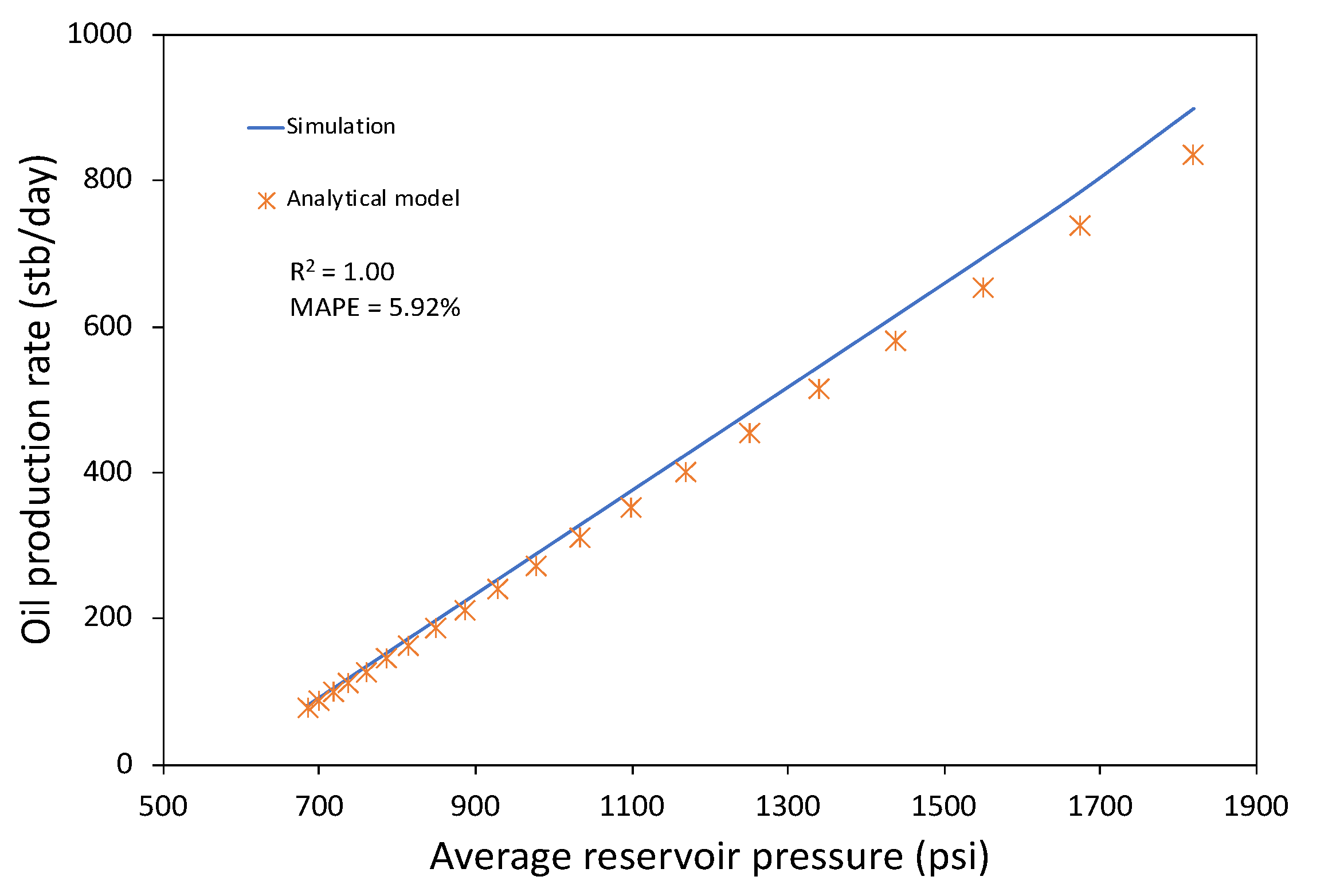
3.1. Numerical Simulation
3.2. Field Case Example
4. Parametric Analysis
5. Discussion
6. Conclusions
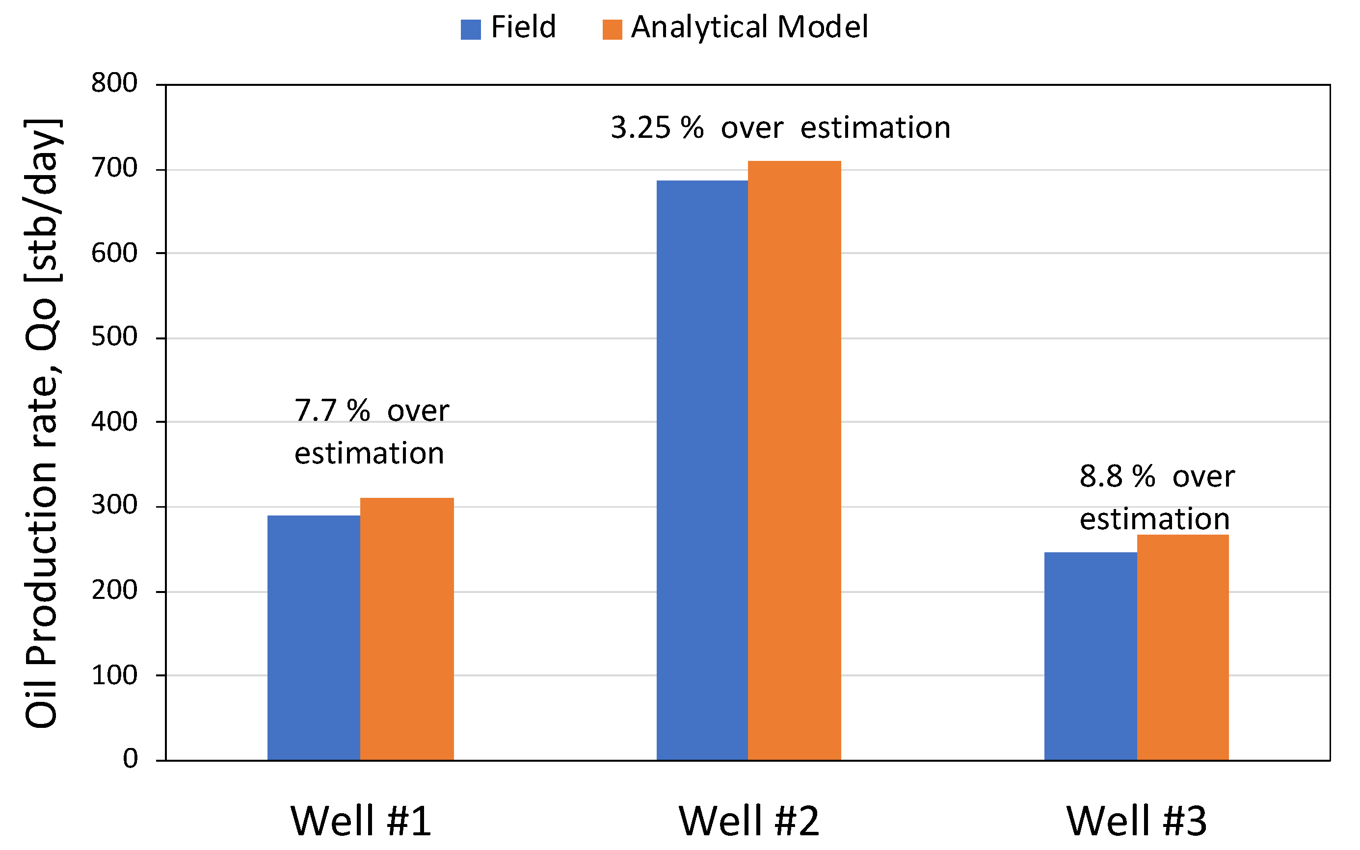
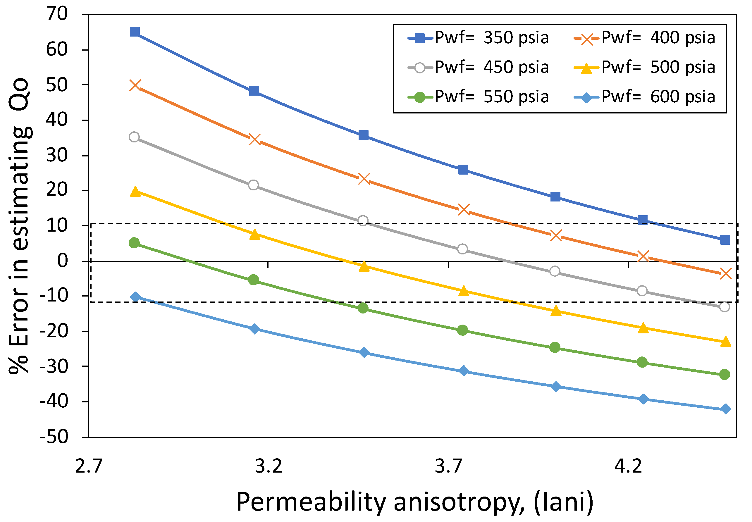
- The model overestimated the well production rate for wells 1, 2, and 3 by 7.7%, 3.25%, and 8.8%, respectively. The error is attributed to several sources, including (1) lack of data for well skin factor, (2) uncertainty of horizontal permeability (kH) in the well area, (3) uncertainty of permeability anisotropy (Iani), and (4) uncertainty in bottom hole pressure (pw).
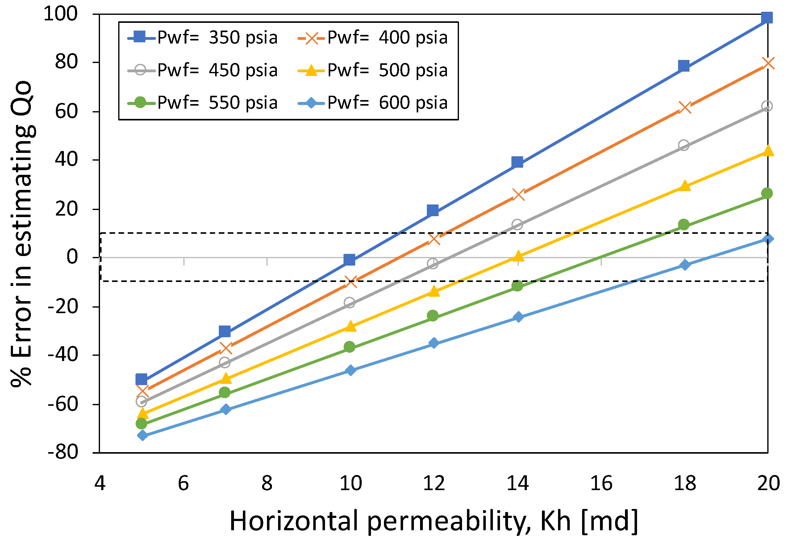
- Error analysis of uncertainties in kH, pw, and Iani showed that the model could predict productivity well with an acceptable error (10%) over practical ranges of these parameter values.
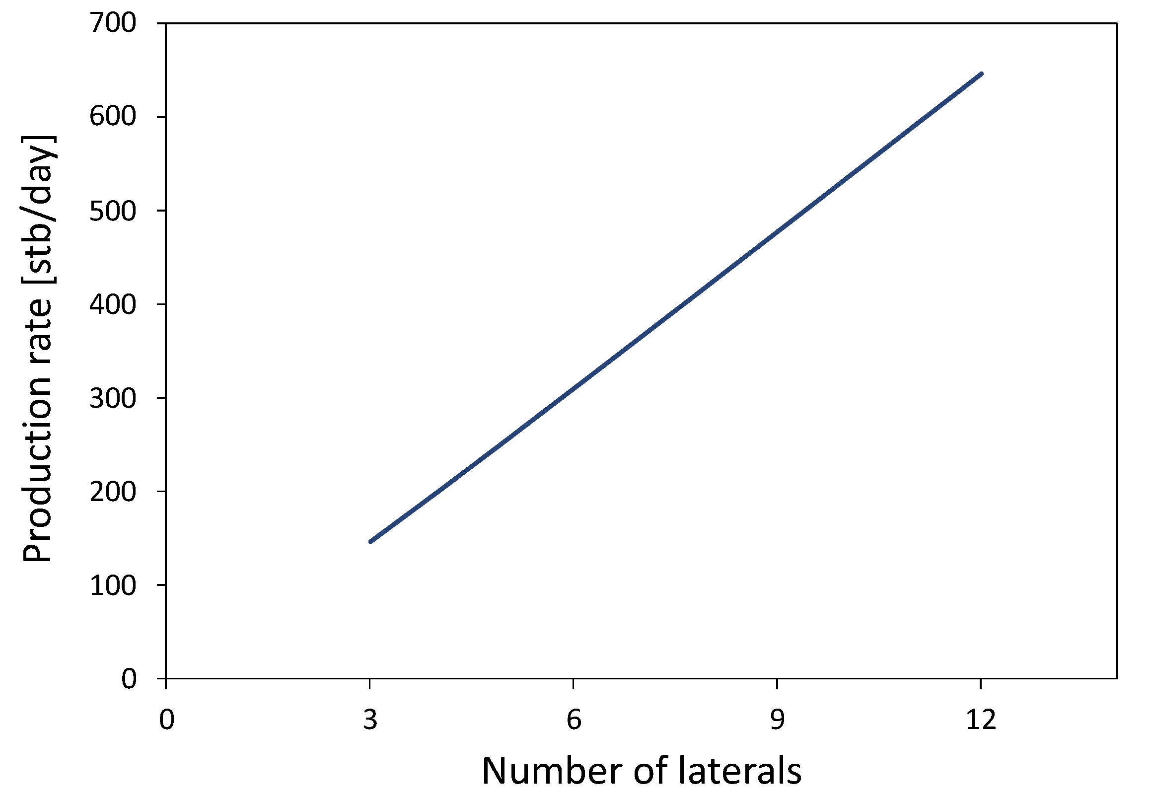
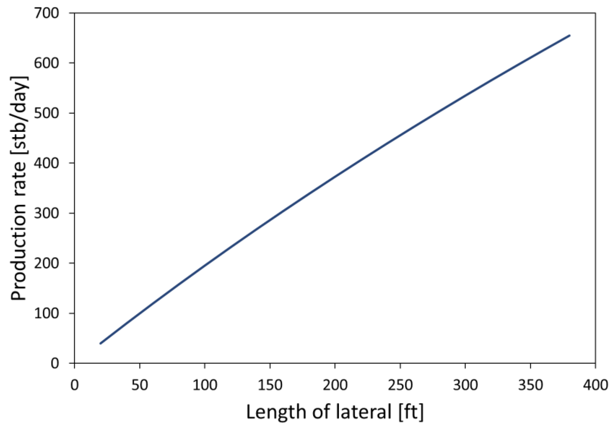
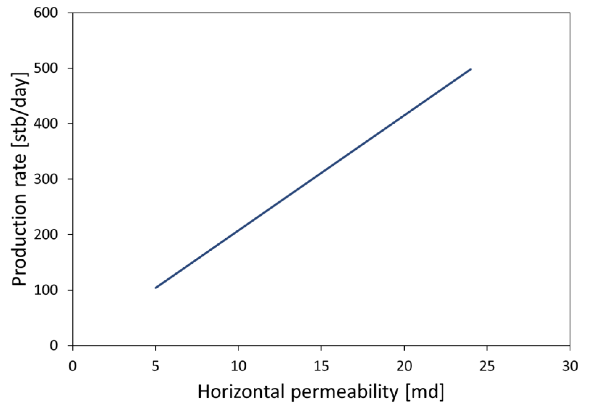
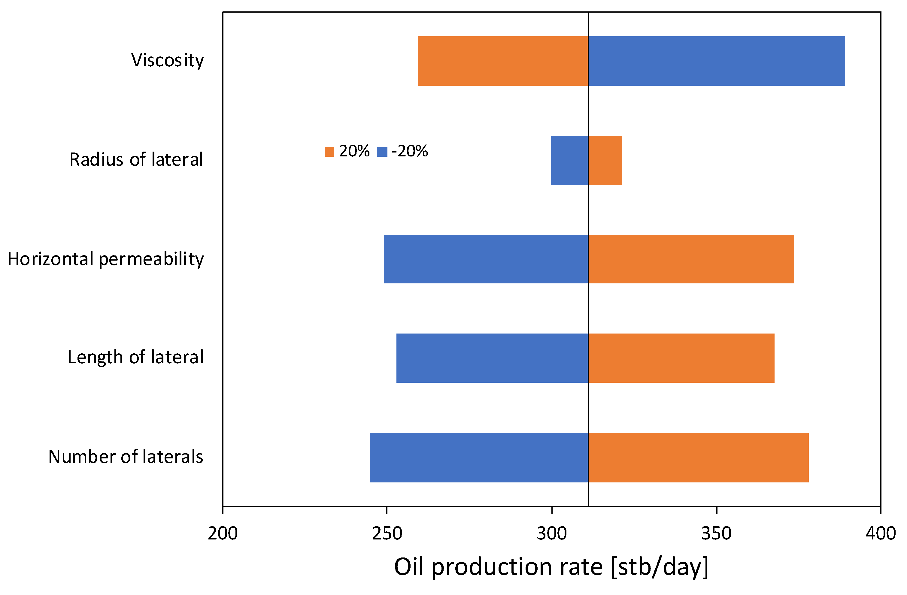
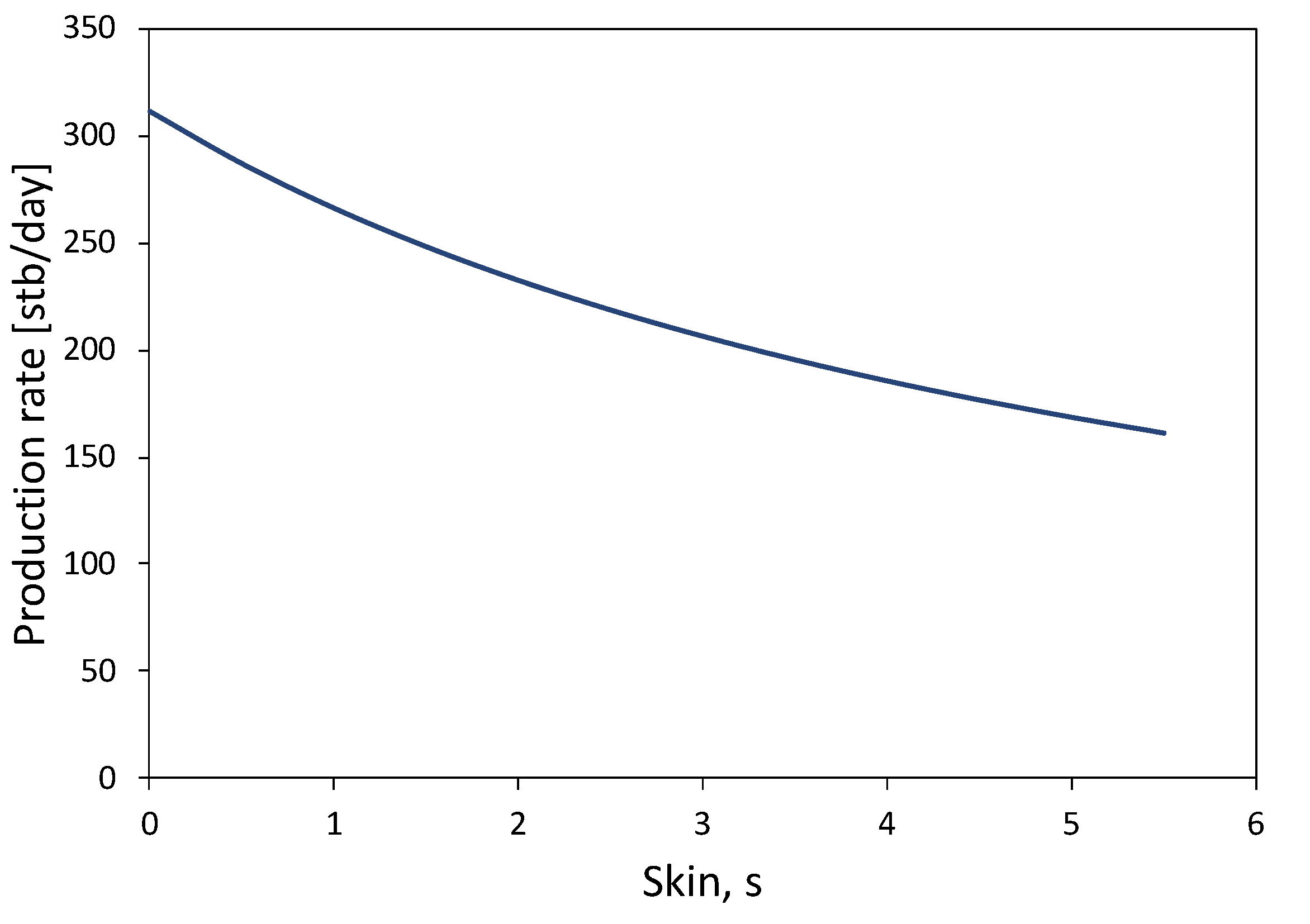
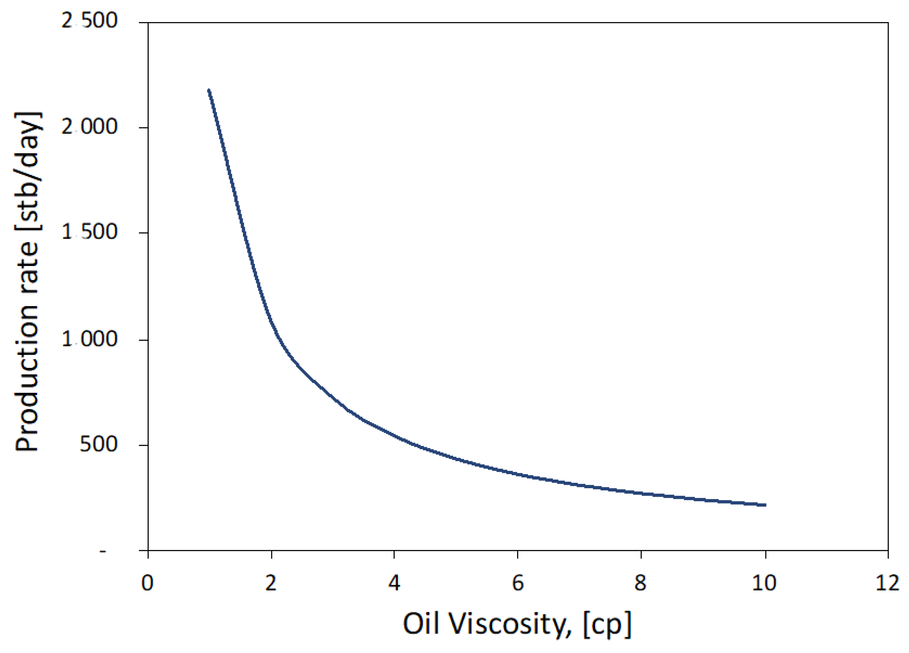
- Parameter sensitivity analyses showed that an increasing number of laterals, lateral length, and horizontal permeability would almost proportionally increase productivity. Well productivity is very sensitive to well skin factor and oil viscosity, but less sensitive to the radius of lateral. The sensitivity to the lateral radius decreases as the radius increases.
Author Contributions
Funding
Conflicts of Interest
Nomenclature
| BHA | Bottom hole assembly |
| Bo | oil formation volume factor, rb/stb |
| Ct | total compressibility, psi-1 |
| D | non-Darcy coefficient, day/Mscf |
| h | pay-zone thickness, ft |
| Iani | permeability anisotropy |
| kH | horizontal permeability, md |
| kV | vertical permeability, md |
| L | length of lateral, ft |
| MAPE | Mean absolute percentage error, % |
| OOIP | Original oil in place |
| pe | reservoir pressure, psi |
| pw | wellbore pressure, psi |
| average reservoir pressure, psi | |
| Qg | gas production rate, Mscf/day |
| Qo | oil production rate, stb/day |
| Rw | radius of wellbore, ft |
| rw | radius of lateral hole, ft |
| RJD | radial jet drilling |
| RLW | radial lateral well |
| s | skin factor |
| SD | drainage distance, ft |
| T | temperature, oR |
| average z-factor | |
| average gas viscosity, cp | |
| μo | oil viscosity, cp |
| ρo | oil density, lb/ft3 |
| θ | angle, ° |
Appendix A. Derivation of Analytical Model for Productivity of Radial-Lateral Wells
References
- Reinsch, T.; Paap, B.; Hahn, S.; Wittig, V.; Berg, S.V.D. Insights into the radial water jet drilling technology—Application in a quarry. J. Rock Mech. Geotech. Eng. 2018, 10, 236–248. [Google Scholar] [CrossRef]
- Dickinson, W.; Anderson, R. The Ultrashort-Radius Radial System. SPE Drill. Eng. 1989, 4, 247–254. [Google Scholar] [CrossRef]
- Huang, Z.; Huang, Z.; Su, Y.; Bi, G.; Li, W.; Liu, X.; Jiang, T. A Feasible Method for the Trajectory Measurement of Radial Jet Drilling Laterals. SPE Drill. Complet. 2020, 35, 125–135. [Google Scholar] [CrossRef]
- Ahmed, H.K. A technical review of radial jet drilling. J. Pet. Gas Eng. 2017, 8, 79–89. [Google Scholar] [CrossRef]
- Wang, B.; Li, G.; Huang, Z.; Li, J.; Zheng, D.; Li, H. Hydraulics Calculations and Field Application of Radial Jet Drilling. SPE Drill. Complet. 2016, 31, 071–081. [Google Scholar] [CrossRef]
- Chi, H.; Li, G.; Huang, Z.; Tian, S.; Song, X. Maximum drillable length of the radial horizontal micro-hole drilled with multiple high-pressure water jets. J. Nat. Gas Sci. Eng. 2015, 26, 1042–1049. [Google Scholar] [CrossRef]
- Abdel-Ghany, M.A.; Siso, S.; Hassan, A.M.; Pierpaolo, P.; Roberto, C. New Technology Application, Radial Drilling Petrobel, First Well in Egypt. In Proceedings of the Offshore Mediterranean Conference and Exhibition, Ravenna, Italy, 23–25 March 2011; OMC: Ravena, Italy, 2011. OMC-2011-163. [Google Scholar]
- Ragab, A.M.S. Improving Well Productivity in an Egyptian Oil Field Using Radial Drilling Technique. J. Petrol. Gas Eng. 2013, 4, 103–117, A9DF0E366433. [Google Scholar]
- Lu, Y.; Li, N.; Zhou, X.; Wang, X.; Zhang, F.; Yang, P.; Jin, Y.; Teng, X. Radial Drilling Revitalizes Aging Field in Tarim: A Case Study. In Proceedings of the SPE/ICoTA Coiled Tubing and Well Intervention Conference and Exhibition, The Woodlands, TX, USA, 25–26 March 2014; Society of Petroleum Engineers (SPE): London, UK, 2014. [Google Scholar]
- Maut, P.P.; Jain, D.; Mohan, R.; Talukdar, D.; Baruah, T.; Sharma, P.; Verma, S. Production Enhancement in Mature Fields of Assam Arakan Basin by Radial Jet Drilling- A Case Study. In Proceedings of the SPE Symposium: Production Enhancement and Cost Optimisation, Kuala Lumpur, Malasya, 7–8 November 2017; Society of Petroleum Engineers (SPE): London, UK, 2017. [Google Scholar]
- Al-Jasmi, A.K.; Alsabee, A.; Al-Awad, A.; Attia, A.; Elsayed, A.; El-Mougy, A. Improving Well Productivity in North Kuwait Well by Optimizing Radial Drilling Procedures. In Proceedings of the SPE International Conference and Exhibition on Formation Damage Control, Lafayette, LA, USA, 7–9 February 2018; Society of Petroleum Engineers (SPE): London, UK, 2018. [Google Scholar]
- Ashena, R.; Mehrara, R.; Ghalambor, A. Well Productivity Improvement Using Radial Jet Drilling. In Proceedings of the SPE International Conference and Exhibition on Formation Damage Control, Lafayette, LA, USA, 19–21 February 2020; Society of Petroleum Engineers (SPE): London, UK, 2020. [Google Scholar]
- Li, J.; Li, G.; Huang, Z.; Song, X.; Yang, R.; Peng, K. The self-propelled force model of a multi-orifice nozzle for radial jet drilling. J. Nat. Gas Sci. Eng. 2015, 24, 441–448. [Google Scholar] [CrossRef]
- Qingling, L.; Shouceng, T.; Gensheng, L.; Zhonghou, S.; Mao, S.; Xiaojiang, L.; Xuan, F. Hydraulic Fracture Initiation from Radial Lateral Borehole. In Proceedings of the 51st U.S. Rock Mechanics/Geomechanics Symposium, San Francisco, CA, USA, 25–28 June 2017. ARMA-2017-0281. [Google Scholar]
- Qingling, L.; Shouceng, T.; Gensheng, L.; Zhonghou, S.; Zhongwei, H.; Mao, S.; Xuan, F. Experimental Study of Radial Drilling-Fracturing for Coalbed Methane. In Proceedings of the 51st U.S. Rock Mechanics/Geomechanics Symposium, San Francisco, CA, USA, 25–28 June 2017. ARMA-2017-0110. [Google Scholar]
- Liu, Q.; Tian, S.; Li, G.; Yu, W.; Sheng, M.; Fan, X.; Zhang, Z.; Sepehrnoori, K.; Guo, Z.; Geng, L. Fracture Initiation and Propagation Characteristics for Radial Drilling-Fracturing: An Experimental Study. In Proceedings of the 6th Unconventional Resources Technology Conference, Houston, TX, USA, 23–25 July 2018; American Association of Petroleum Geologists AAPG/Datapages: Tulsa, OK, USA, 2018. [Google Scholar]
- Liu, Q.; Tian, S.; Li, G.; Yu, W.; Sheng, M.; Sepehrnoori, K.; Geng, L. Influence of Weakness Plane on Radial Drilling with Hydraulic Fracturing Initiation. In Proceedings of the 52nd U.S. Rock Mechanics/Geomechanics Symposium, Seattle, WA, USA, 17–20 June 2018. ARMA-2018-896. [Google Scholar]
- Qin, X.; Mao, J.; Liu, J.; Zhao, Y.-L.; Long, W. Extended Reach Analysis of Coiled Tubing Assisted Radial Jet Drilling. In Proceedings of the SPE/ICoTA Well Intervention Conference and Exhibition, The Woodlands, TX, USA, 24–25 March 2020; Society of Petroleum Engineers (SPE): London, UK, 2020. [Google Scholar]
- Liu, H.; Wang, J.; Zheng, J.; Zhang, Y. Single-Phase Inflow Performance Relationship for Horizontal, Pinnate-Branch Horizontal, and Radial-Branch Wells. SPE J. 2012, 18, 219–232. [Google Scholar] [CrossRef]
- Raghavan, R.; Joshi, S.D. Productivity of Multiple Drainholes or Fractured Horizontal Wells. SPE Form. Eval. 1993, 8, 11–16. [Google Scholar] [CrossRef]
- Retnanto, A.; Economides, M. Performance of Multiple Horizontal Well Laterals in Low-to-Medium Permeability Reservoirs. SPE Reserv. Eng. 1996, 11, 73–78. [Google Scholar] [CrossRef]
- Larsen, L. Productivity Computations for Multilateral, Branched and Other Generalized and Extended Well Concepts. In Proceedings of the SPE Annual Technical Conference and Exhibition, Denver, CO, USA, 6–9 October 1996; Society of Petroleum Engineers (SPE): London, UK, 1996. [Google Scholar]
- Guo, B. Well Productivity Handbook, 2nd ed.; Elsevier: Cambridge, UK, 2019. [Google Scholar]
- Furui, K.; Zhu, D.; Hill, A. A Rigorous Formation Damage Skin Factor and Reservoir Inflow Model for a Horizontal Well (includes associated papers 88817 and 88818). SPE Prod. Facil. 2003, 18, 151–157. [Google Scholar] [CrossRef]
- Joshi, S.D. Augmentation of Well Productivity Using Slant and Horizontal Wells. In Proceedings of the SPE Annual Technical Conference and Exhibition, New Orleans, LA, USA, 5–8 October 1986; Society of Petroleum Engineers (SPE): London, UK, 1986; pp. 729–739. [Google Scholar] [CrossRef]
- Economides, M.; Brand, C.; Frick, T. Well Configurations in Anisotropic Reservoirs. SPE Form. Eval. 1996, 11, 257–262. [Google Scholar] [CrossRef]
- Babu, D.; Odeh, A. Productivity of a Horizontal Well Appendices A and B. In Proceedings of the SPE Annual Technical Conference and Exhibition, Washington, DC, USA, 4–7 October 1988; Society of Petroleum Engineers (SPE): London, UK, 1988. [Google Scholar]
- Butler, R.M. Horizontal Wells for the Recovery of Oil, Gas and Bitumen, Petroleum Society Monograph of Canada Institute of Mining No. 2.; Petroleum Society of CIM: Westmount, QC, Canada, 1994. [Google Scholar]
- Borisov, J.P. Oil Production Using Horizontal and Multiple Deviation Wells, Nedra, Moscow; Strauss, J., Joshi, S.D.P., Eds.; Phillips Petroleum Co., The R & D Library Translation: Bartlesville, OK, USA, 1984. [Google Scholar]
- Renard, G.; Dupuy, J. Formation Damage Effects on Horizontal-Well Flow Efficiency (includes associated papers 23526 and 23833 and 23839). J. Pet. Technol. 1991, 43, 786–869. [Google Scholar] [CrossRef]
- Giger, F.; Reiss, L.; Jourdan, A. The Reservoir Engineering Aspects of Horizontal Drilling. In Proceedings of the SPE Annual Technical Conference and Exhibition, Houston, TX, USA, 16–19 September 1984; Society of Petroleum Engineers (SPE): London, UK, 1984. [Google Scholar]
- San Cristóbal, J.R. A Cost Forecasting Model for a Vessel Drydocking. J. Ship Prod. Des. 2015, 31, 58–62, SNAME-JSPD-2015-31-1-58. [Google Scholar] [CrossRef]
- Lewis, C.D. Industrial and Business Forecasting Methods: A Practical Guide to Exponential Smoothing and Curve Fitting; Butterworth-Heinemann: Oxford, UK, 1982. [Google Scholar]
- Nabawy, B.S.; Barakat, M.K. Formation evaluation using conventional and special core analyses: Belayim Formation as a case study, Gulf of Suez, Egypt. Arab. J. Geosci. 2017, 10, 1–23. [Google Scholar] [CrossRef]


| Parameter | Well 1 | Well 2 | Well 3 | Units |
|---|---|---|---|---|
| Number of radial laterals, n | 6 | 6 | 4 | |
| Length of lateral, L | 164.02 | 186 | 164.02 | ft |
| Radius of lateral hole, rw | 0.083 | 0.083 | 0.083 | ft |
| Horizontal permeability, kH | 15 | 26 | 20 | md |
| Average reservoir pressure, | 900 | 1990 | 970 | psia |
| Bottom-hole pressure, pw | 500 | 1500 | 570 | psia |
| Pay-zone thickness, h | 82 | 133 | 87 | ft |
| Wellbore radius, Rw | 0.328 | 0.328 | 0.328 | ft |
| Permeability ratio, kH/kV | 10 | 10 | 10 | |
| Permeability anisotropy, Iani | 3.162 | 3.162 | 3.162 | |
| Oil viscosity, µo | 7 | 7 | 7 | cp |
| Oil formation volume factor, Bo | 1.03 | 1.03 | 1.03 | rb/stb |
| Skin factor, s | 0 | 0 | 0 |
Publisher’s Note: MDPI stays neutral with regard to jurisdictional claims in published maps and institutional affiliations. |
© 2020 by the authors. Licensee MDPI, Basel, Switzerland. This article is an open access article distributed under the terms and conditions of the Creative Commons Attribution (CC BY) license (http://creativecommons.org/licenses/by/4.0/).
Share and Cite
Guo, B.; Shaibu, R.; Yang, X. Analytical Model for Predicting Productivity of Radial-Lateral Wells. Energies 2020, 13, 6386. https://doi.org/10.3390/en13236386
Guo B, Shaibu R, Yang X. Analytical Model for Predicting Productivity of Radial-Lateral Wells. Energies. 2020; 13(23):6386. https://doi.org/10.3390/en13236386
Chicago/Turabian StyleGuo, Boyun, Rashid Shaibu, and Xu Yang. 2020. "Analytical Model for Predicting Productivity of Radial-Lateral Wells" Energies 13, no. 23: 6386. https://doi.org/10.3390/en13236386
APA StyleGuo, B., Shaibu, R., & Yang, X. (2020). Analytical Model for Predicting Productivity of Radial-Lateral Wells. Energies, 13(23), 6386. https://doi.org/10.3390/en13236386