An Improved Gated Recurrent Unit Network Model for State-of-Charge Estimation of Lithium-Ion Battery

 ,
,  ,
,
Abstract
1. Introduction
1.1. Literature Review
1.2. The Contributions
- (1)
- Deep learning technology can solve the problem of low prediction accuracy of battery SOC by a traditional neural network. This technology does not need to establish an accurate battery equivalent circuit model. It can simplify the tedious parameter adjustment process based on the model method, and greatly save the time needed in the whole process of SOC estimation;
- (2)
- Compared with an LSTM network, a GRU network structure has the advantages of fewer parameters and a simple structure. It can save a lot of training and prediction time on the premise of ensuring the prediction accuracy of the model. Compared with FNN, LSTM, and GRU network models, it was found that the proposed model can obtain more accurate and stable SOC estimation results in different operating conditions. The Tanh activation function is a saturated activation function, which can enhance the nonlinear learning ability of neural network. The leaky ReLU and the clipped ReLU are unsaturated activation functions, which can solve the problem of gradient disappearance encountered in the neural network. The output of the neural network was limited to a certain area, which improved the prediction performance of the model. Adding the above three activation function layers in the GRU-RNN network can improve the prediction accuracy and robustness of the model;
- (3)
- The SOC prediction performance of LSTM, GRU, and GRU-ATL network models was compared when the measurement signals contain Gaussian noise and non-Gaussian noise. The experimental results showed that the SOC prediction accuracy of GRU-ATL model was 0.1–0.4% higher than GRU model and 0.3–0.7% higher than LSTM model;
- (4)
- The battery model obtained by the deep learning network can be used for SOC online prediction in different temperature working conditions. The GRU-ATL model still had high prediction accuracy and robustness when the measurement data contains noise. Therefore, it could meet the complex dynamic conditions of vehicles.
1.3. The Organization of the Paper
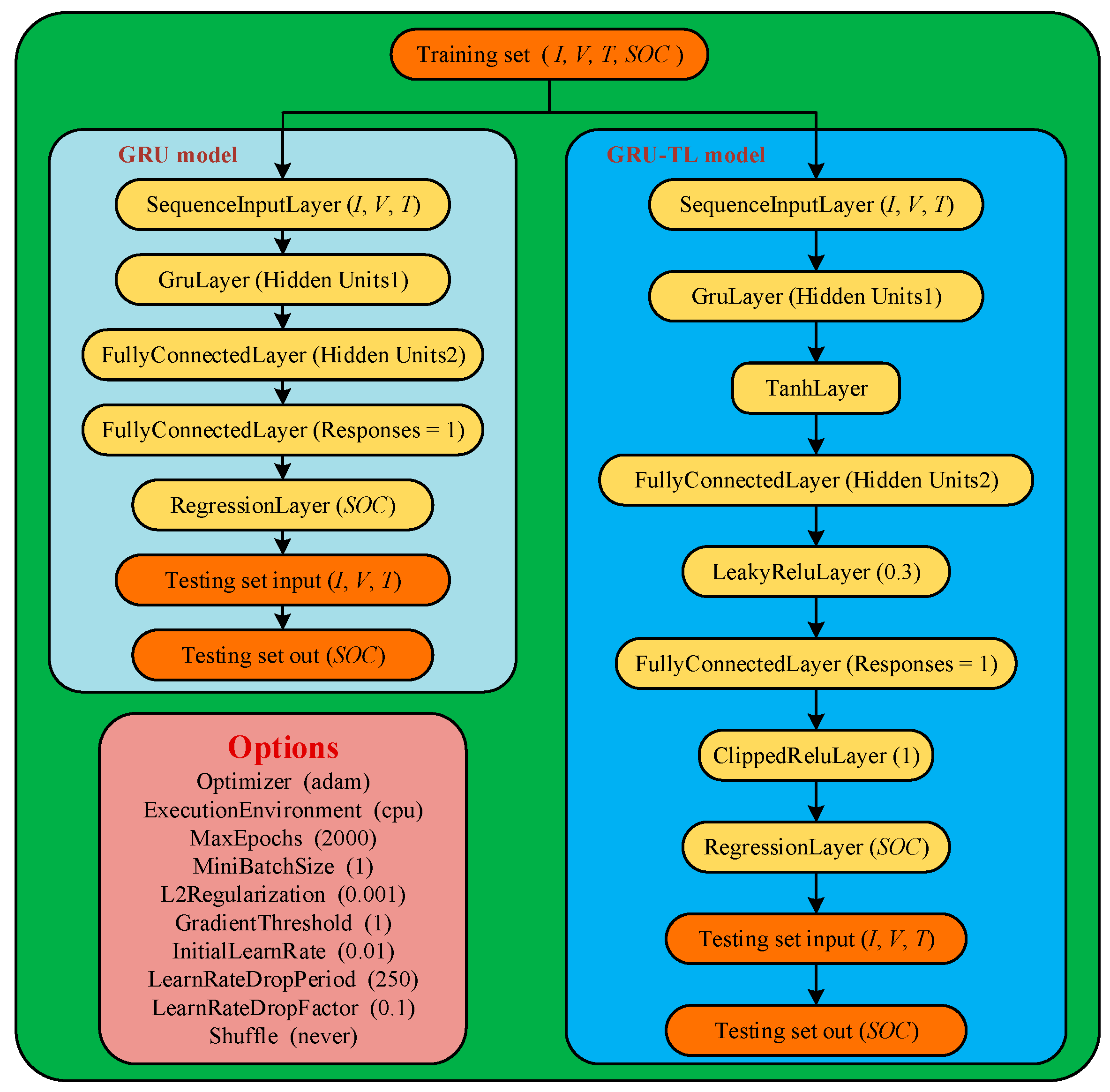
2. GRU-FC Network Model
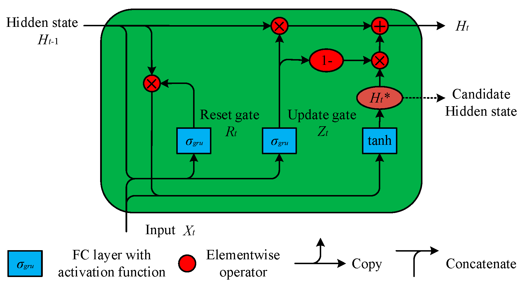
2.1. GRU Structural Unit
2.2. SOC Estimation Based on GRU-ATL Network
2.3. Selection of Other Parameters in Network
3. Battery Data Description and Processing Process
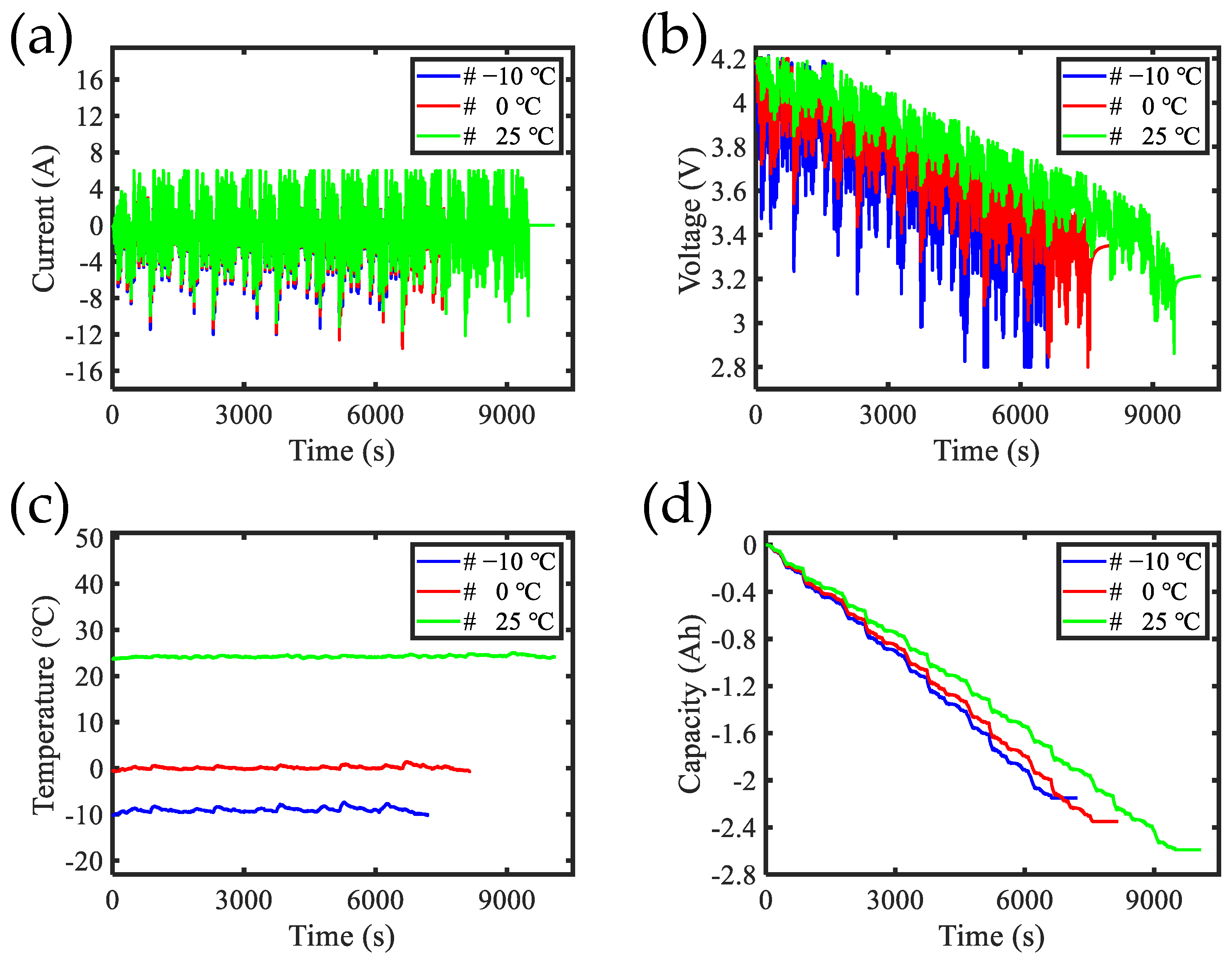
3.1. Battery Data Description
3.2. Data Processing Process and Evaluation Indicators
4. Experimental Results and Discussion
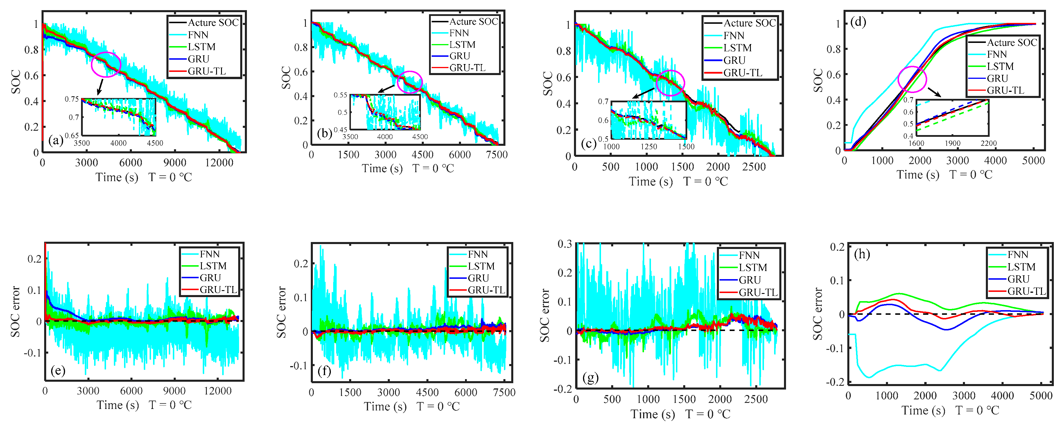
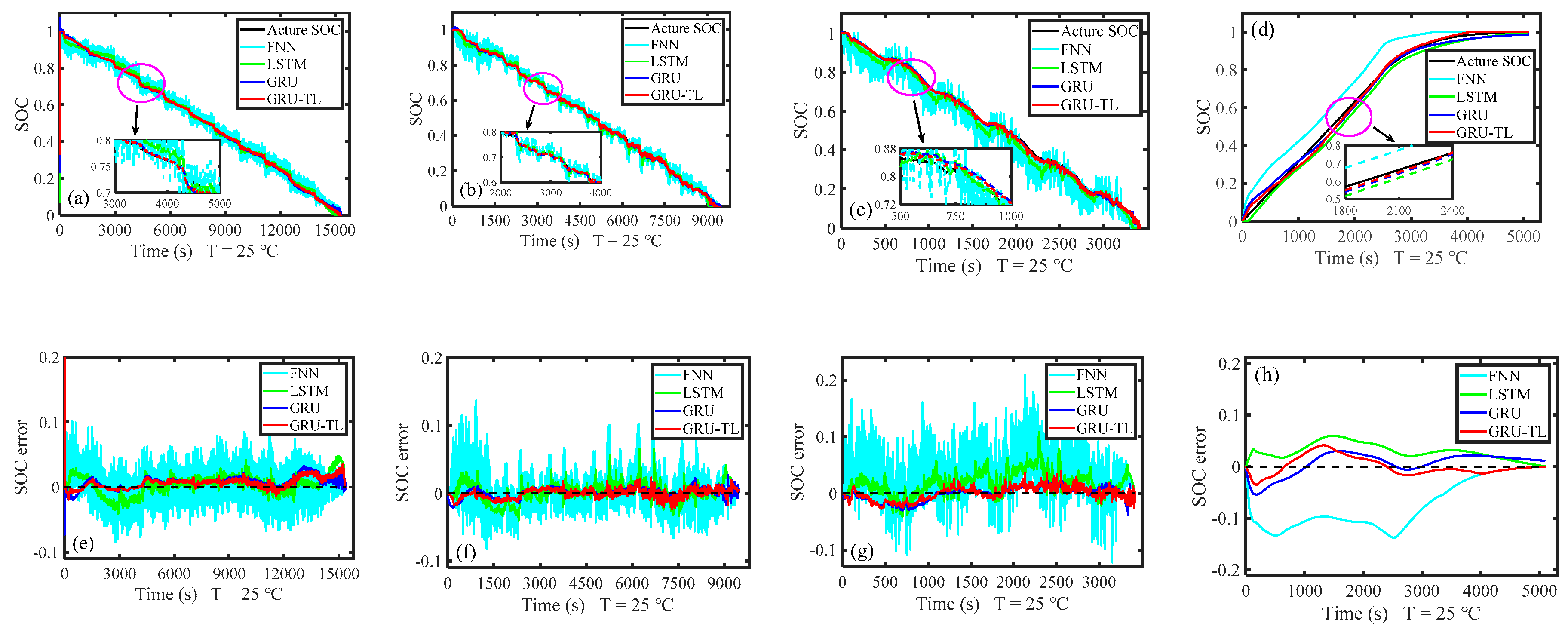
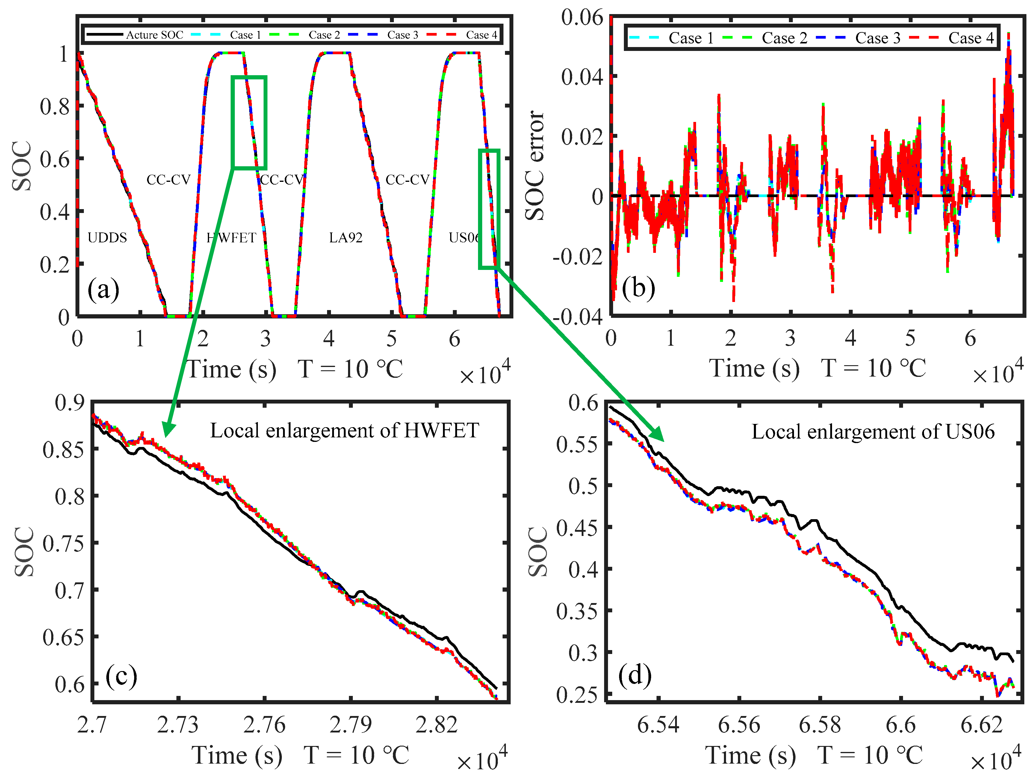
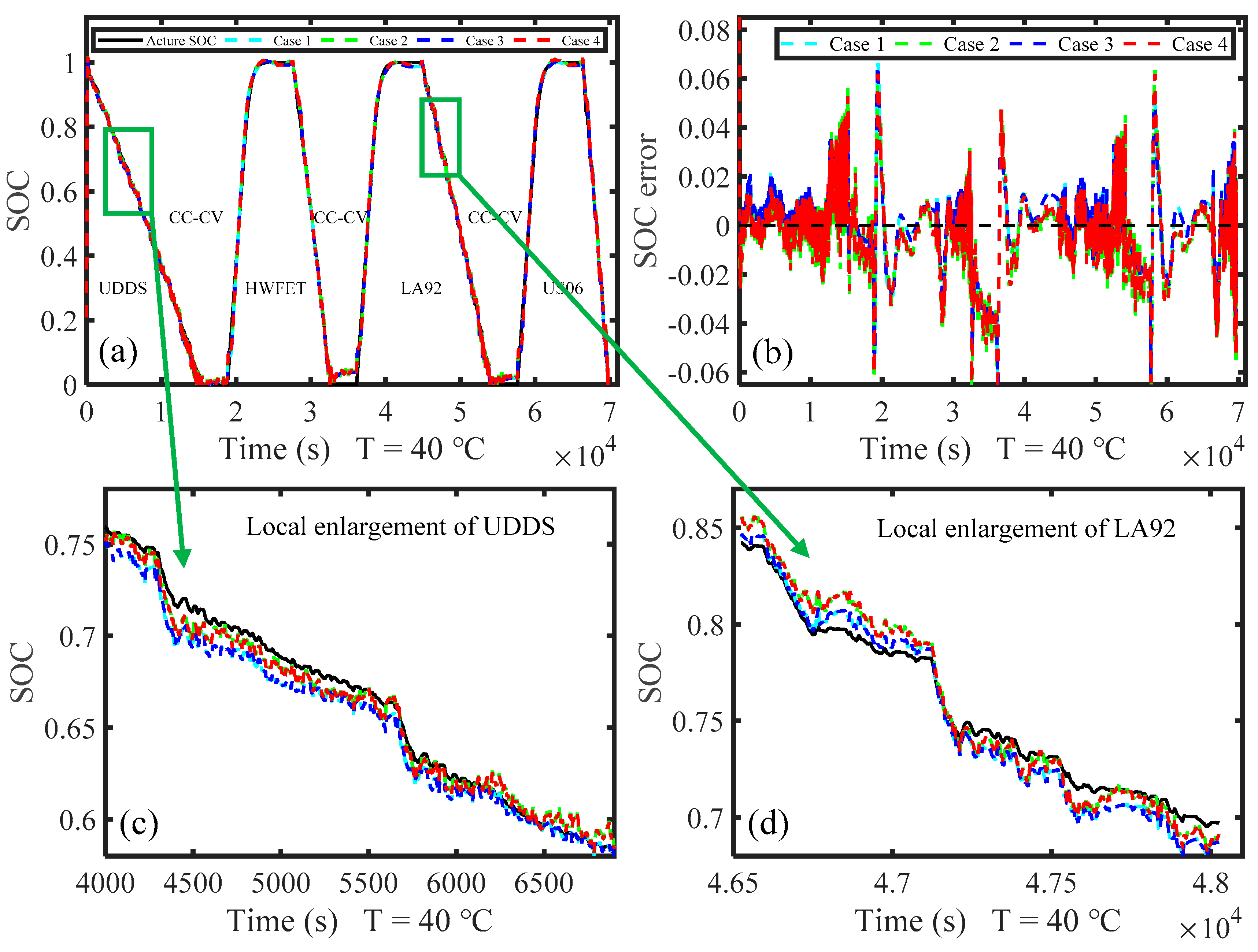
4.1. SOC Estimation Results of Four Network Models
4.2. SOC Estimation Results under Unknown Conditions
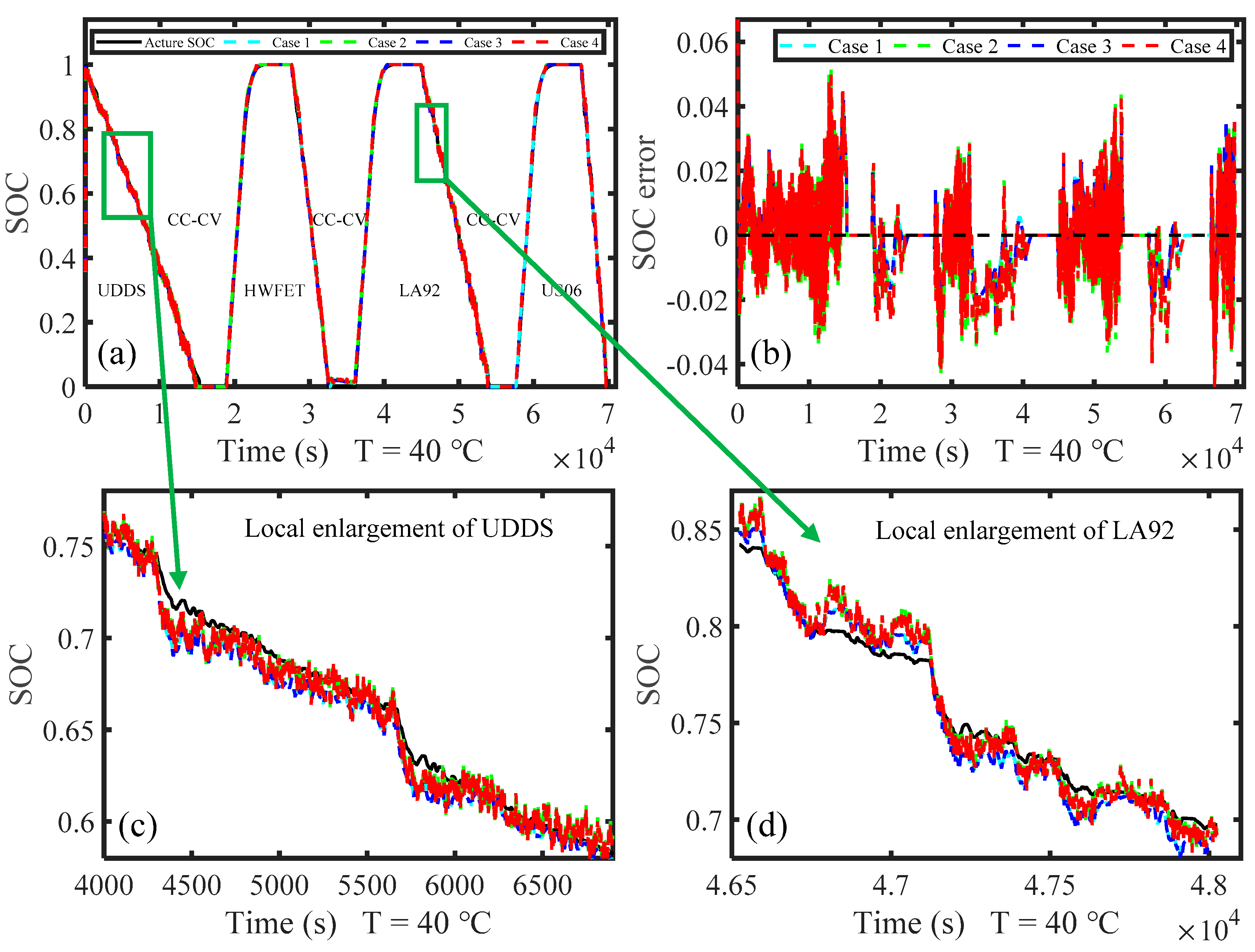
4.3. SOC Estimation Results with Noise
5. Conclusions
- (1)
- Compared with an LSTM network, a GRU network structure has the advantages of fewer parameters and simple structure. It can save a lot of training and prediction time on the premise of ensuring the prediction accuracy of the model. Compared with FNN, LSTM, and GRU network models, it was found that the proposed model could obtain more accurate and stable SOC estimation results in different operating conditions. Adding the above three activation function layers in the GRU-RNN network could improve the prediction accuracy and robustness of the model;
- (2)
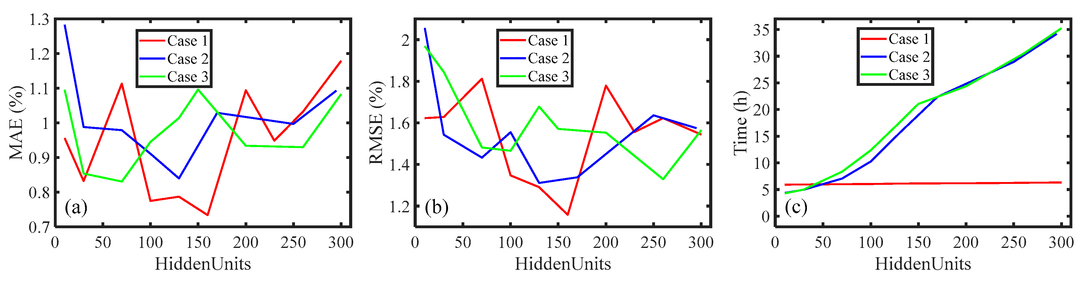
- The prediction accuracy of the model could be improved by appropriately increasing the number of neurons in the GRU layer and FC layer. But the excessive number of neurons in the two layers caused an over fitting phenomenon, which affected the SOC estimation accuracy. In order to save computation, the number of neurons in the GRU layer was 2–3 times less than that in the FC layer. A large number of experiments showed that the SOC was more accurate when the number of neurons in the GRU layer was 55 and that of the FC layer was 160. The MAE was less than 1.3% and RMSE was less than 2%;
- (3)
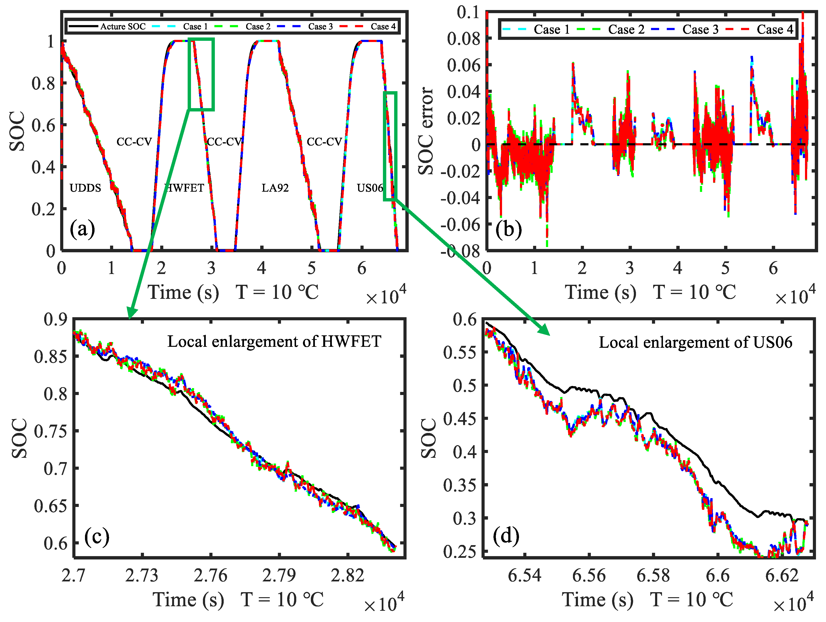
- The SOC prediction performance of LSTM, GRU, and GRU-ATL network models was compared when the measurement signals contained Gaussian noise and non-Gaussian noise. The experimental results showed that the SOC prediction accuracy of GRU-ATL model was 0.1–0.4% higher than the GRU model and 0.3–0.7% higher than the LSTM model. The MAE of SOC predicted by the GRU-ATL model was stable in the range of 0.7–1.4%, and the RMSE was stable between 1.2–1.9%. The SOC prediction results of the GRU-ATL network model were still more accurate and stable at a low temperature;
- (4)
- The experiments in this paper showed that the GRU-ATL network model could realize online SOC estimation under different working conditions without relying on an accurate battery model. When the measurement data contained noise, the model still had high prediction accuracy and robustness, which could meet the SOC estimation in complex vehicle working conditions.
Author Contributions
Funding
Conflicts of Interest
References
- Berecibar, M.; Gandiaga, I.; Villarreal, I.; Omar, N.; Van Mierlo, J.; Van den Bossche, P. Critical review of state of health estimation methods of Li-ion batteries for real applications. Renew. Sustain. Energy Rev. 2016, 56, 572–587. [Google Scholar] [CrossRef]
- Lipu, M.S.H.; Hannan, M.A.; Hussain, A.; Hoque, M.M.; Ker, P.J.; Saad, M.H.M.; Ayob, A. A review of state of health and remaining useful life estimation methods for lithium-ion battery in electric vehicles: Challenges and recommendations. J. Clean. Prod. 2018, 205, 115–133. [Google Scholar] [CrossRef]
- Zhang, C.; He, Y.; Yuan, L.; Xiang, S. Capacity prognostics of lithium-ion batteries using EMD denoising and multiple kernel RVM. IEEE Access 2017, 5, 12061–12070. [Google Scholar] [CrossRef]
- Shrivastava, P.; Soon, T.K.; Idris, M.Y.I.B.; Mekhilef, S. Overview of model-based online state-of-charge estimation using Kalman filter family for lithium-ion batteries. Renew. Sustain. Energy Rev. 2019, 113, 109233. [Google Scholar] [CrossRef]
- Ng, K.S.; Moo, C.; Chen, Y.; Hsieh, Y. Enhanced coulomb counting method for estimating state-of-charge and state-of-health of lithium-ion batteries. Appl. Energy 2009, 86, 1506–1511. [Google Scholar] [CrossRef]
- Petzl, M.; Danzer, M.A. Advancements in OCV Measurement and Analysis for Lithium-Ion Batteries. IEEE Trans. Energy Conver. 2013, 28, 675–681. [Google Scholar] [CrossRef]
- Wang, Q.; Wang, J.; Zhao, P.; Kang, J.; Yan, F.; Du, C. Correlation between the model accuracy and model-based SOC estimation. Electrochim. Acta. 2017, 228, 146–159. [Google Scholar] [CrossRef]
- Li, C.; Xiao, F.; Fan, Y. An approach to state of charge estimation of lithium-ion batteries based on recurrent neural networks with gated recurrent unit. Energies 2019, 12, 1592. [Google Scholar] [CrossRef]
- Yang, F.; Song, X.; Xu, F.; Tsui, K. State-of-charge estimation of lithium-ion batteries via long short-term memory network. IEEE Access 2019, 7, 53792–53799. [Google Scholar] [CrossRef]
- Kim, M.; Chun, H.; Kim, J.; Kim, K.; Yu, J.; Kim, T.; Han, S. Data-efficient parameter identification of electrochemical lithium-ion battery model using deep Bayesian harmony search. Appl. Energy 2019, 254, 113644. [Google Scholar] [CrossRef]
- Bartlett, A.; Marcicki, J.; Onori, S.; Rizzoni, G.; Yang, X.G.; Miller, T. Electrochemical model-based state of charge and capacity estimation for a composite electrode lithium-ion battery. IEEE Trans. Contr. Syst. Technol. 2015, 24, 384–399. [Google Scholar] [CrossRef]
- Xiong, R.; Sun, F.; Chen, Z.; He, H. A data-driven multi-scale extended Kalman filtering based parameter and state estimation approach of lithium-ion polymer battery in electric vehicles. Appl. Energy 2014, 113, 463–476. [Google Scholar] [CrossRef]
- Partovibakhsh, M.; Liu, G. An adaptive unscented kalman filtering approach for online estimation of model parameters and state-of-charge of lithium-ion batteries for autonomous mobile robots. IEEE Trans. Contr. Syst. Technol. 2015, 23, 357–363. [Google Scholar] [CrossRef]
- Wang, S.; Fernandez, C.; Cao, W.; Zou, C.; Yu, C.; Li, X. An adaptive working state iterative calculation method of the power battery by using the improved Kalman filtering algorithm and considering the relaxation effect. J. Power Sources 2019, 428, 67–75. [Google Scholar] [CrossRef]
- Ye, M.; Guo, H.; Cao, B. A model-based adaptive state of charge estimator for a lithium-ion battery using an improved adaptive particle filter. Appl. Energy 2017, 190, 740–748. [Google Scholar] [CrossRef]
- Chen, C.; Xiong, R.; Shen, W. A lithium-ion battery-in-the-loop approach to test and validate multiscale dual h infinity filters for state-of-charge and capacity estimation. IEEE Trans. Power Electron. 2018, 33, 332–342. [Google Scholar] [CrossRef]
- Dai, H.; Xu, T.; Zhu, L.; Wei, X.; Sun, Z. Adaptive model parameter identification for large capacity Li-ion batteries on separated time scales. Appl. Energy 2016, 184, 119–131. [Google Scholar] [CrossRef]
- Yang, H.; Sun, X.; An, Y.; Zhang, X.; Wei, T.; Ma, Y. Online parameters identification and state of charge estimation for lithium-ion capacitor based on improved Cubature Kalman filter. J. Energy Storage 2019, 24, 100810. [Google Scholar] [CrossRef]
- Xia, B.; Sun, Z.; Zhang, R.; Cui, D.; Lao, Z.; Wang, W.; Sun, W.; Lai, Y.; Wang, M. A comparative study of three improved algorithms based on particle filter algorithms in soc estimation of lithium ion batteries. Energies 2017, 10, 1149. [Google Scholar] [CrossRef]
- Fotouhi, A.; Auger, D.J.; Propp, K.; Longo, S. Lithium–sulfur battery state-of-charge observability analysis and estimation. IEEE Trans. Power Electr. 2018, 33, 5847–5859. [Google Scholar] [CrossRef]
- Guo, Y.; Zhao, Z.; Huang, L. Soc estimation of lithium battery based on improved bp neural network. Energy Procedia 2017, 105, 4153–4158. [Google Scholar] [CrossRef]
- Wang, Q.; Wu, P.; Lian, J. SOC estimation algorithm of power lithium battery based on AFSA-BP neural network. J. Eng. 2020, 13, 535–539. [Google Scholar] [CrossRef]
- Chemali, E.; Kollmeyer, P.J.; Preindl, M.; Ahmed, R.; Emadi, A. Long short-term memory networks for accurate state-of-charge estimation of li-ion batteries. IEEE Trans. Ind. Electron. 2018, 65, 6730–6739. [Google Scholar] [CrossRef]
- Bian, C.; He, H.; Yang, S. Stacked bidirectional long short-term memory networks for state-of-charge estimation of lithium-ion batteries. Energy 2020, 191, 116538. [Google Scholar] [CrossRef]
- Vidal, C.; Kollmeyer, P.J.; Naguib, M.; Malysz, P.; Gross, O.; Emadi, A. Robust xev battery state-of-charge estimator design using a feedforward deep neural network. SAE Int. J. Adv. Curr. Prac. Mobil. 2020, 2, 2872–2880. [Google Scholar]
- Yang, F.; Li, W.; Li, C.; Miao, Q. State-of-charge estimation of lithium-ion batteries based on gated recurrent neural network. Energy 2019, 175, 66–75. [Google Scholar] [CrossRef]
- Jiao, M.; Wang, D.; Qiu, J. A GRU-RNN based momentum optimized algorithm for SOC estimation. J. Power Sources 2020, 459, 228051. [Google Scholar] [CrossRef]
- Dong, G.; Zhang, X.; Zhang, C.; Chen, Z. A method for state of energy estimation of lithium-ion batteries based on neural network model. Energy 2015, 90, 879–888. [Google Scholar] [CrossRef]
- Tian, Y.; Lai, R.; Li, X.; Xiang, L.; Tian, J. A combined method for state-of-charge estimation for lithium-ion batteries using a long short-term memory network and an adaptive cubature Kalman filter. Appl. Energy 2020, 265, 114789. [Google Scholar] [CrossRef]
- Cho, K.; Courville, A.; Bengio, Y. Describing Multimedia Content Using Attention-Based Encoder-Decoder Networks. IEEE Trans. Multimed. 2015, 17, 1875–1886. [Google Scholar] [CrossRef]
- Song, Y.; Li, L.; Peng, Y.; Liu, D. Lithium-Ion. Battery Remaining Useful Life Prediction Based on GRU-RNN; IEEE: Piscataway, NJ, USA, 2018; Volume 2018, pp. 317–322. [Google Scholar]
- Zhang, A.; Lipton, Z.C.; Li, M.; Smola, A.J. Dive into Deep Learning. 2020. Available online: https://github.com/d2l-ai/d2l-zh (accessed on 29 November 2020).
- Maas, A.L.; Hannun, A.Y.; Ng, A.Y. Rectifier nonlinearities improve neural network acoustic models. In Proceedings of the 30th International Conference on Machine Learning, Stanford University, Stanford, CA, USA, 17–19 June 2013; p. 3. [Google Scholar]
- Hannun, A.; Case, C.; Casper, J.; Catanzaro, B.; Diamos, G. Deep Speech: Scaling up end-to-end speech recognition. arXiv 2014, arXiv:1412.5567. [Google Scholar]
- Kingma, D.P.; Ba, J. Adam: A method for stochastic optimization. arXiv 2015, arXiv:1412.6980. [Google Scholar]
- Murphy, K.P. Machine Learning: A Probabilistic Perspective; MIT Press: Cambridge, UK, 2012. [Google Scholar]
- Hochreiter, S.; Schmidhuber, J. Long short-term memory. Neural. Comput. 1997, 9, 1735–1780. [Google Scholar] [CrossRef]
- Cho, K.; Van Merriënboer, B.; Gulcehre, C.; Bahdanau, D.; Bougares, F.; Schwenk, H.; Bengio, Y. Learning Phrase Representations using RNN Encoder-Decoder for Statistical Machine Translation. In Proceedings of the EMNLP 2014—2014 Conference on Empirical Methods in Natural Language Processing, Doha, Qutar, 25–29 October 2014; pp. 1724–1734. [Google Scholar]


| Parameter | Value |
|---|---|
| Nominal capacity/voltage | 3.0 Ah/3.6 V |
| Charge and discharge cut-off voltage | 4.2 V/2.5 V |
| Normal end-of-charge current | 50 mA |
| Max continuous discharge current | 20 A |
| Standard charge current | 1.5 A |
| Energy density | 240 Wh/Kg |
| Data Set | T (°C) | Condition |
|---|---|---|
| Training | −10, 0, 10, 25, 40 | Mixed (1–8), CC-CV (3A), UDDS, HWFET, LA92, US06 |
| Testing 1 | −10 | UDDS, HWFET, LA92, US06, CC-CV (3A) |
| Testing 2 | 0 | UDDS, HWFET, LA92, US06, CC-CV (3A) |
| Testing 3 | 10 | UDDS, HWFET, LA92, US06, CC-CV (3A) |
| Testing 4 | 25 | UDDS, LA92, US06, CC-CV (3A) |
| Testing 5 | 40 | UDDS, HWFET, LA92, US06, CC-CV (3A) |
| Network Model | T (°C) | UDDS | LA92 | US06 | CC-CV | ||||
|---|---|---|---|---|---|---|---|---|---|
| MAE (%) | RMSE (%) | MAE (%) | RMSE (%) | MAE (%) | RMSE (%) | MAE (%) | RMSE (%) | ||
| FNN | −10 | 5.303 | 6.489 | 4.869 | 6.594 | 9.066 | 11.899 | 11.479 | 14.352 |
| 0 | 4.041 | 4.821 | 3.437 | 4.507 | 7.519 | 9.632 | 9.475 | 11.597 | |
| 10 | 2.726 | 3.328 | 2.451 | 3.216 | 6.037 | 7.680 | 8.139 | 10.425 | |
| 25 | 1.612 | 2.078 | 1.784 | 2.404 | 4.305 | 5.490 | 7.427 | 8.827 | |
| 40 | 1.517 | 1.920 | 1.615 | 2.105 | 3.363 | 4.289 | 7.808 | 9.438 | |
| LSTM | −10 | 2.067 | 2.993 | 1.658 | 2.085 | 2.265 | 2.77 | 2.075 | 2.822 |
| 0 | 1.256 | 2.471 | 1.271 | 1.613 | 2.216 | 2.834 | 2.868 | 3.313 | |
| 10 | 1.572 | 2.264 | 1.227 | 1.605 | 2.297 | 2.954 | 1.714 | 1.999 | |
| 25 | 1.261 | 2.017 | 1.080 | 1.416 | 2.225 | 2.787 | 2.869 | 3.249 | |
| 40 | 1.327 | 2.103 | 1.164 | 1.489 | 1.870 | 2.286 | 2.068 | 2.389 | |
| GRU | −10 | 0.558 | 0.899 | 0.454 | 0.551 | 1.587 | 1.724 | 3.165 | 4.387 |
| 0 | 1.129 | 2.333 | 0.694 | 0.865 | 1.294 | 1.670 | 1.650 | 2.069 | |
| 10 | 0.702 | 1.314 | 0.461 | 0.554 | 1.474 | 1.842 | 1.409 | 1.901 | |
| 25 | 0.988 | 1.454 | 0.570 | 0.714 | 1.007 | 1.253 | 1.847 | 2.179 | |
| 40 | 0.612 | 1.046 | 0.620 | 0.800 | 0.989 | 1.321 | 1.604 | 2.072 | |
| GRU-ATL | −10 | 0.424 | 0.752 | 0.445 | 0.596 | 1.126 | 1.323 | 2.436 | 3.004 |
| 0 | 0.406 | 1.161 | 0.361 | 0.500 | 1.324 | 1.898 | 1.142 | 1.685 | |
| 10 | 0.457 | 0.859 | 0.638 | 0.765 | 1.429 | 1.730 | 0.799 | 1.066 | |
| 25 | 0.814 | 1.165 | 0.526 | 0.652 | 0.978 | 1.179 | 1.407 | 1.763 | |
| 40 | 0.609 | 0.890 | 0.541 | 0.709 | 0.911 | 1.148 | 1.303 | 1.613 | |
| Case 1 | NFC | 10 | 30 | 70 | 100 | 130 | 160 | 200 | 230 | 260 | 300 |
| MAE (%) | 0.956 | 0.832 | 1.113 | 0.775 | 0.787 | 0.734 | 1.094 | 0.949 | 1.032 | 1.179 | |
| RMSE (%) | 1.623 | 1.628 | 1.812 | 1.347 | 1.291 | 1.158 | 1.779 | 1.556 | 1.623 | 1.544 | |
| Time (h) | 5.92 | 5.95 | 6.01 | 6.03 | 6.13 | 6.15 | 6.18 | 6.21 | 6.26 | 6.33 | |
| Case 2 | NGRU | 10 | 30 | 70 | 100 | 130 | 160 | 200 | 230 | 260 | 295 |
| MAE (%) | 1.283 | 0.988 | 0.979 | 0.911 | 0.840 | 1.029 | NA | 0.997 | NA | 1.093 | |
| RMSE (%) | 2.056 | 1.543 | 1.433 | 1.555 | 1.311 | 1.338 | NA | 1.636 | NA | 1.575 | |
| Time (h) | 4.37 | 4.98 | 7.05 | 10.26 | 15.55 | 22.38 | NA | 28.93 | NA | 34.16 | |
| Case 3 | NGRU and NFC | 10 | 30 | 70 | 100 | 130 | 160 | 200 | 230 | 260 | 300 |
| MAE (%) | 1.095 | 0.854 | 0.831 | 0.945 | 1.014 | 1.096 | 0.934 | NA | 0.930 | 1.083 | |
| RMSE (%) | 1.969 | 1.845 | 1.482 | 1.466 | 1.678 | 1.571 | 1.553 | NA | 1.329 | 1.565 | |
| Time (h) | 4.27 | 5.01 | 8.36 | 12.37 | 17.52 | 21.05 | 24.37 | NA | 30.45 | 35.25 |
| T (°C) | −10 | 0 | 10 | 25 | 40 |
|---|---|---|---|---|---|
| MAE (%) | 1.271 | 0.814 | 1.032 | 0.734 | 0.799 |
| RMSE (%) | 2.005 | 1.101 | 1.461 | 1.158 | 1.259 |
| Network Model | Noise 1 | Noise 3 | ||||||||||
|---|---|---|---|---|---|---|---|---|---|---|---|---|
| T (°C) | −10 | 0 | 10 | 25 | 40 | −10 | 0 | 10 | 25 | 40 | ||
| LSTM | Case 1 | MAE (%) | 1.755 | 1.293 | 1.202 | 1.195 | 1.157 | 1.738 | 1.306 | 1.197 | 1.201 | 1.160 |
| RMSE (%) | 2.369 | 1.879 | 1.695 | 1.751 | 1.689 | 2.358 | 1.894 | 1.693 | 1.754 | 1.691 | ||
| Case 2 | MAE (%) | 1.820 | 1.364 | 1.295 | 1.288 | 1.258 | 1.738 | 1.357 | 1.457 | 1.284 | 1.284 | |
| RMSE (%) | 2.449 | 1.943 | 1.815 | 1.195 | 1.782 | 2.669 | 1.878 | 1.962 | 1.853 | 1.813 | ||
| Case 3 | MAE (%) | 1.756 | 1.301 | 1.206 | 1.198 | 1.161 | 1.750 | 1.317 | 1.210 | 1.201 | 1.168 | |
| RMSE (%) | 2.370 | 1.886 | 1.699 | 1.753 | 1.692 | 2.372 | 1.911 | 1.704 | 1.755 | 1.670 | ||
| Case 4 | MAE (%) | 1.788 | 1.335 | 1.265 | 1.266 | 1.234 | 1.981 | 1.317 | 1.414 | 1.251 | 1.255 | |
| RMSE (%) | 2.410 | 1.915 | 1.780 | 1.815 | 1.759 | 2.572 | 1.850 | 1.913 | 1.823 | 1.786 | ||
| GRU | Case 1 | MAE (%) | 1.687 | 1.277 | 1.169 | 1.272 | 1.010 | 1.687 | 1.295 | 1.165 | 1.281 | 1.015 |
| RMSE (%) | 2.440 | 1.808 | 1.610 | 1.826 | 1.411 | 2.441 | 1.828 | 1.608 | 1.835 | 1.417 | ||
| Case 2 | MAE (%) | 1.697 | 1.299 | 1.180 | 1.305 | 1.113 | 1.687 | 1.160 | 1.410 | 1.250 | 1.062 | |
| RMSE (%) | 2.469 | 1.828 | 1.638 | 1.860 | 1.506 | 2.494 | 1661 | 1.832 | 1.805 | 1.439 | ||
| Case 3 | MAE (%) | 1.692 | 1.278 | 1.169 | 1.272 | 1.011 | 1.700 | 1.297 | 1.168 | 1.273 | 1.019 | |
| RMSE (%) | 2.449 | 1.808 | 1.611 | 1.827 | 1.411 | 2.450 | 1.829 | 1.609 | 1.825 | 1.421 | ||
| Case 4 | MAE (%) | 1.697 | 1.298 | 1.176 | 1.299 | 1.089 | 1.700 | 1.176 | 1.388 | 1.238 | 1.035 | |
| RMSE (%) | 2.473 | 1.826 | 1.634 | 1.853 | 1.479 | 2.473 | 1.679 | 1.810 | 1.795 | 1.411 | ||
| GRU-ATL | Case 1 | MAE (%) | 1.249 | 0.697 | 0.998 | 0.891 | 0.937 | 1.247 | 0.696 | 1.009 | 0.901 | 0.947 |
| RMSE (%) | 1.859 | 1.155 | 1.409 | 1.248 | 1.273 | 1.863 | 1.159 | 1.422 | 1.257 | 1.282 | ||
| Case 2 | MAE (%) | 1.265 | 0.718 | 1.038 | 0.924 | 1.055 | 1.247 | 0.887 | 0.909 | 0.828 | 0.906 | |
| RMSE (%) | 1.888 | 1.171 | 1.45 | 1.288 | 1.413 | 1.865 | 1.235 | 1.278 | 1.197 | 1.275 | ||
| Case 3 | MAE (%) | 1.251 | 0.698 | 1.002 | 0.893 | 0.940 | 1.264 | 0.705 | 1.010 | 0.890 | 0.960 | |
| RMSE (%) | 1.864 | 1.158 | 1.413 | 1.250 | 1.278 | 1.878 | 1.175 | 1.422 | 1.247 | 1.294 | ||
| Case 4 | MAE (%) | 1.268 | 0.722 | 1.040 | 0.928 | 1.042 | 1.359 | 0.855 | 0.910 | 0.828 | 0.893 | |
| RMSE (%) | 1.892 | 1.176 | 1.450 | 1.292 | 1.395 | 1.865 | 1.218 | 1.281 | 1.195 | 1.259 | ||
Publisher’s Note: MDPI stays neutral with regard to jurisdictional claims in published maps and institutional affiliations. |
© 2020 by the authors. Licensee MDPI, Basel, Switzerland. This article is an open access article distributed under the terms and conditions of the Creative Commons Attribution (CC BY) license (http://creativecommons.org/licenses/by/4.0/).
Share and Cite
Duan, W.; Song, C.; Peng, S.; Xiao, F.; Shao, Y.; Song, S. An Improved Gated Recurrent Unit Network Model for State-of-Charge Estimation of Lithium-Ion Battery. Energies 2020, 13, 6366. https://doi.org/10.3390/en13236366
Duan W, Song C, Peng S, Xiao F, Shao Y, Song S. An Improved Gated Recurrent Unit Network Model for State-of-Charge Estimation of Lithium-Ion Battery. Energies. 2020; 13(23):6366. https://doi.org/10.3390/en13236366
Chicago/Turabian StyleDuan, Wenxian, Chuanxue Song, Silun Peng, Feng Xiao, Yulong Shao, and Shixin Song. 2020. "An Improved Gated Recurrent Unit Network Model for State-of-Charge Estimation of Lithium-Ion Battery" Energies 13, no. 23: 6366. https://doi.org/10.3390/en13236366
APA StyleDuan, W., Song, C., Peng, S., Xiao, F., Shao, Y., & Song, S. (2020). An Improved Gated Recurrent Unit Network Model for State-of-Charge Estimation of Lithium-Ion Battery. Energies, 13(23), 6366. https://doi.org/10.3390/en13236366