Modeling the Idaho National Laboratory Thermal-Energy Distribution System (TEDS) in the Modelica Ecosystem

Abstract

Integrated energy systems (IES)—including the intimate coupling between thermal generators, the grid, ancillary processes, and energy storage—are becoming increasingly pertinent to the energy grid. To facilitate a better understanding of IES, Idaho National Laboratory (INL) has developed the experimental Thermal Energy Distribution System (TEDS) to test the interoperability of nuclear reactors, energy storage, and ancillary processes in a real-world setting. This paper provides an overview of the development of TEDS within INL’s Modelica dynamic process modeling ecosystem as part of the IES initiative. The model will bridge the gap between lab-scale experimental results and desired grid-scale energy solutions. Two simulation sets were run. The first was a 5-h test simulating a facility shakedown test, putting the facility through five potential operating modes and showcasing the ability of the valving, control sensors, and component controllers to meet system demands. The second case imposed a typical summer day demand on the system from a region with mixed commercial and residential electrical needs. In this case, the generator alone could not meet peak demand but instead required the thermal-storage unit to act as a peaking unit.

1. Introduction

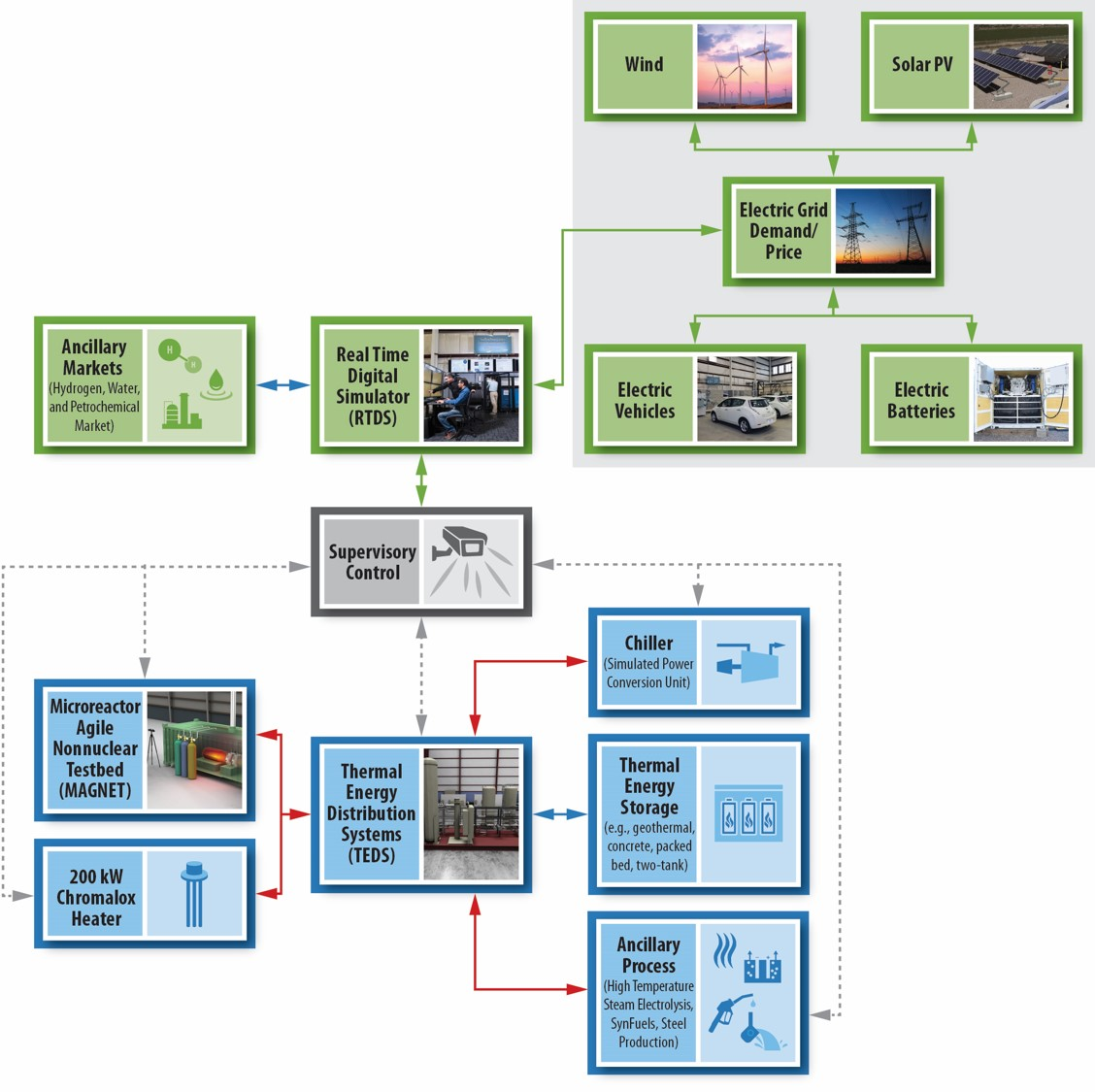
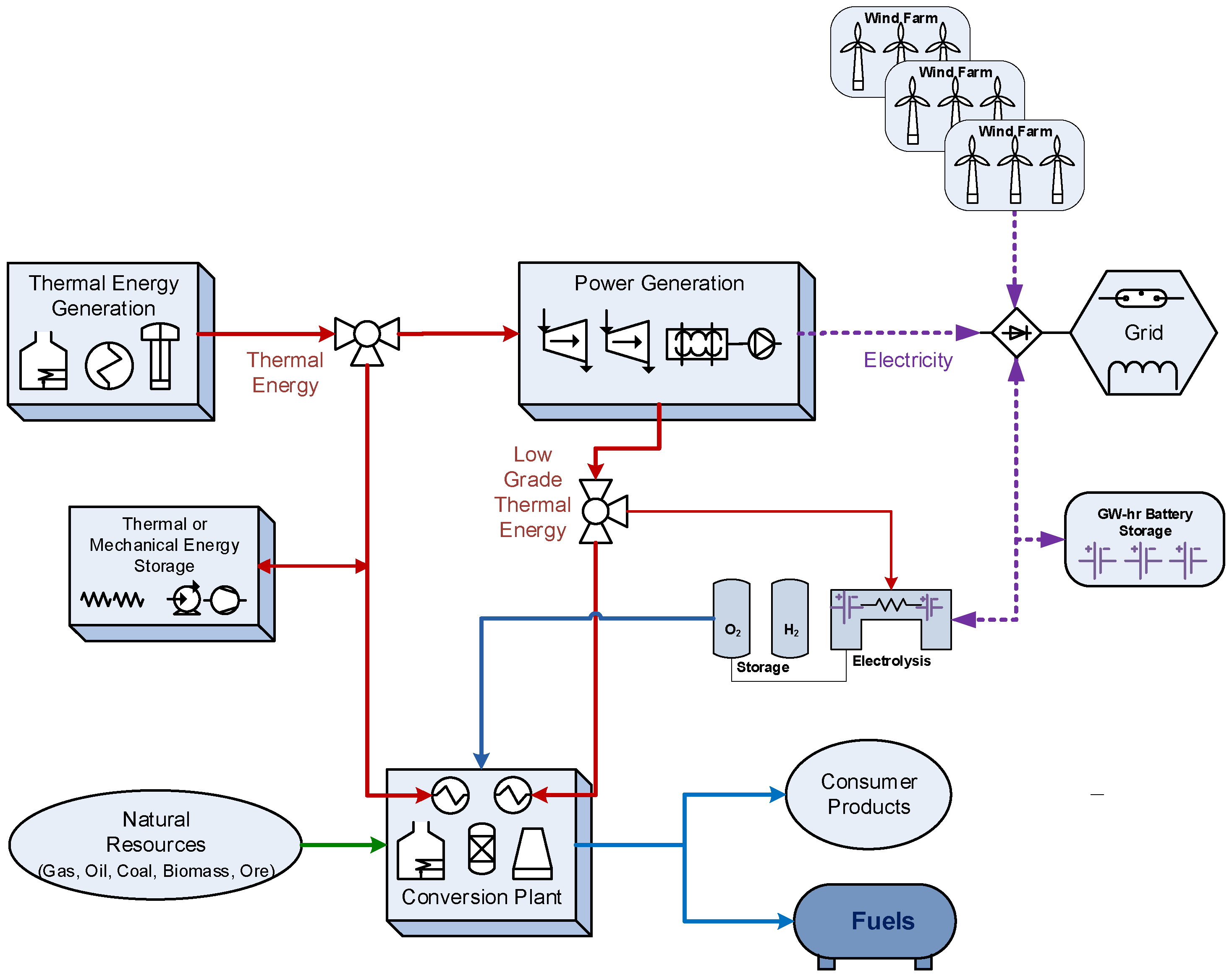
Thermal generators—such as nuclear and coal plants—on the electric grid have traditionally operated in a steady-state base-load mode in which the power level does not change. For these plants, load-follow operation is undesirable due to the associated thermal and mechanical stresses placed on system components. However, variability in grid demand is an inherent part of the modern dynamic lifestyle. Renewable energy sources such as wind and solar introduce variability into the grid supply. As the integration of renewable energy continues, this variability increases, forcing base-load plants to either lose money by supplying unneeded electricity or to load follow. The integrated energy systems (IES) Program, led by Idaho National Laboratory (INL), is researching how to alleviate these economic and physical stressors. IES involves the design, integration, and coordinated operation of various complex, standalone systems. The control algorithms involved are unique to each application and component design. IES architecture can include process steam applications, thermal-energy storage, and intermittent energy sources such as wind and solar (see Figure 1).

The goal of such system integration is to operate as economically and efficiently as possible in simultaneously meeting multiple energy demands. For integrated energy parks that incorporate thermal storage, this means operating thermal generators at full power, storing excess energy for later use during times of low total demand, and discharging that energy during times of high demand [1,2].

To accommodate the vast array of possibilities that integrated energy parks introduce, INL has been developing a library of high-fidelity process models in the Modelica modeling language since early 2013 [3,4]. The Modelica language is a non-proprietary, object-oriented, equation-based language used to conveniently model complex, physical systems. Modelica is an inherently time-dependent modeling language that allows the swift interconnection of independently developed models. Being an equation-based modeling language that employs differential algebraic equation (DAE) solvers, users can focus on the physics of the problem rather than the solving technique, allowing faster model generation and, ultimately, analysis. This feature, alongside model flexibility, has led to the widespread use of the Modelica language across industry for commercial applications. System interconnectivity and the ability to quickly develop novel control strategies while still encompassing overall system physics is why INL has chosen to develop the IES framework in the Modelica language.

Currently available dynamic models include thermal-energy storage (two-tank sensible heat storage; additional models under development), battery-energy storage (logical electrical battery), reverse osmosis, four-loop pressurized-water-reactor nuclear power plants, the NuScale integral pressurized-water reactor, natural gas turbines, coal plants, high-temperature steam electrolysis, and switchyards. The models are a cornerstone of the IES Program at INL. They are used to create and characterize system inertia, thermal losses, and the efficiency of integrated systems. These physical models help map physical performance to economic performance, allowing system-level optimization in regard to both system design and energy dispatch. In addition, these models are used to test innovative system-level control strategies for interconnected thermal generators.

However, due to limited experimental data, the understanding of the interconnection between systems is limited. To help address this shortfall in data and understanding, the Dynamic Energy Transport and Integration Laboratory (DETAIL) is being designed for installation within INL’s Energy Systems Laboratory to demonstrate integrated system operation. The overall objective of the DETAIL facility is to demonstrate simultaneous, coordinated, efficient transient distribution of electricity and heat for power generation, energy storage, and industrial end-uses, with a focus on nuclear systems. The combined DETAIL facility, which incorporates electrically heated systems to emulate thermal-energy input from a nuclear reactor, will demonstrate real-time integration of the electrical grid, renewable energy inputs, thermal- and electrical-energy storage, and energy delivery to the end user. Such simulation of an integrated energy network can improve our ability to optimize energy flows while maintaining system stability and efficient operation of all system assets.

The Thermal Energy Distribution System (TEDS), shown in Figure 2, acts as the backbone of the DETAIL facility to test heat-transfer components, distribution systems, instruments, and controls that can be monitored and controlled for hybrid generation of electrical power and/or non-electrical products. As is the case for other subsystems within DETAIL, TEDS is designed to operate either independently or as a part of an integrated system. Within the integrated system, TEDS will be connected to the INL Real-Time Power Simulation test platform to develop and demonstrate monitoring/control systems and investigate real-time, hardware-in-the-loop response characteristics relative to grid operations. The system can characterize thermal-energy inertia and management relative to the interoperability of power generation, energy storage, and industrial heat applications. Furthermore, TEDS will provide data to validate computational models such as RELAP, Modelica, and other transient-physics-based models in support of the scaling up of hybrid energy systems to be demonstrated with operating (fueled) nuclear plants. TEDS can also support cyber-informed engineering of controls and hardware systems.

To model control algorithms and elucidate potential problem areas, a TEDS model based on initial design data was developed in Modelica. This model was implemented using the commercially available Modelica-based modeling and simulation environment (Dynamic Modeling Laboratory (Dymola) version 2021) [5]. In-house-developed packages and open-source libraries facilitated the modeling and simulation. In particular, the Modelica Standard Library version 3.2.3 [6] and TRANSFORM [7] from Oak Ridge National Laboratory (ORNL) were employed.

Through the creation of a TEDS model and experimental facility, research organizations and industry will be able to demonstrate and test technologies within an experimental facility both digitally and experimentally. In the initial stages, researchers will be able to leverage the existing TEDS Modelica model to test any number of new and unique control strategies, coupling mechanisms, ancillary processes, system sizing, and system response to various externalities, such as market conditions. Researchers and industry partners will then be able to bring their technology into the lab to verify their selected computational permutation and obtain data for validation and verification and licensing purposes. This report provides an in-depth view of the Modelica model that will act as an informant to the experimental team prior to final installation and deployment, later serving as a verification and validation benchmark and modeling tool for the rest of the IES modeling and outreach efforts.

2. Components and Subsystems

TEDS involves the combination of several components and subsystems working in unison via control algorithms to ensure the proper transport of thermal energy throughout the system [8]. These subsystems and components include a single-tank packed-bed thermocline energy storage subsystem; a programmable Chromalox heater designed to simulate a thermal generator unit offtake, such as nuclear reactor secondary-side bypass steam; an ethylene glycol heat exchanger; three materials to transfer heat throughout the system (therminol-66, ethylene glycol, and alumina beads); and a series of FOAMGLAS^® ONE insulated pipes to ensure proper flow redirection and heat conservation. Additionally, TEDS has several unused flange connections that are intended for future connection with ancillary processes, allowing demonstration of interconnection hardware and complex control systems necessary to distribute energy to multiple processes in parallel.

2.1. Thermocline

A major component of the initial TEDS configuration is the single-tank packed-bed thermocline system. This thermal-energy storage component can store 200 kWht of thermal energy. A thermocline storage system stores heat via a singular hot and cold fluid separated by a thin thermocline region occurring due to the density differential between the fluid at different temperatures. Assuming low mixing via internal flow characteristics and structural design, this thermocline region can be kept relatively small compared to the size of the tank. Additionally, low internal thermal conductivity and large changes in buoyancy are extremely useful in maintaining a small relative thermocline thickness.

To increase the cost-effectiveness of these designs, it is common to fill the tank with a low-cost filler material such as concrete or quartzite. These filler materials are inexpensive, have high density, and high thermal conductivity. By using such material, a reduction in the amount of high cost thermal fluid can be achieved, thereby increasing the economic competitiveness of such designs.

2.1.1. Thermocline Model

The thermocline system was modeled using a modified set of Schumann equations originally introduced in 1927 [9]. The equation set governs the energy conservation of fluid flow through porous media. It has been widely adopted in analyzing thermocline storage tanks. The modified equation set adopted a new version of the convective heat-transfer coefficient, pioneered by Gunn in 1978 [10], in order to incorporate low- and no-flow conditions. Additionally, a conductive heat-transfer term was added to account for heat conduction through the tank walls. Self-degradation of the thermocline in the axial direction is neglected due to the low relative values during standard operation; this is a known limit of the model during times of no flow.

Energy balance for the fluid

$$a_f=\epsilon \pi R^2$$

where $a_f$ is the cross-sectional area of the fluid, $\epsilon$ is porosity of the tank, and R is radius of the tank.

$${\rho }_f\epsilon \pi R^{2}U\left(h_z-h_{z+dz}\right)+h_c{S}_r\left(T_r-T_f\right)dz+{\dot{Q}}_{losses}={\rho }_f{C}_f\epsilon \pi R^{2}dz\frac{\partial T_f}{\partial t}$$

where $h_z$ is the enthalpy at node i, ${\dot{Q}}_{losses}$ is heat conduction through the walls, $T_f$ is the temperature of the fluid at node i, $T_r$ is the filler temperature at node i, and $C_f$ is the heat capacity of the fluid.

$$U=\frac{\dot{m}}{{\rho }_f{a}_f}$$

where $\dot{m}$ is the fluid mass flow $\dot{m}>0$ is fluid moving from the hot side to the cold side,$\dot{m}<0$ is fluid moving from the cold side to the hot side. ${\rho }_f$ is the fluid density at node i, and $U$ is the fluid velocity.

$$S_r=\frac{f_s\pi R^2\left(1-\epsilon \right)}{r_{filler}}$$

$S_r$is the heat-transfer area of filler per unit length of the tank, $f_s$ is the surface shape factor, and $r_{filler}$ is the radius of filler beads.

$$h_c=\left(\left(7-10\epsilon +5{\epsilon }^2\right)\left(1+0.7R{e}^{0.2}P{r}^{0.33}\right)+\left(1.33-2.4\epsilon +1.2{\epsilon }^2\right)R{e}^{0.7}P{r}^{0.33}\right)\frac{k_{fluid}}{2r_{char}}$$

$$Re=\frac{4r_{char}\dot{m}}{a_f{\mu }_f}$$

$$r_{char}=\frac{\epsilon d_r}{4\left(1-\epsilon \right)}$$

$h_c$ is the convective heat transfer coefficient, $r_{char}$is the characteristic radius, and $d_r$is the diameter of the filler material.

Energy balance for the filler material

$$h_c{S}_r\left(T_r-T_f\right)dz=-{\rho }_r{C}_r\left(1-\epsilon \right)\pi R^{2}dz\frac{\partial T_r}{\partial t}$$

The above equation is the filler material energy balance where $C_r$ is the heat capacity of the filler and ${\rho }_r$ is the filler density.

2.1.2. Thermocline Nodalization

The thermocline system is split into axial nodes that each incorporate a fluid and a solid component. During charging, the flow runs from the hot side to the cold side; it runs in the opposite direction during discharge. Boundary conditions for each node depend on the direction of the flow and the advection of the previous node’s values. For example, if the thermocline is operating in discharge mode, node N − 1 will receive boundary values from node N − 2. Whereas, if in charging mode, node N − 1 will use boundary conditions from node N. Figure 3 provides a representation of this nodal split.

In addition to the axial representation of the heat distribution winthin a packed-bed porous medium, one must consider radial heat loss through the tank walls and insulation surrounding the tank and in the ambient surroundings. To account for this, the simulation calculates heat loss from the tank in each nodal fluid profile. Heat loss is calculated via Fourier’s law of heat conduction ($q^{″}=-k\frac{dT}{dx}$) using built-in Modelica conduction models for cylinders. This heat loss is then spread out over the entire fluid volume at each axial position, interacting with the solid volume through standard convection in the energy balance for the filler.

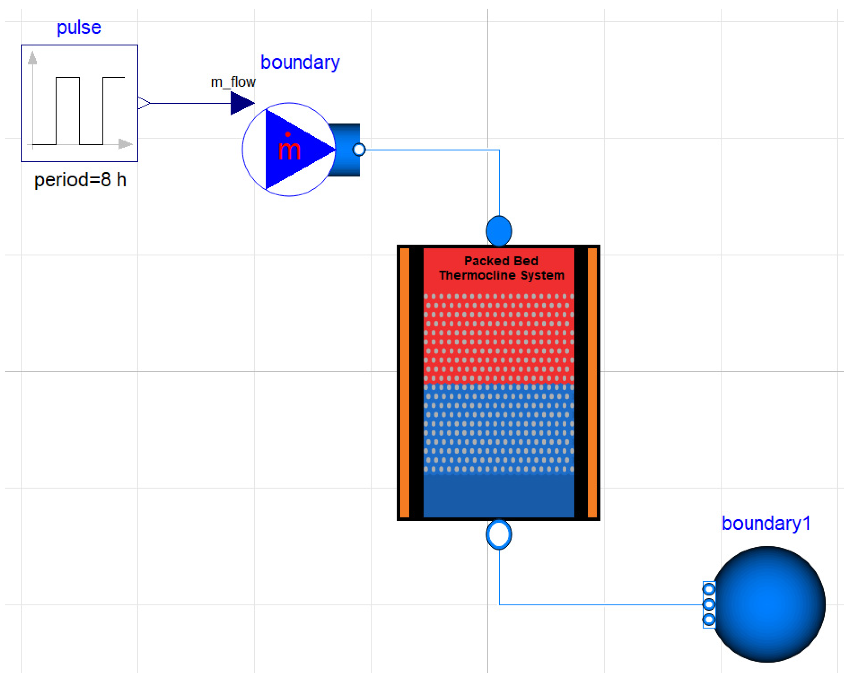
2.1.3. Thermocline Test Case

To demonstrate the ability of the model to properly charge and discharge through hourly and daily cycling, a periodic test was conducted. The system parameters are given in

Table 1. Test case parameters.

Parameter	Value
Fluid Material	Therminol-66
Filler Material	Alumina
Wall Material	Stainless Steel
Insulation Material	Fiberglass
Porosity	0.6
Tank Height	14.6 m
Tank Radius	7.6 m
Ambient Temperature	20 °C
Nodes	200
Wall Thickness	0.051 m
Insulation Thickness	0.204 m
Charge Incoming Temperature	325 °C
Discharge Incoming Temperature	225 °C

. Therminol-66 is the working fluid, and the filler material is alumina beads with a total porosity of 0.6, meaning that the system is 40% alumina beads by volume. To test the charging and discharging capability, an 8 h periodic cycle was imposed on the system. The first four hours were spent discharging the system, and the next four were spent charging the system with hot therminol-66. 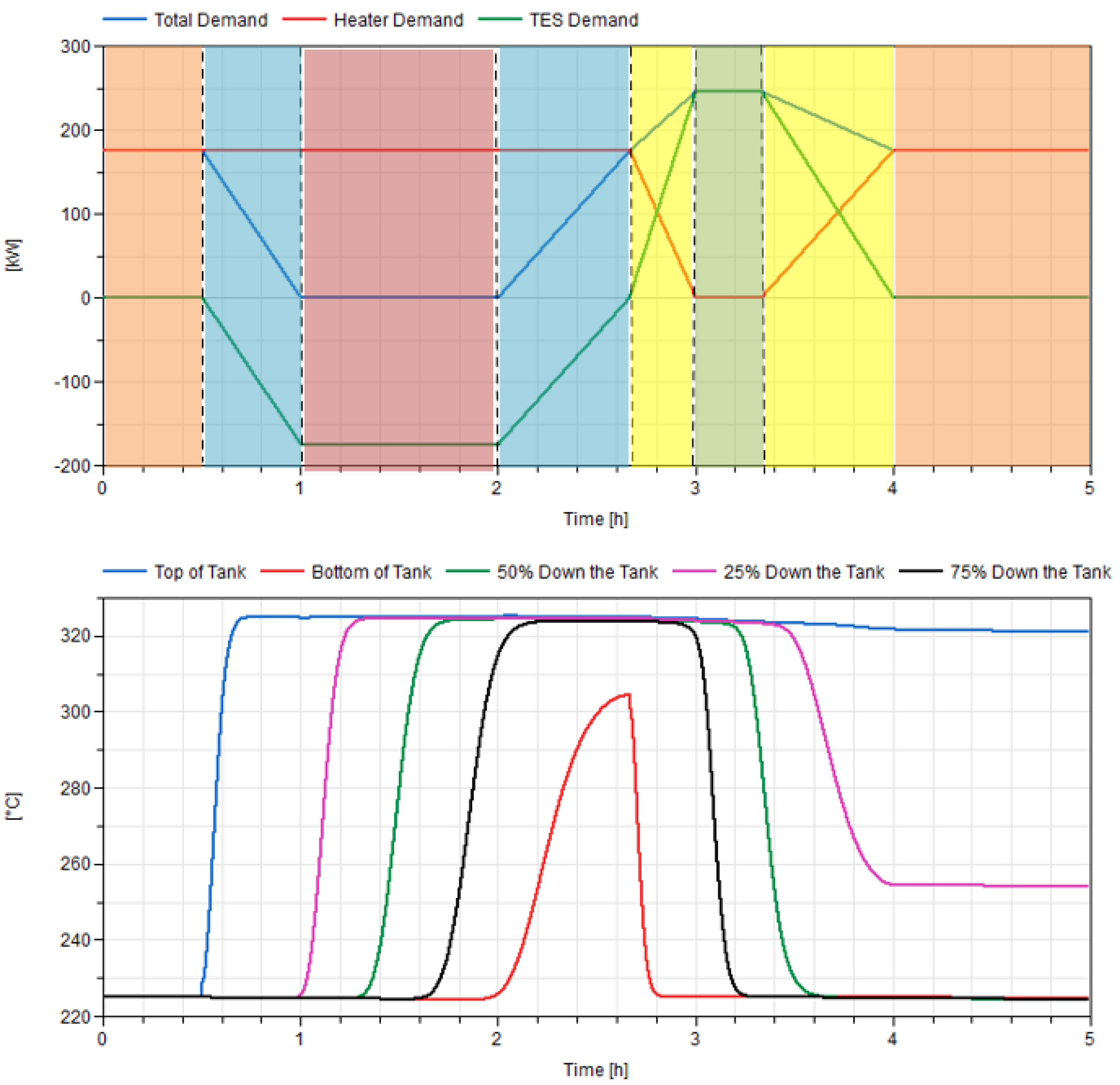This is illustrated in Figure 4. Figure 5 shows that the bottom of the tank quickly falls in temperature as the colder fluid enters during the discharge operation and starts moving up the tank. Toward the end of the initial four hours, the top of the thermocline tank begins to decrease in temperature as the thermal gradient reaches the top of the tank. At this point, the thermocline is no longer a useful source of heat. Then, at Hour 4, the flow reverses, and the tank begins to charge with hot fluid. As the hot fluid charges from the top—as opposed to entering from the bottom of the tank—the top node of i = 1 returns to 325 °C as the hot fluid passes that position and moves down the tank. Initially, the bottom of the tank remains at the nominal value of 225 °C. However, toward the end of Hour 4, the bottom of the tank begins to increase in temperature as the thermal gradient reaches it, at which point the tank is almost fully charged. The filler material follows the same pattern in each node, as depicted at the bottom of Figure 5. These transient simulations were repeated over the next 50+ h with unvarying results due to the tank being well-insulated by 0.2 m of fiberglass, despite the large ambient-temperature difference. The filler material, though a large source of stored heat per volume, exacerbates the thermocline, as it conducts heat to the fluid. This can be seen at hour 8, when node 150 has not yet reached the nominal inlet temperature but node 200 is already being heated. This means that, at that point, the bottom quarter of the tank is a thermal gradient due to the time lag in the filler giving up its heat as the thermocline passes.

2.2. Materials

To correctly model the system, several new materials had to be implemented in Modelica: therminol-66, ethylene glycol, alumina, and FOAMGLAS^® ONE (insulation). Operational limits for therminol-66 and ethylene glycol are shown in

Table 2. Fluid operational limits at 1 atm.

Material	Boiling Point	Operational Band
Therminol-66	358 °C (678 °F)	−2.7–343.3 °C (27–650 °F)
Ethylene Glycol (50% by vol.)	~110 °C (230 °F)	−30–105 °C (−22–221 °F)

.

To maintain library consistency, each of these materials was added to the TRANSFORM library housed at ORNL, under their pre-existing media package.

2.2.1. Therminol-66

Therminol-66 is a heat-transfer fluid sold by Solutia (Eastman Chemical Company) and used for decades in the chemical industry for heat-transfer applications. Therminol-66′s properties in Modelica are as follows [11]:

$$\rho \left(T\right)\left[\frac{\mathrm{kg}}{{\mathrm{m}}^3}\right]=-0.000321T^2-0.614254T+1020.62;T\mathrm{in}\mathrm{Celsius}$$

$$\mu \left(T\right)\left[\mathrm{Pa}\ast \mathrm{s}\right]=\rho \left(T\right)\ast \exp \left(\frac{586.375}{T+62.5}-62.5\right)\times {10}^{-6};T\mathrm{in}\mathrm{Celsius}$$

$$k\left(T\right)\left[\frac{\mathrm{W}}{\mathrm{m}\ast \mathrm{K}}\right]=-0.00000015T^2-0.000033T+0.118294;T\mathrm{in}\mathrm{Celsius}$$

$$c_p\left(T\right)\left[\frac{\mathrm{kJ}}{\mathrm{kg}\ast \mathrm{K}}\right]=0.0000008970785T^2+0.003313T+1.496005;T\mathrm{in}\mathrm{Celsius}$$

In determining the properties of therminol-66, specific heat is calculated once at the average planned operational temperature and assumed constant over that band in respect to temperature. This assumption greatly reduces the property solutions used in Modelica, as it avoids many derivative calculations in the continuous space. This assumption is reasonable if one chooses the average operational fluid temperature, and specific heat can be assumed to be linear over that span. All other properties are continuously updated.

2.2.2. Ethylene Glycol (50% Water by vol.)

Ethylene glycol’s properties are as follows:

$$\rho \left(T\right)\left[\frac{\mathrm{kg}}{{\mathrm{m}}^3}\right]=-0.002435T^2-0.338484T+1082.287;T\mathrm{in}\mathrm{Celsius}$$

$$\mu \left(T\right)\left[\mathrm{Pa}\ast \mathrm{s}\right]=-0.00001474T^3+0.00474114T^2-0.50420746T+20.088\times {10}^{-3};T\mathrm{in}\mathrm{Celsius}$$

$$k\left(T\right)\left[\frac{\mathrm{W}}{\mathrm{m}\ast \mathrm{K}}\right]=\left(8.9758T\times {10}^{-5}-1.3975T^2\times {10}^{-6}+0.23951\right)\ast 1.729577;T\mathrm{in}\mathrm{Celsius}$$

$$c_p\left(T\right)\left[\frac{\mathrm{J}}{\mathrm{kg}\ast \mathrm{K}}\right]=\left(7.3219T\times {10}^{-4}+0.81485\right)\ast 4180;T\mathrm{in}\mathrm{Celsius}$$

As with therminol-66, specific heat is calculated once at the average planned operational temperature and assumed constant over that band in respect to temperature. All other fluid properties are continuously updated. Ethylene glycol’s properties are taken from a mixture of sources [12,13]. Ethylene glycol used in the heat exchanger is assumed to be 50% water by volume and the above properties are consistent with this assumption.

2.2.3. Alumina (Al₂O₃)

Alumina’s properties are as follows, based upon [14]:

$$\rho \left(T\right)\left[\frac{\mathrm{kg}}{{\mathrm{m}}^3}\right]=3950$$

$$k\left(T\right)\left[\frac{\mathrm{W}}{\mathrm{m}\ast \mathrm{K}}\right]=5.85+15360\exp \left(\frac{-0.002T}{T+516}\right);T\mathrm{in}\mathrm{Celsius}$$

$$c_p\left(T\right)\left[\frac{\mathrm{J}}{\mathrm{kg}\ast \mathrm{K}}\right]=1117+0.14T-411\exp \left(-0.006T\right);T\mathrm{in}\mathrm{Celsius}$$

The material properties were thoroughly tested inside the Modelica framework to ensure matching values with the literature.

2.2.4. FOAMGLAS^® ONE

FOAMGLAS^® ONE properties for the insulating material are taken from [15].

$$\rho \left(T\right)\left[\frac{\mathrm{kg}}{{\mathrm{m}}^3}\right]=117$$

$$k\left(T\right)\left[\frac{\mathrm{W}}{\mathrm{m}\ast \mathrm{K}}\right]=2.59916\times {10}^{-7}{T}^2+1.40496\times {10}^{-4}T+0.0384688;T\mathrm{in}\mathrm{Celsius}$$

$$c_p\left(T\right)\left[\frac{\mathrm{J}}{\mathrm{kg}\ast \mathrm{K}}\right]=770$$

2.3. Chromalox Heater

The Chromalox heater was modeled as a multi-node pipe with the heat input equally distributed throughout, as shown in Figure 6. The heater operates to maintain the temperature at “sensor_T1” at some nominal setpoint. This is controlled via a proportional integral derivative (PID) controller that ensures equal heat input into each segment of the Chromalox heater. The heater is bounded to a maximum heater input according to vendor specifications. For pressure loss calculations, heater mass flow is assumed to be fully developed and capable of operating in either the laminar or turbulent region, depending on the pipe’s Reynolds number. Heat transfer into the pipe is assumed to be ideal, since the heating elements are in direct contact with the fluid.

2.4. Ethylene Glycol Heat Exchanger

The ethylene glycol heat exchanger was modeled using the TRANSFORM heat exchanger model as a shell and tube heat exchanger, with therminol-66 operating on the shell side of the heat exchanger and ethylene glycol on the tube side. The ethylene glycol flow rate operates via a flow control valve that helps ensure that the therminol-66 comes out of the heat exchanger at a specified temperature setpoint. Tube material for the heat exchanger can be changed via a drop-down menu but has been specified as stainless steel 316 for TEDS. Heat transfer on the tube side is calculated via the Dittus–Boelter correlation, while heat transfer on the shell side is calculated via single-phase two-region heat transfer in which the correction factors are adjusted to meet predetermined heat-transfer characteristics. The heat exchanger setup is depicted in Figure 7.

2.5. Insulation Thickness

Assuming an infinitely wide tank, perfect insulation, or ambient temperatures equivalent to thermocline tank temperatures, heat loss through the walls of the tank would be ideal. Unfortunately, such conditions do not exist, and heat loss is a constant battle in thermal-storage units. They are of even higher consequence in structures that present a high relative surface area compared to internal volume. Due to size constraints within the experimental lab facility, this is an ever-present reality of the TEDS thermocline tank. Commercial entities that use thermocline tanks for chilled water storage employ tanks with large diameters relative to their heights in order to maintain low thermal losses. However, TEDS has a large surface area relative to its volume, and a large temperature differential between its internal fluid and ambient surroundings. Therefore, determining the necessary insulation thickness comprises a trade-off among price, the physical space to place the insulation, and heat loss. To determine an acceptable level of relative heat loss, a temperature drop-off over a 2-day inactive period (such as a weekend) was simulated. The results are presented in Figure 8.

The simulation assumed an initial thermocline temperature of 325 °C, consistent with a fully charged thermocline system. The flow was assumed to be stagnant. The simulation considered FOAMGLAS^® ONE insulation thicknesses of 0.051 m (2 in.), 0.102 m (4 in.), 0.152 m (6 in.), and 0.203 m (8 in.), with it being known that 0.203 m (8 in.) was the upper bound of physical space surrounding the thermocline in which insulation could be placed. For the 0.051 m (2 in.)-thick insulation, ambient heat loss would equate to an ~80 °C drop in average tank temperature over two days. Four-inch-thick insulation would equate to a 47 °C drop in average temperature, while a 6 in.-thick layer would equate to a 33 °C heat loss. Eight-inch-thick insulation is only modestly better, with a predicted 27 °C drop over two days. From this simulation, it was determined that a 6 in. layer of insulation would be the best trade-off in terms of effective heat storage while adequately fitting within the available space surrounding the tank.

3. TEDS Control Systems

In addition to the components discussed in the previous section, a series of valves, sensors, and control algorithms is required to ensure that all operating modes are possible while still maintaining component properties within acceptable operational limits. A full schematic of the TEDS operational system in Modelica can be seen in Figure 9 and Figure 10. This section seeks to provide an in-depth description of the operational control schemes utilized in TEDS. For purposes of initial deployment, it is assumed that the energy system consists of a heat generator, a thermal-storage unit, and a heat sink (either a standard balance of plant or an ancillary process).

3.1. Operational Modes

The dynamic flexibility of the TEDS project is an inherent by-product of its potential to operate in several different modes. However, with increased flexibility comes increased complexity of controls. To control the system, all foreseeable operating modes must be accommodated within a single cohesive control strategy. The initial deployment configuration features five possible operating modes, each involving the thermal-storage unit (see

Table 3. Foreseeable operating modes.

Mode	Heat Source to Load	Charging (Heat Source to Thermocline)	Discharging (Thermocline to Load)
1	Yes	No	No
2	No	Yes	No
3	No	No	Yes
4	Yes	Yes	No
5	Yes	No	Yes

).

Mode 1 simulates the heat-generation source in standard operating mode with zero-energy storage. This mode is akin to when currently operating generators accommodate a standard load-following mode. Mode 2 simulates a full-charging scenario in which the thermal generator sends all its heat to the thermal-storage unit. Mode 3 simulates a full-discharge scenario. For this mode, the thermal generator is turned off, and the thermal-storage unit is the sole unit providing heat to the balance of plant or ancillary process. Mode 3 simulates scenarios involving reactor trips or brief shutdowns, allowing the grid to bring additional peaking units online. Mode 4 is a combination of Modes 1 and 2, with the thermal generator providing a portion of its heat to thermal storage and another portion to the heat load. Typically, this operational unit provides heat to the load first, then dumps excess heat into the thermal-storage unit for later use. Mode 5 involves a combination of Modes 1 and 3, with both the thermal generator and thermal-storage tank providing heat to the load. This operational modality is common in geographical areas that utilize large amounts of variable renewable energy, such as places in the Midwest that rely heavily on wind energy. To appropriately accommodate these operating modes, a combination of five valves is needed.

Table 4. Valve positioning in TEDS.

Name	Valve	Position (Mode 1)	Position (Mode 2)	Position (Mode 3)	Position (Mode 4)	Position (Mode 5)
GBV-201	1	Closed	Open	Closed	Open	Closed
GBV-006	2	Open	Closed	Closed	Open	Open
GBV-202	3	Closed	Closed	Open	Closed	Open
BV-204	4	Closed	Open	Closed	Open	Closed
GBV-203	5	Closed	Closed	Open	Closed	Open

illustrates each valve’s position in each mode. Notably, six valves appear in Figure 9 and Figure 10; however, GBV-004 (Valve 6) is anticipated for future operations and will remain fully open throughout all the currently presented TEDS testing modalities. It is noted that the flexibility of Modelica’s drag and drop interface allows the researcher to alter these control strategies for a particular system design they are interested in evaluating. This flexibility allows external users the ease to evaluate several control strategies for a system operating within various markets in a very short time, without initially needing to log experimental hours at a facility.

Four of the five valves are strictly required to be fully controllable globe valves, while two can operate as ball valves. In practice, the experimental team made four of the valves globe valves in anticipation of future operational modalities.

3.2. Supervisory Control Scheme

While the ability exists to impose custom demand signals to each individual system component, it is important to consider market scenarios that would initiate each of the modes designed for the system. With this in mind, two separate market-demand inputs are available: heater power level and overall system demand. IES that include thermal-storage units typically have an objective function to maximize profits or meet overall system demand within an established reliability percentage, depending on the market they operate in. In regulated markets, the objective function is to meet overall system demand at the lowest cost possible. In de-regulated markets, the goal is to maximize system profits. In either scenario, it is advantageous that the thermal generator be operated at full capacity—particularly if it is nuclear—with excess steam being sent into storage via a bypass valve during times of low price/demand for electricity. The thermal-energy storage unit would then be discharged during times of high price/demand for electricity. However, for purposes of refueling, maintenance, or excessively low price/demand, there may be times when the thermal generator will need to reduce power separate from the thermal storage unit. Therefore, two separate signals for overall demand and thermal generator power are available.

To determine the thermal storage demand, the following control logic is used.

$$Loa{d}_{TES}\left(t\right)=Tota{l}_{Demand}\left(t\right)-Heate{r}_{Demand}\left(t\right)$$

where,

$$Tota{l}_{Demand}\left(t\right)=Marke{t}_{Demand}\left(t\right)$$

$$Heate{r}_{Demand}\left(t\right)=Generato{r}_{Demand}\left(t\right)$$

If $Loa{d}_{TES}\left(t\right)<0$, excess capacity is sent to the thermal-storage unit. If $Loa{d}_{TES}\left(t\right)>0$, the thermal-storage unit begins its discharge operation.

3.3. Control Strategies

To properly control the system during each mode, the system needs to communicate a state variable to the centralized control unit. This is accomplished via mass, temperature, and flow sensors instrumented throughout the loop. Placement of these sensors is illustrated in Figure 2. Using them, a control action can be taken in accordance with a desired overall system action. All controllers operate on a proportional integral controller instead of a proportional integral derivative controller or simply a proportional control algorithm.

Valve 1: Globe valve (GBV)-201 oscillates to meet a charging mass flow-rate setpoint based on a reference load, as shown, using flow meter-202 $\left(F{M}_{202}\right)$:

$${\dot{m}}_{chargingDemand}=\frac{\left|Loa{d}_{TES}\right|}{c_{pavg}\left(T_{HotSP}-T_{ColdSP}\right)} if Loa{d}_{TES}<0, else 0$$

$$Erro{r}_1=\frac{{\dot{m}}_{chargingDemand}-F{M}_{202}}{{\dot{m}}_{chargingMax}}$$

Valve 2: GBV-006 oscillates to match the simulated balance-of-plant demand via referred flow rate signals from $F{M}_{003}$ and $F{M}_{202}$.

$${\dot{m}}_{BOPDemand}=\frac{BO{P}_{Demand}}{c_{pavg}\left(T_{HotSP}-T_{ColdSP}\right)}$$

$$Erro{r}_2=\frac{{\dot{m}}_{BOPDemand}-\left(F{M}_{003}-F{M}_{202}\right)}{{\dot{m}}_{BOPMax}}$$

Valve 3: GBV-202 maneuvers to match the simulated discharge demand via a signal from $F{M}_{201}$.

$${\dot{m}}_{dischargeDemand}=\frac{Loa{d}_{TES}}{c_{pavg}\left(T_{HotSP}-T_{ColdSP}\right)} if Loa{d}_{TES}>0, else 0$$

$$Erro{r}_3=\frac{{\dot{m}}_{dischargeDemand}-F{M}_{201}}{{\dot{m}}_{dischargeMax}}$$

Valve 4: Ball valve (BV)-204 operates via an interlock system with GBV-201. The interlock system operates with a five second opening delay to ensure the charging and discharge lines cannot both be open simultaneously. In the event charging demand goes to zero, BV-204 will move to the full close position blocking all flow in the charge line. If demand is above zero, BV-204 will wait five seconds, allowing time for the discharge line to fully close and then it will move to the full open position.

Valve 5: GBV-203 operates in the same manner, except for the discharge line. It is on an interlock system with GBV-202. If the discharge demand exceeds zero, GBV-202 begins to open, while GBV-203 remains closed for an additional five seconds when GBV-203 begins to open to ensure that the charging line is fully closed prior to the discharge operation.

Chromalox Heater: The Chromalox heater varies heater input to match a reference heater exit temperature setpoint with thermocouple-003 ($T{C}_{003})$. With a maximum heater input of 200 kW, it is assumed the heat is inputted equally along the length of the heater and can be controlled continuously.

$$Erro{r}_{Heater}=T_{Setpoint}-T{C}_{003}$$

If the temperature from $T{C}_{003}$ is below the temperature setpoint, the heater input will increase. Conversely, if $T{C}_{003}$ exceeds the temperature setpoint, the heater input will decrease.

Chiller: The ethylene glycol chiller modulates coolant mass flow to maintain the exit temperature of therminol-66 at the temperature setpoint based on the signal from $T{C}_{005}$.

$$Erro{r}_{chiller}=T{C}_{005}-T_{Setpoint}$$

If the temperature setpoint is cooler than $T{C}_{005}$, coolant mass flow will increase, causing more heat transfer from the therminol-66 and thus decreasing the outlet temperature. Alternatively, if the temperature setpoint is hotter than $T{C}_{005}$, coolant mass flow will decrease, lowering the amount of heat transfer across the tubes and causing the therminol-66 exit temperature to rise. In addition to this control methodology, a minimum mass flow constraint was placed on the coolant flow to ensure that coolant boiling does not occur. This constraint means that, during times of low therminol-66 flow or low inlet temperature on the therminol-66 side, decreased exit temperature will occur despite the error signal to lower the mass flow rate. This constraint ensures that the ethylene glycol does not begin to boil and foul the heat exchanger. Construction of a bypass line on the therminol-66 side is underway to eliminate this need, and would allow the minimum flow rate requirement to be eliminated.

Pump: The speed of the TEDS pump is controlled by a variable frequency drive to ensure a constant discharge pressure. Under normal operation, this guarantees sufficient driving force for the system valving configuration to operate in all foreseeable modes. Furthermore, if all valves in the system close, this ensures that system over-pressurization does not occur, as the pump is operating to maintain a set exit pressure rather than a mass flow rate.

4. Simulation

This section provides an in-depth evaluation of the capability of TEDS to handle different operational scenarios and how the performance would look according to experimental design sizing. For this, two simulation sets were run. The first was a 5 h test serving as a facility shakedown test; this involved putting the facility through all five potential operating modes and showcased the ability of valving, control sensors, and component controllers to meet system demands. The second case imposes a typical-summer-day demand on the system from a region with a mix of commercial and residential electrical needs—a case in which the generator alone cannot meet peak demand but instead requires the thermal-storage unit to act as a peaking unit.

4.1. Shakedown Testing

To illustrate the different modes of TEDS operation, a test case was input that could illustrate all five modes. Operational parameters for this simulation are given in

Table 5. TEDS operational parameters.

Parameter	Value
Fluid Material	Therminol-66
Filler Material	Alumina
Wall Material	Stainless Steel 304
Insulation Material	FOAMGLAS® ONE
Porosity	0.5
Filler Diameter	0.00317 m (1/8 in.)
Tank Height	4.435 m
Tank Radius	0.438 m
Ambient Temperature	20 °C
Nodes	200
Wall Thickness	0.019 m
Insulation Thickness	0.153 m (6 in.)
Charge Incoming Temperature	325 °C
Discharge Incoming Temperature	225 °C
Maximum Heater Power	200 kW
Nominal Full Heater Output	175 kW

, and the results are available in Figure 11, Figure 12 and Figure 13, a color coding for each mode is available in

Table 6. Mode color coordination.

Mode	Color
1
2
3
4
5

. Since the Chromalox heater has a maximum output capacity of 200 kW it is necessary to leave some margin under standard operation to accommodate a power-demand increase from the aforementioned minimum flow-rate condition. Therefore, for the purposes of this simulation, a 175 kW output was considered nominal full power. Once a bypass line is installed in the TEDS system, this requirement will be eliminated.

The simulation starts with the thermal-storage unit at 225 °C, as if fully discharged. An initialization phase occurs for the first 300 s of the simulation, then the simulation runs in Operating Mode 1 up until the 30 min mark. Mode 1 has zero involvement with the thermal-storage unit; instead, it simulates a steady load on the thermal generator from the balance of plant. The nominal mass flow rate throughout the TEDS loop is 0.735 kg/s, with a nominal power input of 175 kW from the heater, as illustrated in Figure 11, Figure 12 and Figure 13. At the 30 min mark, the total balance-of-plant demand begins to decrease while the heater demand remains constant, signaling the beginning of the charging operation and the operational switch to Mode 4.

Mode 4 begins when BV-204 is signaled to open and GBV-201 modulates to send a reference mass flow setpoint to thermal-energy storage, allowing mass flow through that entire line. Simultaneously, GBV-006 modulates to decrease mass flow to the dummy load. During this operating mode, the chiller can maintain the therminol-66 exit temperature at the 225 °C setpoint, as seen in Figure 12. However, as the mass flow sent to the dummy load decreases, so does the ethylene glycol mass flow raising the shell-side exit temperature. After 30 min in Mode 4, the dummy demand decreases to zero, and a switch to Mode 2 occurs.

In Mode 2, there is no dummy load. Instead, all the heater load is sent to the thermal-storage unit for later use. During Mode 2 operation, the inlet temperature of the chiller equals the cold temperature in the thermal-storage tank, which is at or below the exit temperature setpoint of the chiller heat exchanger. This causes the ethylene glycol mass flow demand to fall to zero. Were this allowed, the glycol would begin to boil at 120 °C, causing system fouling and degradation. Instead, a minimum mass flow rate limit of 0.05 kg/s was maintained, leading to a glycol exit temperature of ~83 °C. This minimum mass flow limit subsequently dropped the therminol-66 exit temperature to 217.1 °C. Because the TEDS mass flow rate remained constant throughout, the heater began to operate at a higher power output (~190 kW rather than 175 kW) to ensure an exit temperature of 325 °C. Were a bypass line utilized, this power increase would be unnecessary. Mode 2 operation continues for an hour, charging the thermocline to ~75% capacity based on the thermocline position seen in Figure 11.

At Hour 2, the dummy demand increases, causing GBV-006 to open and moving the system back into Operating Mode 4. Two-thirds of the way into Hour 2, the total demand exceeds the heater demand, signaling the thermal-storage unit’s discharge operation and an operational switch to Mode 5. As the demand on the thermal-storage unit moves from charging to discharge, several control actions occur. First, as ${\dot{m}}_{chargingDemand}$ falls to zero, BV-204 begins to close, as does GBV-201. Once BV-204 closes, a 10 s delay is instantiated on GBV-203. During this delay, it cannot open, nor can it be opened if BV-204 is open. This eliminates potential backflow through these lines and ensures that both the charging and discharge modes cannot operate simultaneously. Once this 10 s delay is fulfilled, GBV-203 opens, and GBV-202 modulates to allow the proper amount of mass flow through the discharge line. During this operational mode, the ethylene glycol mass flow increases through the chiller to maintain the exit temperature setpoint. GBV-006 modulates (as before) to maintain the balance-of-plant heater demand mass flow-throughout, while GBV-202 works to meet discharge mass flow requirements. The main system pump works to maintain a constant differential pressure (dP) and therefore must increase the system’s mass flow.

At hour 3, the heater demand falls to zero, causing an operational switch to Mode 3. During mode 3 operation, only the thermal-storage unit provides heat to the balance of plant. Heater power input falls to zero as the exit temperature remains at 325 °C during stagnant flow. The thermal-storage unit begins to discharge more quickly, as it is fulfilling the entire system demand. A third of the way into hour 3, the heater demand rises above zero, and the system reverts to operating mode 5. By the end of hour 4, the system demand heater and heater demand are equal. This causes the thermal-storage unit to close both the charging and discharge lines, and operating mode 1 resumes. By the end of hour 3, the thermal-storage unit is almost entirely drained of useful energy as the discharge temperature begins to fall (see Figure 11).

This simulation, while not entirely representative of a typical demand curve for electricity markets, elucidates the control actions built into TEDS. Additionally, when looking at the thermocline performance, it should be noted that heat loss through the tank walls and insulation occurs over the course of the simulation at a rate of approximately 0.4 °C per hour. Assuming a charge/discharge cycle, this heat loss would be compensated for by system wide temperature control mechanisms. However, if the system experiences prolonged stagnant flow, exit temperatures from the thermal-storage tank will present additional challenges to the system, and, at some point, the fluid in the thermal-storage unit will no longer be useful. Therefore, long-duration storage of the order of days or weeks is not ideal for TEDS operation.

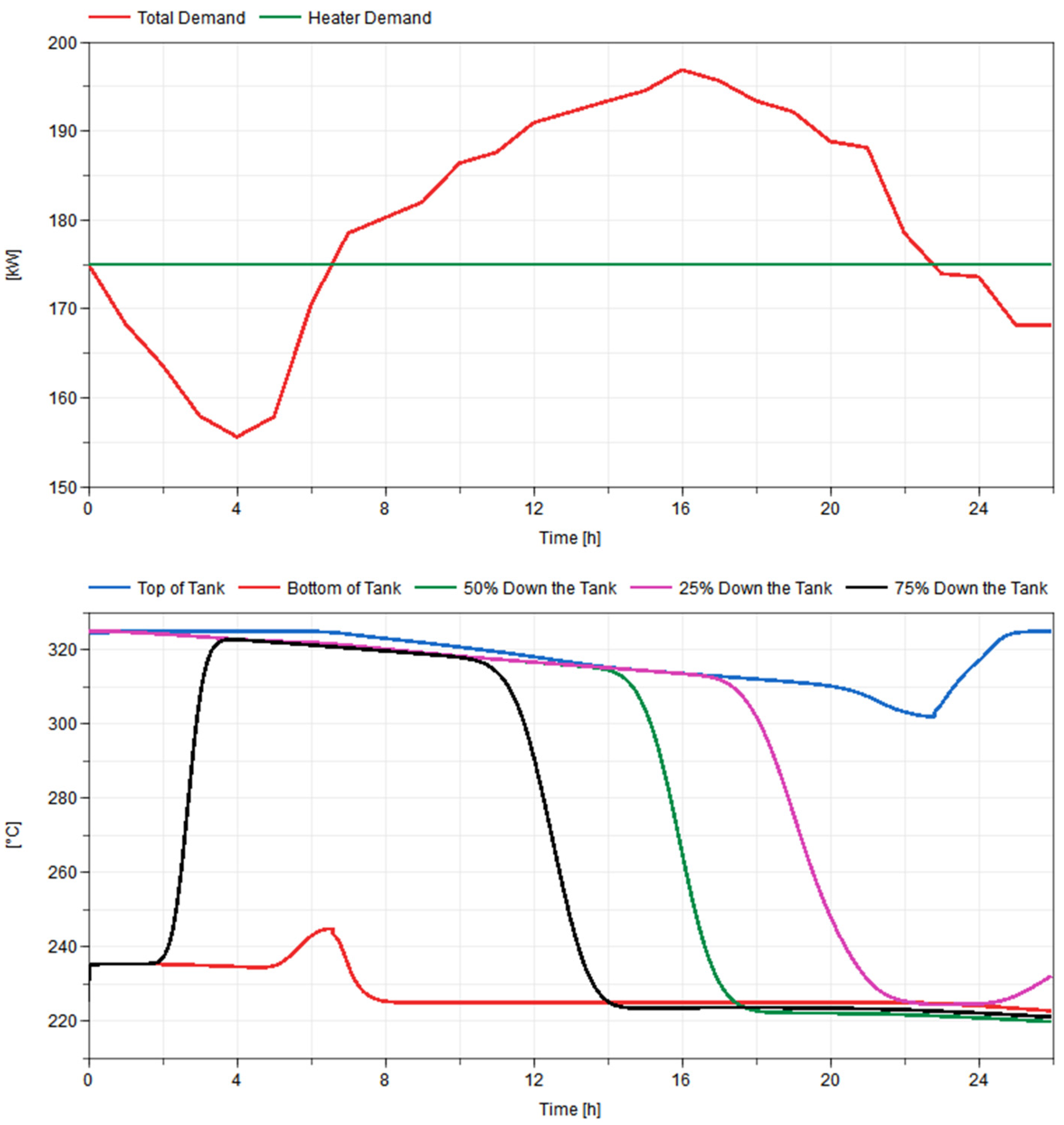
4.2. Summer-Day Test

The previously described simulation demonstrates the system’s capability to operate throughout all foreseeable operating modes. One advantage of TEDS is that it can be used to size system components relative to regional grid buildout. To demonstrate this ability, TEDS was subjected to a load typical of a hot summer day [16] in an area with mixed commercial and residential electricity needs (Figure 14). The system was sized to represent a nuclear generator coupled to a thermal-storage unit with 12.5% peaking capacity in a constrained grid scenario. So, at peak demand, the thermal-storage unit could be utilized as a peaking unit to meet that demand. The mean net demand could be met solely by the nuclear generator, and, in times of low net electricity demand (Net demand = Total Demand − Renewable Energy), excess capacity could be stored in the thermal-storage tank. The system parameters were identical to those found in Table 5. The full twenty-five-hour simulation took 429 s.

Initially, the thermal storage tank was assumed to be 66% charged. The first hour of the simulation served to stabilize the system from a numerical perspective, and charging-side temperatures were higher than 225 °C because of initialization conditions on the tank walls. hour 1 corresponded to midnight. Starting from “time zero,” the demand was lower than the potential Chromalox heater output, so the excess capacity was sent to the thermocline tank for storage. This process continued for the next five-and-a-half hours, with a maximum charging rate of 20 kW occurring at hour 4 (3 a.m.). Then, at the six-and-a-half-hour mark (5:30 a.m.), as people got ready to start their days, the temperature began to rise, air conditioning units turned on, the total demand reached the maximum output of the Chromalox heater, and the charging ceased. From hour 6 to hour 22 (9:00 p.m.), the demand exceeded the heater output, triggering the discharge operation. During this operation, hot fluid from the thermocline tank was sent to the chiller to simulate the amount of heat required to boil steam and produce energy for the community. Throughout the discharge cycle, cold fluid was pumped into the bottom of the chiller while hot fluid was pumped out.

During the simulation, heat loss to ambient surroundings dramatically decreased the temperature throughout the thermocline tank, as shown in Figure 14. This was exacerbated by flow from colder regions of the tank mixing with hotter regions during the charge/discharge cycles. This heat loss, though minor over the course of a single hour, becomes more pronounced when the heat is stored for long periods of time. The initial discharge exit temperature was ~325 °C; by hour 21, ambient heat loss and internal mixing in the tank had reduced this to ~310 °C. Such degradation leads to efficiency losses in the overall process, and, at a certain point, the outlet temperature falls below a “useful” threshold. Moving forward, it is important that this phenomenon be incorporated into the system control strategy for IES that intend to utilize packed-bed thermocline systems.

Heater power throughout the run was kept at 175 kW, except for slight fluctuations occurring as the system transitioned from mode to mode, as shown in Figure 15. The Chromalox heater’s exit temperature was maintained at 325 °C throughout the simulation, and the ethylene glycol flow rate never decreased to the point at which boiling potentially occurs, as the heat exchanger always maintained an inlet temperature higher than the exit temperature setpoint of 225 °C.

Throughout the run, the heater demand never dropped to zero and triggered GBV-006 to close. Instead, GBV-006 modulated throughout the run to meet heater demand without any major over- or under-shoot in mass flow. Thermal-storage demand, however, operates on smaller signals and via an interlocking valve on both the charge and discharge lines. Thermal-storage demand is negative by convention if charging is desired, and positive if discharge is desired. During charging, GBV-201 modulated in accordance with the desired demand, and FM-201 matched the charging demand with the charging flowrate, with little to no overshoot apart from hour 23, in which a massive overshoot occurred as the valve first began to open, illustrated in Figure 16. This is attributable to three things. First, the long period of zero demand on the valve meant there was a large windup of integral term error in the signal. Second, the charging and discharge lines operated on interlocks to ensure that both lines were never open simultaneously. Third, valve modulations when first opening had a much larger effect on mass flow fluctuations than when opening in the middle band of valve position. Similarly, during discharge, GBV-202 modulated in accordance with the desired demand, and FM-202 matched the discharge demand with little to no overshoot apart from a little past Hour 6, when a massive overshoot occurred as the valve first began to open. This overshoot was quickly subdued, and GBV‑202 was able to meet the discharge demand.

5. Conclusions

Model development has led to the creation of a dynamic systems-level model of the experimental TEDS facility in the Modelica language, capable of operating under all potential modes set forth by the design team. Development included the creation of property modules for therminol-66, alumina, FOAMGLAS^® ONE, and ethylene glycol (DowTherm SR-1) all of which have been incorporated into the TRANSFORM library at ORNL. Control algorithms were developed to be consistent with exposed variables within TEDS to enable seamless integration of the control algorithms proposed in this report. The model includes the primary components of the TEDS experimental unit, including a 200 kW Chromalox heater designed to simulate a light-water reactor heat source, a single-tank packed-bed thermal-energy storage system filled with 0.125 in. alumina (Al₂O₃), an ethylene-glycol-to-therminol-66 heat exchanger, system piping, five control valves, and all associated temperature, pressure, and mass flow sensors. The model does not include nitrogen-fill gas tanks or associated overfill tanks, as these are not part of standard system control.

The model was used during the pre-construction phase of the experimental effort in order to inform the experimental design (e.g., insulation requirements, bypass line placement, expected performance of components) and test innovative control schemes prior to initial operation. Through the simulation, it was determined that the thermocline tanks required a 6 in. layer of FOAMGLAS^® ONE insulation to help minimize heat loss while still fitting within the physical footprint of the experiment. Additionally, it was determined that a bypass line on the therminol-66 side of the heat exchanger, or a minimum ethylene glycol mass flow rate, is required to ensure that no boiling of the ethylene glycol can occur during Mode 4 or Mode 2 operations. This requirement is resulting in the inclusion of a not-previously-envisioned bypass line on the oil side of the oil-glycol heat exchanger.

Two simulation sets were run. The first was a 5 h shakedown test of the system, putting it through all five potential operating modes and showcasing the ability of the valving, control sensors, and component controllers to meet system demands. During shakedown testing, it was noted that a minimum mass flow rate of 0.05 kg/s on the ethylene glycol chiller is required to ensure that bulk boiling of the glycol does not occur. This requirement led to a ~15 kW increase in heater power to ensure that exit temperatures were maintained at 325 °C. In the future, a bypass line will be installed on the therminol-66 side of the heat exchanger to mitigate this issue.

The second case imposed a typical-summer-day demand from a region with mixed commercial and residential electrical needs on the system—a case in which the generator alone could not meet peak demand, but instead required the thermal storage unit to act as a peaking unit. Over the course of the “day”, the valving and sensors were able to meet the demand, as expected. However, a large amount of thermal degradation occurred due to external heat loss. Over the course of the 15 h discharge cycle, heat loss accounted for a drop of approximately 15 °C in outlet temperature. Such heat loss decreases the overall system efficiency and may lead to additional design changes in the future, such as the possible inclusion of a topping heater.

Through the commencement of this work, a systems-level model of TEDS—along with associated control systems, sensors, piping diameters, and component capabilities—was created. This model was utilized in the pre-experimental phase to inform system design, insulation thicknesses, bypass line placement, and potential control schemes for operating the system effectively and safely. TEDS is currently being installed and will begin operation in December 2020. Operational data will be used to validate, refine, and tune the TEDS model. This refined model will then be used as a starting point for designing experimental systems intended for integration with TEDS within the laboratory setting. Additionally, through the creation of a TEDS model and a corresponding experimental facility that will initially be used to validate the simulation model, research organizations and industry will be able to demonstrate their technologies both digitally and experimentally. In the initial stages, researchers can leverage the existing TEDS Modelica model to test any number of new and unique control strategies, coupling mechanisms, ancillary processes, system sizing, and system response to various externalities, such as market conditions. Researchers and industry partners then will be able to bring their technologies into the lab to verify their selected computational permutation and obtain data for validation, verification, and licensing purposes.