Speed Fluctuation Suppression for the Inverter Compressor Based on the Adaptive Revised Repetitive Controller

Abstract

Repetitive operation is extensively present in the inverter compressor refrigeration field. Research illustrates that an approximate periodic load disturbance deteriorates its self-sensing and efficiency in a low frequency range. According to an internal model theorem, a repetitive controller can realize periodic signal tracking or suppression; however, ideal repetitive control (IRC) can not be directly employed in practical application owing to its excessive sensitivity to period-time uncertainties or aperiodic component, etc. In addition, the ratio between period delay to sampling time can not always maintain an integer which causes the resonant frequencies to deviate from the interested. Even if the ratio is a fixed integer, the auxiliary function for stabilization in a conventional repetitive controller can result in the steady state tracking error. In this paper, a revised repetitive controller with a novel Savitzky–Golay (S–G) filter is proposed, the S–G filter cascaded with a traditional delay element can approximate the delay element with any ratio. Aiming at a different operating condition, a second order generalized integrator (SOGI) based observer is employed to extract disturbance fundamental component, and Steiglitz–McBride based adaptive notch filter (SM-ANF) is adopted for frequency estimation. The proposed scheme varies the S–G filter according to variable fundamental frequency and maintains its resonant frequencies corresponding with the fundamental and harmonic disturbance. In the end, simulations and experiments are implemented and results illustrate that speed fluctuation can be effectively suppressed by the proposed method.

1. Introduction

Owing to the characteristics of a simple structure, high power density, wide speed range and easy implementation, induction motor (IM) has been extensively replaced by a permanent magnetic synchronous motor (PMSM) in the inverter compressor refrigeration field. Generally, the refrigeration system mainly consists of an inverter compressor (PMSM), condenser, throttling device, and evaporator, where an inverter compressor can be divided into several types: rotating (single and double), scroll and centrifugal, etc., a single rotor inverter compressor has a large market share in the refrigeration field because of its characteristics in energy efficiency ratio (EER) and cost performance ratio. Inverter compressor, being the central part of refrigeration system, conducts refrigerant suction, compressor and exhaust periodically, then the pressure gap between left and right volume can be considered as an external disturbance for an inverter compressor, which can ruin its normal operation characteristics, such as speed ripple, self-sensing control, and vibration, etc. As a result, how to realize stable operation with high EER, in other words, how to suppress torque ripple and corresponding speed fluctuation, is a critical issue in the refrigeration field.

In order to suppress speed fluctuation in the inverter compressor driving system, extensive research has been conducted and some effective methods have been proposed. At present, the general method in engineering application is sinusoidal torque compensation, which neglects harmonic components of load disturbance, then torque ripple and corresponding speed fluctuation is still apparent. Zhang in the Midea group adopted fast Fourier transformation (FFT) to extract speed fluctuation components and deduced current compensation to suppress speed fluctuation in low frequency range [1]; however, disturbance harmonic components are neglected and fluctuation suppression performance is unsatisfactory. Huang in the Gree group proposed a method that can automatically achieve torque compensation [2], which is essentially a general disturbance observer (DOB) suitable to constant or slow varying disturbance, but disturbance harmonic components can not be effectively rejected owing to its small sensitivity gain; consequently, Huang’s method is not suitable for periodic disturbance compensation. From the analyses mentioned above, it can be observed that both methods have some limitations which can be inappropriate for periodic disturbance suppression; then, the corresponding speed fluctuation ratio is still obvious in a low frequency range.

In general, disturbance/uncertainty estimation and attenuation (DUEA) [3,4] are widely employed in the PMSM driving system. Compared to traditional closed-loop feedback control, disturbance compensation can directly and effectively realize disturbance rejection; however, disturbance can not be measured or be difficult to measure by sensor device. To solve this issue, two methods were proposed: one is disturbance observer (DOB) [5]; the other is active disturbance rejection control (ADRC) [6]. Iterative learning control (ILC) is actually an error correction algorithm and memory storing the previous controller output and error information, which can be employed to suppress periodic torque ripple by operating repetitively over a fixed time interval. Model predictive control (MPC) with ILC was proposed in literature [7] to enhance speed dynamics; moreover, the forgetting factor was introduced to ensure closed loop robustness against noise, initialization error, and fluctuation of system dynamics; however, torque ripple can be ensured within a certain bound. Modified ILC in the frequency domain by means of Fourier series expansion was employed to further reduce torque ripple in literature [8], which takes an averaging operation on noise and can remove the majority of noise and aperiodic components; the deficiency is that external disturbance is not taken into consideration in the two methods above. The nonlinear control complicated design procedure and a lot of parameter adjustment make ADRC difficult to implement in practical application; linear ADRC (LADRC) was proposed in literature [9] to enhance speed robustness; moreover, a load disturbance observer (it is essentially a Luenberger observer) cascaded with linear ESO (LESO) are employed to compensate disturbance, but it is available to a constant or slow varying disturbance. Sliding mode control (SMC), being a well-known nonlinear controller, can provide an effective and systematic approach to maintain consistent stability with good robustness. In the design of an SMC, a suitable switch gain should be selected, although a large switch gain can ensure that anti-disturbance performance, discontinuous control signal, and serious switching chattering will exist. Consequently, SMC cascaded with DOB are widely employed to achieve fast convergence ratio, high tracking accuracy, and robustness against load disturbance. A second-order non-singular terminal sliding mode observer (SONST-SMO) was proposed in literature [10], compared to general SMO, which takes advantage of both high-order sliding mode and non-singular terminal sliding mode to achieve fast convergence ratio and reduce switching chattering. Similarly, an ESO based improved continuous fast terminal sliding mode control (ICFT-SMC) was proposed in literature [11] for speed regulation, where a high switching gain is unnecessary compared to CFTSMC. Adaptive sliding mode control (ASMC) with a sliding mode disturbance observer (SM-DOB) was proposed in literature [12], where ASMC was introduced to improve current loop dynamics and robustness to parameter deviation, SM-DOB was adopted to compensate external disturbance and reduce ASMC switch gain. Although the above three methods can achieve fast dynamics and robustness, a complicated design procedure and a lot of parameter adjusting make it difficult for practical application.

RC, originally put forward by Nakano, can realize better suppression/tracking performance by constructing an appropriate internal model [13,14,15,16,17]; its simple structure and easy implementation characteristics make it extensively employed in power electronic fields, including but not limited to: voltage source inverter (VSI) [18,19], and PMSM driving [20,21,22], etc. RC cascaded with low pass filter (LPF) was adopted in literature [18] to improve robustness; however, amplitude attenuation and phase delay in high frequency range are obvious, which cause disturbance suppression performance to deteriorate. Aiming at the phase delay problem brought about by RC, a phase lead item was introduced in literature [23] to satisfy stability requirements in the closed loop system. Aiming at specific frequency harmonic disturbance, phase compensation can be employed to broaden loop bandwidth, and an appropriate gain of RC can be determined to satisfy stability requirements [24]. However, this method is sensitive to period-time variation or uncertainties, and it is unsuitable to suppress speed fluctuation for an inverter compressor driving in a variable operating condition.

In practical application, a fraction (the ratio between period-time to sampling time) can be generally substituted by the nearest integer in RC discretization; then, the deviation between approximated and real disturbance internal model can result in poor disturbance suppression performance. In particular, the aperiodic components may lead to system instability. Consequently, the correction and optimization to disturbance internal model is one of the research hotspots in RC design. RC with fictitious sampling was proposed in [25], and the ratio of fictitious sampling period to grid period-time can be maintained as an integer; however, the fictitious sampling period was obtained from a practical sampling points deviation; then, disturbance frequencies will shift away the interested. A low pass filter cascaded with delay element was introduced to enhance RC’s robustness [26], where the actual delay element slightly less than the reference can be acquired by strict derivation. In addition, an excellent dynamic response can be confirmed (tracking error can be small after approximately five cycles). Aiming at voltage harmonics under a variable frequency grid, a variable delay element was employed to obtain a more accurate internal model [27], although main harmonics can be perfectly suppressed, and phase delay brings the rest of the resonant frequencies deviating from the interested. To solve this problem, a revised FIR filter was adopted in [28]; in addition, period delay in a continuous domain can be well approximated by an integral delay element cascaded with a revised FIR filter in a discrete domain. Aiming at $6k\pm 1$-th harmonics ($k\in \mathbb{Z}$) in a three-phase grid-connected inverter, the delay element in a continuous domain was approximated by an integral delay element cascaded with linear interpolation (it is generally a one order FIR filter) in a discrete domain [29]. However, a normalized cut-off frequency was required in two previous works and is inappropriate for high frequency disturbance, such as model uncertainties, etc. Using a Lagrange interpolation polynomial to approximate period delay in continuous domain was proposed in [19], and, compared to general RC, it can suppress any frequency disturbance theoretically because of amplitude fluctuation and phase lag brought about by LPF; disturbance suppression performance is unsatisfactory in a high frequency range. Moreover, high accurate approximation can result in a computational burden, and it is necessary to make a trade-off between disturbance suppression performance and dynamic response.

In order to resolve the issue mentioned above, the S–G filter cascaded with RC is proposed in this paper, which also has the following characteristics:

• It is convenient to activate or suspend RRC without affecting system normal operation.
• S–G filter implementation is simple and only consumes a small amount of multiplications and additions, which maintains the resonant frequencies corresponding with fundamental and harmonic disturbance.

Moreover, deterioration of suppression performance owing to different operating condition or period-time uncertainties is also a critical issue; consequently, fundamental frequency estimation is adopted to achieve adaptive characteristic [30]. Because adaptive notch filter (ANF) is extensively employed in signal processing [31], such as signal separation and enhancement, etc., the Steiglitz–McBride method is well known for its simple implementation, fast convergence ratio, and unbiased online estimation; therefore, ANF based on Steiglitz–McBride (SM-ANF) [32] is employed to estimate fundamental wave frequency.

The paper is organized as follows: the overall structure of inverter compressor control system is described in Section 2; in Section 3, the Savitzky–Golay (S–G) filter and the revised repetitive controller are introduced; in addition, the design method and implementation are presented; in Section 4, a disturbance observer based on a second order generalized integrator (SOGI) is proposed to extract a disturbance fundamental wave, and fundamental frequency is estimated by SM-ANF; in Section 5, simulation and experimental results are presented, which demonstrate validity and effectiveness of the proposed scheme.

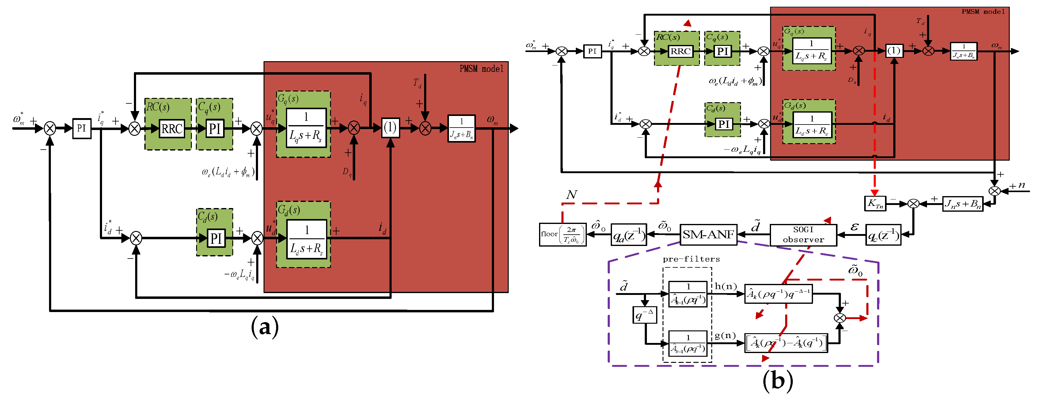
2. System Modeling and Analysis

The structural diagram of inverter compressor (single rotor) is presented in Figure 1a, which is mainly composed of motor (PMSM), cylinder (pressure boosting), housing (supporting and sealing) and reservoir (filtering), etc. The refrigeration loop of air-conditioner is presented in Figure 1c; firstly, low-temperature and low-pressure gaseous refrigerant becomes high-temperature and high-pressure gaseous refrigerant by continuous compression; secondly, high-temperature and high-pressure gaseous refrigerant is condensed to high-temperature and high-pressure liquid refrigerant by water or air in the exterior; thirdly, high-temperature and high-pressure liquid refrigerant becomes low-temperature and low-pressure liquid refrigerant through capillary (expansion valve) regulating; moreover, the refrigerant amount is dominated by thermal load and refrigeration velocity, etc.; fourthly, low-temperature and low-pressure liquid refrigerant is evaporated to low-temperature and low-pressure gaseous refrigerant and the interior temperature drops. Because the cylinder is divided into left and right volume by eccentric piston and slider, left and right volume driven by motor conduct refrigeration suction, compression and exhaust alternatively, which results in load torque presenting approximately periodic characteristics [2]. In addition, different operating conditions (pressure gap and temperature gap, etc.) can result in load torque difference. Figure 2 [2] illustrates load torque under different operating conditions, and it can be observed that load disturbance presents approximately sinusoidal with respect to a rotor mechanical angle; meanwhile, magnitude and phase have significant differences.

Suppose that: 1. rotor core without saturation; 2. without taking into consideration eddy current loss; 3. flux brought about by phase current and permanent magnet with sinusoidal distribution. Under synchronous rotating $d-q$ reference frame, the motion equation of inverter compressor can be expressed as follows:

$$\left\{\begin{array}{cc}\hfill \frac{d{\omega }_m}{dt}& =\frac{1}{J}(T_e-T_d)-\frac{B}{J}{\omega }_m\hfill \\ \hfill T_e& =\frac{3}{2}{n}_p\left[{\varphi }_m{i}_q+(L_d-L_q)i_d{i}_q\right]\approx \frac{3}{2}{n}_p{\varphi }_m{i}_q\approx K_T{i}_q\hfill \\ \hfill K_T& =\frac{3}{2}{n}_p{\varphi }_m\hfill \\ \hfill \frac{d{i}_d}{dt}& =\frac{1}{L_d}\left(u_d-R_s{i}_d+n_p{\omega }_m{L}_q{i}_q\right)\hfill \\ \hfill \frac{d{i}_q}{dt}& =\frac{1}{L_q}\left(u_q-R_s{i}_q-n_p{\omega }_m(L_d{i}_d+{\varphi }_m)\right)\hfill \end{array}\right.$$

(1)

where $n_p$, ${\varphi }_m$, $R_s$, $K_T$, ${\omega }_m$, J, and B represent pole pairs, rotor permanent magnetic flux, stator winding resistance, equivalent electro-magnetic constant, mechanical angular speed, moment of inertia and viscosity coefficient, respectively; $i_d$ and $i_q$ represent $d-q$ axis current, respectively; $L_d$ and $L_q$ represent $d-q$ axis inductance, respectively; $T_d$ represents lumped disturbance, which mainly consists of harmonic disturbance, unmodeled dynamic disturbance, and load disturbance, etc.

It can be known that an inverter dead-zone nonlinear voltage drop mainly produces $6k\pm 1$-th ($k\in \mathbb{Z}$) voltage harmonics under $\alpha -\beta$ reference frame [21], that is to say, $6k$-th harmonics under $d-q$ reference frame after Park transformation; then, corresponding torque ripple is introduced. It is noteworthy that current harmonics are slightly weaker in a high frequency range; in addition, smaller energy makes it difficult to cause speed fluctuation. Consequently, speed fluctuation brought about by load disturbance is the main factor in this paper. In order to simplify control system design, the following assumptions are necessary:

• Assumption 1: Load disturbance has identical periodicity and repetitiveness under almost the same operating condition.
• Assumption 2: The control objective aims to suppress speed fluctuation repetitively under almost the same operating condition.
• Assumption 3: Measurement noise mainly exists in the high frequency range, and the general low pass filter can filter off effectively.

The equivalent control block diagram of inverter compressor driving system is presented in Figure 3a, where electrical angular speed between stator flux and rotor permanent magnetic flux is regulated for torque optimized efficiency, $M_d$ and $M_q$ represent $d-q$ axis VSI nonlinear voltage drop, respectively, $G_{pi}\left(s\right)$ and $G_p\left(s\right)$ represent PI controller and load admittance, respectively, $K_p^{d\left(q\right)}$ and $K_i^{d\left(q\right)}$ represent $d-q$ axis proportional and integral coefficient, respectively, which can be determined by an I type system parameter tuning method. Although the PI controller can track a reference with a negligible steady state error and be robust against DC or low frequency disturbance, periodic disturbance can not be effectively suppressed because the sensitivity gain at disturbance related frequencies is small. The control block diagram of inverter compressor with general DOB is presented in Figure 3b. DOB, being a two degree of freedom controller based on an observer structure, can achieve high pass sensitivity and low pass complementary sensitivity because sensitivity corresponds to disturbance suppression performance and complementary sensitivity corresponds to noise sensitivity and robust stability [33,34]. For constant or slow varying disturbance, the trade-off between sensitivity and complementary sensitivity can be achieved through an appropriate cut-off frequency; disturbance can be effectively compensated and corresponding speed fluctuation can be asymptotically rejected; however, owing to the small sensitivity gain at fundamental and harmonic frequencies, periodic disturbance can not be effectively compensated by general DOB and corresponding speed fluctuation suppression performance is unsatisfactory.

3. Revised Repetitive Controller Analysis and Design

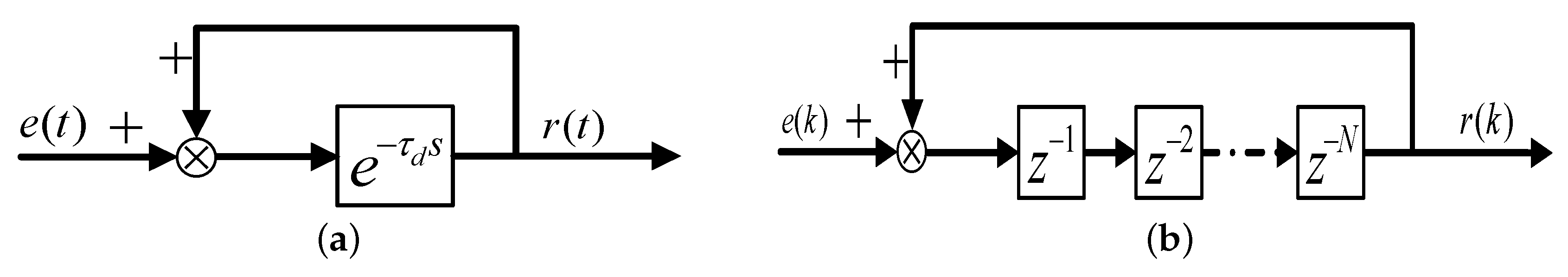
3.1. Ideal Repetitive Controller

The structural diagram of ideal repetitive controller (IRC) is presented in Figure 4a, where $G_c\left(z^{-1}\right)$ represents an existing controller ($\mathrm{PID}$ or ${\mathrm{H}}_{\infty }$ controller) based on loop shaping method to achieve some characteristics (servo or robust characteristic), $G_p\left(z^{-1}\right)$ represents control plant, $q\left(e^{-j\omega T_s}\right)={\omega }_c/(j\omega +{\omega }_c)$ represents low pass filter with cut-off frequency ${\omega }_c$ ($T_s$ represents sampling period), d represents external disturbance, $G_{RC}\left(z^{-1}\right)$ in the red dashed line represents internal model of period disturbance. It can be observed that sensitivity function $S_{IRC}\left(z^{-1}\right)$ is equal to zero at fundamental and harmonic frequencies illustrating that output y can track reference r with negligible error in the steady state, where $S_0\left(z^{-1}\right)$ represents the sensitivity function of original system without RC; in other words, periodic disturbance can be effectively rejected:

$$\left\{\begin{array}{cc}\hfill S_{IRC}\left(z^{-1}\right)& =S_0\left(z^{-1}\right)\times \frac{1-z^{-N}}{1-(1-H\left(z^{-1}\right))z^{-N}}\hfill \\ \hfill S_0\left(z^{-1}\right)& =\frac{1}{1+G_c\left(z^{-1}\right)G_p\left(z^{-1}\right)}\hfill \end{array}\right.$$

(2)

where $H\left(z^{-1}\right)=G_p\left(z^{-1}\right)/(1+G_c\left(z^{-1}\right)G_p\left(z^{-1}\right))$. Supposing that the system is stable, then the following condition should hold:

$$\begin{array}{c}\hfill \left|1-H\left(z^{-1}\right)\right|<1\end{array}$$

(3)

As a matter of fact, IRC can not be directly employed in practical application. Firstly, IRC is over sensitive to uncertainties, although yielding perfect disturbance suppression characteristics, the robustness of closed loop is generally unsatisfactory; secondly, IRC is influenced by aperiodic disturbance, such as non-periodic performance: bringing the sensitivity gain down to zero at fundamental frequency and its multiples is paid for by an increased sensitivity at intermediate frequencies [16], although auxiliary function $q\left(z^{-1}\right)$ in Figure 4a can improve robustness to uncertainties, amplitude attenuation, and phase delay become apparent with frequency increasing, which can jeopardize disturbance suppression performance, closed loop stability may be seriously destroyed; thirdly, more accurate measurement of period-time is required to implement IRC, which may be affected by estimation accuracy, measurement noise, etc.; in the end, only the ratio between period-time to sampling time being an integer can RC be implemented, generally, adopting the nearest value to substitute the real can bring resonant frequencies deviating from the interested. Therefore, how to construct RC with adaptiveness and robustness is a critical issue to be resolved.

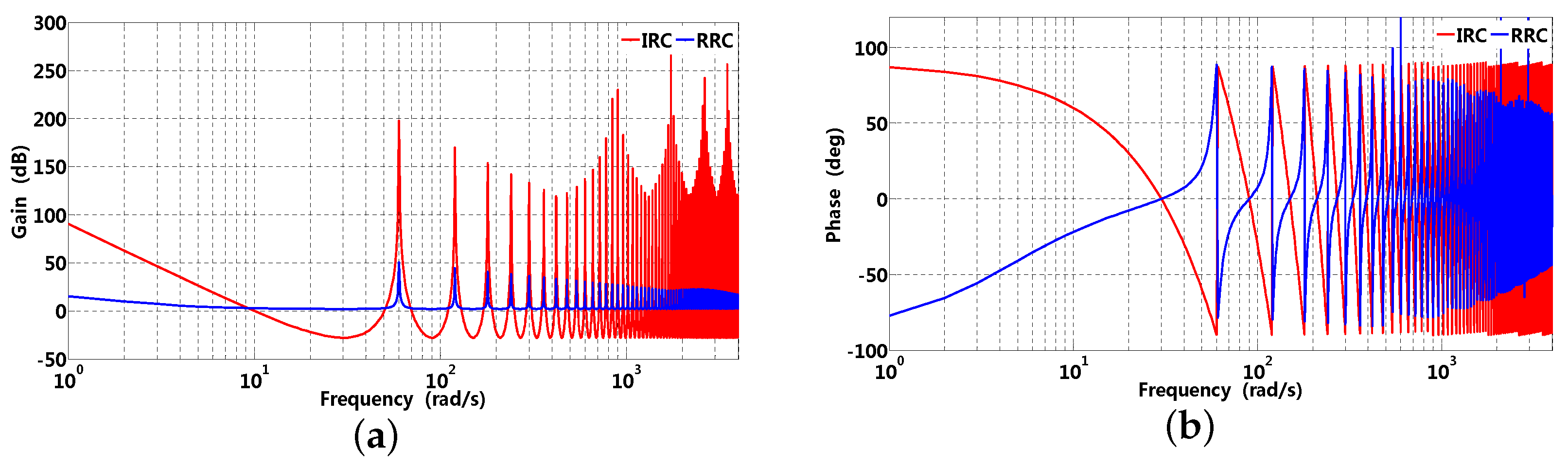
3.2. Revised Repetitive Controller

The block diagram of disturbance internal model is presented in Figure 5, where the disturbance internal model in the discrete domain consists of an N delay unit satisfying the principle first in first out (FIFO). However, only when the ratio is an integer can RC be implemented. In addition, it is generally to adopt auxiliary function $q\left(z^{-1}\right)$ to enhance robustness. When $q\left(z^{-1}\right)$ is selected as a constant slightly smaller than the unit, internal model deviation brings resonant frequencies deviating from the interested; in addition, a disturbance suppression error can exist in the steady state and complementary sensitivity characteristic is poor; when $q\left(z^{-1}\right)$ is selected as a general LPF, although it has a unit gain in a low frequency range, a complementary sensitivity characteristic in a high frequency range is unsatisfactory, even if delay element is integral.

Supposing that function $q\left(z^{-1}\right)z^{-N}$ can approximate delay element $e^{-{\tau }_{d}s}$, better disturbance suppression performance and robustness to frequency uncertainties, measurement noise, and aperiodic component can be confirmed. Defining $N_{int}$ as an integer slightly smaller than $N={\tau }_d/T_s$, then the phase of $e^{-(N-N_{int})T_{s}s}$ can be expressed as follows:

$$\begin{array}{c}\hfill {\left.\angle e^{-(N-N_{int})T_{s}s}\right|}_{s=j\omega }=\angle e^{-j\omega (N-N_{int})T_s}=-(N-N_{int})\omega T_s\end{array}$$

(4)

Equation (4) illustrates that the phase characteristic of $q\left(z^{-1}\right)$ should be linear. S–G filter, originally proposed by Savitzky and Golary, has low-pass and linear-phase characteristics, which can filter off high frequency noise by polynomial interpolation. In addition, larger cut-off frequency can be acquired at the sacrifice of noise reduction ratio (NRR) compared to FIR. Consequently, the S–G filter can satisfy the phase requirement and its transfer function can be expressed as:

$$\begin{array}{c}\hfill q\left(z^{-1}\right)=\sum _{k=0}^{2p}{a}_k{z}^{-k}\end{array}$$

(5)

It can be known that the phase characteristic of traditional S–G filter is determined by order p and can only be $-0.5\omega T_s$, $-\omega T_s$, $-1.5\omega T_s$, ⋯, [35]. Here, a novel design methodology of S–G filter is proposed as follows, and its coefficients satisfy

$$\begin{array}{c}\hfill a_{2p-k}=\frac{D-k}{(2p-k)-D}{a}_k\end{array}$$

(6)

where the coefficients $a_k$ ($0⩽k⩽p$) can be calculated according to quadratic polynomial interpolation, D is selected as $p-1<D⩽p$. S–G filter with phase characteristic in Equation (4) can be satisfied based on Equations (5) and (6), and the design procedure is presented as follows.

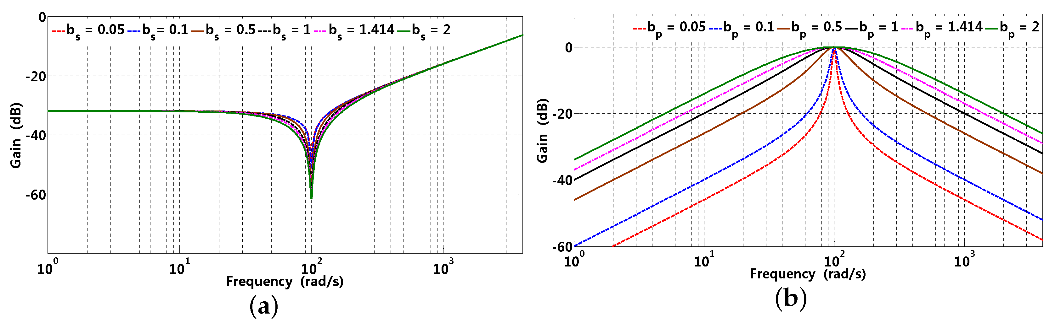
3.2.1. Coefficients of the S–G Filter

Defining $p$-order interpolation polynomial

$$\begin{array}{c}\hfill q=a_0+a_{1}i+a_2{i}^2+\cdots +a_p{i}^p=\sum _{k=0}^p{a}_k{i}^k,p\le 2M\end{array}$$

(7)

to smooth $x\left(i\right)$, $i=-M,\cdots ,0,\cdots ,M$, in addition, optimal criterion function based on sum of square error can be written as:

$$\begin{array}{c}\hfill min\left(E\right)=min\left(\sum _{i=-M}^M{\left[q-x\left(i\right)\right]}^2\right)=min\left(\sum _{i=-M}^M{\left[\sum _{k=0}^p{a}_k{i}^k-x\left(i\right)\right]}^2\right)\end{array}$$

(8)

Taking partial derivative about Equation (8)

$$\begin{array}{c}\hfill \frac{\partial E}{\partial a_r}=\frac{\partial }{\partial a_r}\left[\sum _{i=-M}^M{\left(\sum _{k=0}^p{a}_k{i}^k-x\left(i\right)\right)}^2\right]=2\sum _{i=-M}^M\left[\sum _{k=0}^p{a}_k{i}^k-x\left(i\right)\right]i^r=0,r=0,1,\cdots ,p\end{array}$$

(9)

Make simplifications and the following can be derived:

$$\begin{array}{c}\hfill \sum _{k=0}^p{a}_k\sum _{i=-M}^M{i}^{k+r}=\sum _{i=-M}^{M}x\left(i\right)i^r\end{array}$$

(10)

Defining:

$$\begin{array}{c}\hfill Q_r=\sum _{i=-M}^{M}x\left(i\right)i^r,S_{k+r}=\sum _{i=-M}^M{i}^{k+r}\end{array}$$

(11)

Then, Equation (10) yields:

$$\begin{array}{c}\hfill Q_r=\sum _{k=0}^p{a}_k{S}_{k+r}\end{array}$$

(12)

For given M, polynomial order p and interpolation data $x\left(i\right)$, coefficient $a_k$ can be calculated with Equation (12) and S–G filter can be determined. As a matter of fact, not all coefficients are necessary, it is evident

$$\left\{\begin{array}{cc}\hfill {\left.q\right|}_{i=0}& =a_0\hfill \\ \hfill {\left.\frac{dq}{di}\right|}_{i=0}& =a_1\hfill \\ \hfill & ⋮\hfill \\ \hfill {\left.\frac{d^{p}q}{d{i}^p}\right|}_{i=0}& =p!a_p\hfill \end{array}\right.$$

(13)

that $a_0=q$ at central point $i=0$; furthermore, coefficients $a_1$, $a_2$, ⋯ $a_p$ are proportional to the $1$-st, $2$-nd, ⋯ $p$-th derivative at central point, respectively. As a result, if $a_0$ can be calculated based on Equation (10), it can be confirmed that polynomial $f_i$ is the optimum fitting at central point $x\left(0\right)$, in addition, S–G filter only needs a small amount of additions and multiplications for coefficients calculation. It is noteworthy that the computational complexity can further reduce if $k+r$ is odd in Equation (12).

3.2.2. Phase Characteristics

The phase of Equation (5) can be derived as:

$$\begin{array}{cc}\hfill \angle q\left(z^{-1}\right)& =\angle q\left(e^{-j\omega T_s}\right)=\angle \left\{\sum _{k=0}^{2p}{a}_k\left[cos\left(k\omega T_s\right)-jsin\left(k\omega T_s\right)\right]\right\}\hfill \\ \hfill & =-{tan}^{-1}\frac{{\displaystyle \sum _{k=0}^{2p}}{a}_{k}sin\left(k\omega T_s\right)}{{\displaystyle \sum _{k=0}^{2p}}{a}_{k}cos\left(k\omega T_s\right)}\hfill \end{array}$$

(14)

Supposing that the S–G filter phase characteristic can satisfy the requirements in Equation (4), making $D=N_{int}-N$, the following can be obtained:

$$\begin{array}{c}\hfill -\frac{{\displaystyle \sum _{k=0}^{2p}}{a}_{k}sin\left(k\omega T_s\right)}{{\displaystyle \sum _{k=0}^{2p}}{a}_{k}cos\left(k\omega T_s\right)}=tan(-D\omega T_s)=-\frac{sin\left(D\omega T_s\right)}{cos\left(D\omega T_s\right)}\Rightarrow \sum _{k=0}^{2p}{a}_{k}sin\left[(D-k)\omega T_s\right]=0\end{array}$$

(15)

In the low frequency range, fundamental and main harmonic frequencies are smaller than the sampling frequency, then Equation (15) can be simplified as:

$$\begin{array}{c}\hfill sin\left[(D-k)\omega T_s\right]=(D-k)\times sin\left(\omega T_s\right).\end{array}$$

(16)

There is always be a middle term $k=p$ in Equation (15); however, it is small and can be neglected; therefore, Equation (15) is proven to be true, which signifies that the S–G filter of Equation (5) and (6) can approximate delay element $e^{-{\tau }_{d}s}$ in the low frequency range; then, sensitivity and robustness of RRC can be guaranteed.

3.2.3. Selection of D

It is noteworthy that, when D is selected as p, coefficients of the S–G filter in Equation (6) can be simplified as $a_{2p-k}=a_k$ ($0⩽k<p$), which is identical with traditional S–G filter. Generally, D is selected around p; in addition, $N_{int}$ should be slightly smaller than ratio N [17], which requires that D should be slightly larger than zero, and the order of S–G filter is not too high; then, D is selected as $p-1<D⩽p$ in this paper.

In the end, the design procedure of S–G filter is summarized as follows. First, cut-off frequency, sensitivity gain, and current sampling noise should be taken into consideration when selecting the order of S–G filter; second, D is selected between $p-1$ and p; moreover, the coefficients $a_k$ ($0⩽k⩽p$) are calculated according to Equation (12), and coefficients of $a_k$ ($p+1⩽k⩽2p$) are obtained with Equation (6).

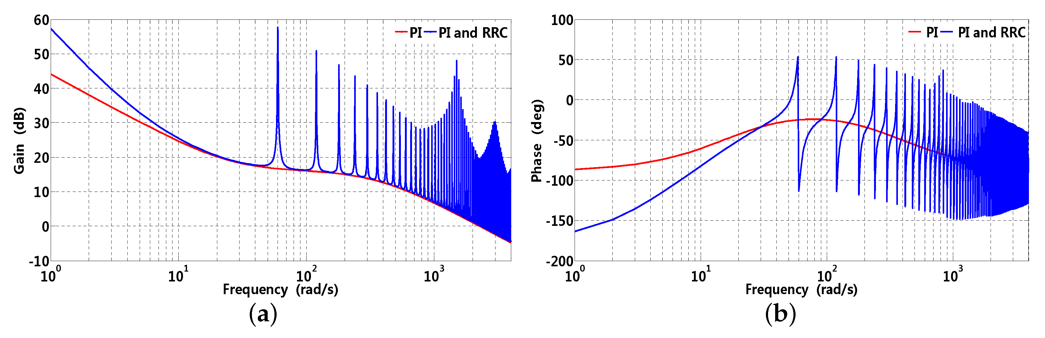
3.3. RRC Implementation

The order of S–G filter is determined by cut-off frequency, sensitivity gain, and current sampling noise, etc. On one hand, if current sampling is noisy, a larger p can improve NRR; on the other hand, larger NRR can result in cut-off frequency drop, and dynamic response of current-loop may be influenced. $K_q$ is introduced to guarantee sensitivity gain and phase margin of the current-loop; in addition, error is directly feedforward presented in the light purple area of Figure 4b, which is convenient to RRC’s activation or suspension; furthermore, RRC can be suspended when $K_q$ is selected as zero; that is to say, RRC recovers its original (PI controller). Gain and phase waveforms of IRC and RRC are presented in Figure 6, where the targeted frequencies are 60 rad/s and its multiple, it can be observed that RRC’s gain is smaller compared to that of IRC; moreover, the phase of RRC gradually approaches zero. However, the phase of IRC still chatters between $-{90}^{°}$ and ${90}^{°}$. Consequently, RRC can be employed to suppress speed fluctuation brought about by load disturbance in a low frequency range.

The control block diagram of FOC with RRC is presented in Figure 7c, where $D_q$ represents equivalent current disturbance brought about by load disturbance, and $q$-axis current open-loop transfer function can be expressed as:

$$\left\{\begin{array}{cc}\hfill RC\left(z^{-1}\right)G_{op}\left(z^{-1}\right)& =\frac{1-(1-K_q)q\left(z^{-1}\right)D\left(z^{-1}\right)}{1-q\left(z^{-1}\right)D\left(z^{-1}\right)}{G}_{op}\left(z^{-1}\right)\hfill \\ \hfill G_{op}\left(z^{-1}\right)& =z^{-1}\mathcal{Z}\left[G_{pi}\left(s\right)G_p\left(s\right)\right]=z^{-1}(1-z^{-1})\mathcal{Z}\left[\frac{G_{pi}\left(s\right)G_p\left(s\right)}{s}\right]\hfill \end{array}\right.$$

(17)

where $\mathcal{Z}(·)$ represents z-transformation, computation delay unit $z^{-1}$, and zero-order holder (ZOH) are adopted for accurate modeling. The gain and phase waveforms of $q$-axis current open-loop are presented in Figure 8; it can be observed that RRC can improve gain at disturbance related frequencies significantly, which shows that steady state error can be neglected; in addition, current open-loop with RRC has almost the same crossing frequency supposing that PI parameters and $K_q$ can be properly tuned.

Gain and phase waveforms of RRC are also influenced by parameter p and $K_q$. In Figure 9a, the gain at 60 rad/s are 40, 33.98 and 30.46 dB when $K_q$ is selected as 0.3, it can be observed that the gain becomes larger with p increasing; in addition, computational complexity has an insignificant increase compared to that of smaller. A similar situation can exist in Figure 9b, the gains at 60 rad/s are 30.46, 36.48, and 40 dB when p is selected as 3; it can be observed that the gain at related frequencies becomes larger with $K_q$ increasing. On one hand, larger $K_q$ can result in better disturbance suppression characteristic in the steady state; on the other hand, the stability margin is comparably sufficient with smaller $K_q$. Gain and phase waveforms of $q$-axis current sensitivity and complementary sensitivity are presented in Figure 10 and Figure 11, respectively, where sensitivity (disturbance suppression characteristic) and complementary sensitivity (robustness) should make a trade-off between each other [36]. Generally, high real harmonics possess little energy compared to that of lower harmonics, which illustrates that the band stop characteristic of RRC is gradually attenuated in the high frequency range. It can be observed that the gain approaches that of the original PI controller presented in Figure 10a; in addition, Figure 10b illustrates that the phase of RRC chatter at disturbance frequency and its multiple, stability can be guaranteed by almost the same phase margin compared to that of the original PI controller. Furthermore, high frequency noise can be rejected to some extent by RRC presented in Figure 11a, while the original PI controller can not.

3.4. Robustness Analysis

Gain and phase waveforms of $q$-axis current sensitivity function are presented in Figure 12 and Figure 13 in the case of parameter variation. It can be observed that, when $R_s$ increases by 100%, the gain is slightly smaller than that of the nominal value; however, both phases are almost the same. Similar situations can exist when $L_q$ increases by 100%. Consequently, RRC has robustness against parameter variation and can be employed in practical application.

In order to guarantee closed-loop stability, the roots of characteristic polynomial $1+RC\left(z^{-1}\right)G\_op\left(z^{-1}\right)=0$ should be located inside the unit circle which can be expressed as [37]:

$$\begin{array}{c}\hfill \left|1+R{C}_{d\left(q\right)}\left(z^{-1}\right)G_{op}\left(z^{-1}\right)\right|\ne 0\end{array}$$

(18)

It yields that

$$\begin{array}{c}\hfill \left|\frac{(1-K_q)q\left(z^{-1}\right)z^{-N}-1}{1-q\left(z^{-1}\right)z^{-N}}{G}_{op}\left(z^{-1}\right)\right|<1\end{array}$$

(19)

By realizing $z^{-1}=e^{-j2\pi f/f_s}$ (normalized frequency with $\pi$ being Nyquist frequency and $f=f_s/2$), it is clear that $|z^{-N}|=1$; in addition, considering robustness in the case of multiplicative uncertainties, $\Delta \left(z^{-1}\right)$ is introduced which is satisfied with $G_{op}^{\prime }\left(z^{-1}\right)=G_{op}\left(z^{-1}\right)(1+\Delta \left(z^{-1}\right))$. Consequently, robust stability can be derived as:

$$\begin{array}{c}\hfill \left|1+\frac{K_{q}q\left(z^{-1}\right)}{1-q\left(z^{-1}\right)}\right|<\left|\frac{1}{G_{op}^{\prime }\left(z^{-1}\right)}\right|\end{array}$$

(20)

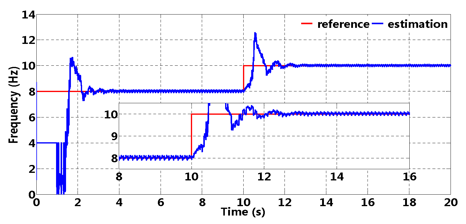
4. Fundamental Wave Frequency Estimation

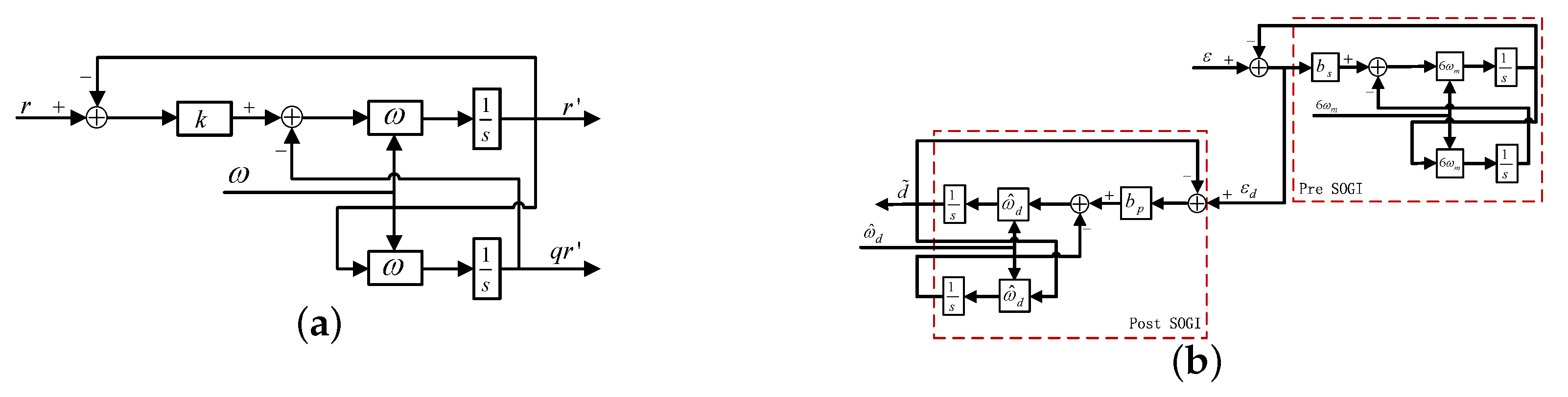
As stated in Section 2, periodic load disturbance is generally variable under different blue operating conditions. Central frequency of BPF can not regulate adaptively and fundamental wave component can not be extracted effectively; then, an adaptive SOGI observer is employed to extract fundamental wave component and fundamental wave frequency can be recursively estimated by the SM-ANF method.

4.1. SOGI Observer

The block diagram of SOGI is presented in Figure 14a, which can track or reject a certain frequency sinusoidal signal with insignificant error according to an internal model theorem. The block diagram of SOGI observer is presented in Figure 14b, which mainly consists of pre and post SOGI. Pre SOGI, being a band stop filter (BSF), is mainly employed to suppress $6$-th current harmonic brought about by the VSI nonlinear voltage drop. The gain waveforms of pre SOGI with respect to parameter $b_s$ are presented in Figure 15a; it can also be observed that the bandwidth of BSF becomes narrower with $b_s$ decreasing; however, smaller $b_s$ can slow down the response ratio; therefore, suppression performance and response ratio should be taken into consideration comprehensively when selecting $b_s$. Post SOGI is essentially a BPF, by selecting fundamental wave frequency as resonant frequency, which can filter off harmonic components effectively; in addition, constant quality factor ($1/b_p$) is convenient to extract a fundamental wave component from periodic disturbance, while the quality factor of general BPF is generally variable and determined by central frequency, bandwidth parameter, etc. The gain waveforms of post SOGI are presented in Figure 15b, and it is clear that $b_p$ decreases results in a remarkable narrowing of the pass band. When harmonic components are considerably abundant, a smaller $b_p$ can be preferred; however, a smaller $b_p$ can slow down the response ratio; therefore, it should achieve an optimal band pass characteristic between bandwidth and response ratio.

4.2. SM-ANF Method

Frequency estimation based on the SM-ANF method is presented in

Table 1. Frequency estimation based on SM-ANF method [33].

Input: m, $\Delta$, $\lambda$, ${\lambda }_r$, ${\lambda }_{\infty }$, $\rho$, ${\rho }_r$, ${\rho }_{\infty }$, $\mu$, $\delta$

Initialization: $\lambda =0.7$, ${\lambda }_r=0.99$, ${\lambda }_{\infty }=0.995$, $\delta =0.001$

$\rho =0.7$, ${\rho }_r=0.99$, ${\rho }_{\infty }=0.995$

$h\left(i\right)=g\left(i\right)=0$ for $i=-2,\cdots ,-1$

Main loop:

$g\left(n\right)=\tilde{d}\left(n\right)-{\rho }^{2}g(n-2)-\rho g(n-1)\widehat{a}(n-1)$

$h\left(n\right)=\tilde{d}(n-\Delta )-{\rho }^{2}h(n-2)-\rho h(n-1)\widehat{a}(n-1)$

$\varphi \left(n\right)=-\rho g(n-\Delta )+(\rho -1)h\left(n\right)$

Adaptive algorithm:

$e\left(n\right)=g(n-\Delta +1)+{\rho }^{2}g(n-\Delta -1)-({\rho }^2-1)h(n-1)-\varphi \left(n\right)\widehat{\theta }(n-1)$

$\widehat{\theta }\left(n\right)=\widehat{\theta }(n-1)+\frac{\mu }{\delta +\varphi \left(n\right)\varphi \left(n\right)}\varphi \left(n\right)e\left(n\right)$

$\lambda ={\lambda }_r\lambda +(1-{\lambda }_r){\lambda }_{\infty }$

$\rho ={\rho }_r\rho +(1-{\rho }_r){\rho }_{\infty }$

Fundamental frequency:

${\widehat{\omega }}_d\left(n\right)={cos}^{-1}(-0.5\widehat{\theta }\left(n\right))/T_s$

. $\Delta$ represents a delay parameter which is employed to attenuate the correlation between $h\left(n\right)$ and $g\left(n\right)$ contaminated by colored noise; $\lambda$, generally referred to as forgetting factor, increases at each iteration from initial value toward ${\lambda }_{\infty }$ at geometric ratio ${\lambda }_r$; similarly, $\rho$, generally referred to as bandwidth of ANF, increases in the same way from the initial value toward ${\rho }_{\infty }$ at geometric ratio ${\rho }_r$, the closer the parameter is to the unit, the narrower is the notch bandwidth; Newton least mean square (Newton-LMS) is substituted by normalized LMS (NLMS) to reduce computational complexity [38]; regular parameter $\delta$ is introduced to avoid numerical divergence in matrix inversion; $\mu$, $0<\mu ⩽1$, being the step size of NLMS, determines frequency estimation convergence ratio.

Parameters $\Delta$ and $g_a$ should be taken into consideration during fundamental frequency estimation. In order to optimize frequency estimation, frequency estimation based on the SM-ANF method is provided and reference frequency is presented in Equation (21).

$${\omega }_0\left(t\right)=\left\{\begin{array}{cc}\hfill 1.5\mathrm{rad}/\mathrm{s}& 0<t⩽6\mathrm{s}\hfill \\ \hfill 2\mathrm{rad}/\mathrm{s}& 6<t⩽20\mathrm{s}\hfill \end{array}\right.$$

(21)

Colored noise with signal noise ratio (SNR) 1/0.04 can be acquired through a AR(1) (auto-regression) model with transfer function $1/(1-0.8z^{-1})$. The effectiveness of delay parameter on frequency estimation is presented in Figure 16a. It can be observed that, for $\Delta =4$, frequency estimation deviation is introduced by the correlation between $h\left(n\right)$ and $g\left(n\right)$, for $\Delta =15$, weak correlation between $h\left(n\right)$ and $g\left(n\right)$ improves frequency estimation precision. In addition, when reference frequency suddenly changes, frequency estimation can realize fast tracking without great overshoot. Consequently, a proper delay parameter can reduce correlation to improve frequency estimation precision.

$q_a\left(e^{-j\omega T_s}\right)=g_a/(j\omega +g_a)$ with cut-off frequency $g_a$ is adopted to smooth frequency estimation and avoid possible overshoot. As presented in Figure 16b, it can be observed that, for $g_a=30\mathrm{rad}/\mathrm{s}$, frequency estimation has great overshoot in the beginning, and it takes 2 s to track the reference frequency; however, for $g_a=5\mathrm{rad}/\mathrm{s}$, frequency estimation waveform becomes smooth without great overshoot in the beginning and frequency sudden change. Consequently, an appropriate selection of cut-off frequency $g_a$ can smooth frequency estimation and avoid possible overshoot.

5. Simulations and Experiments

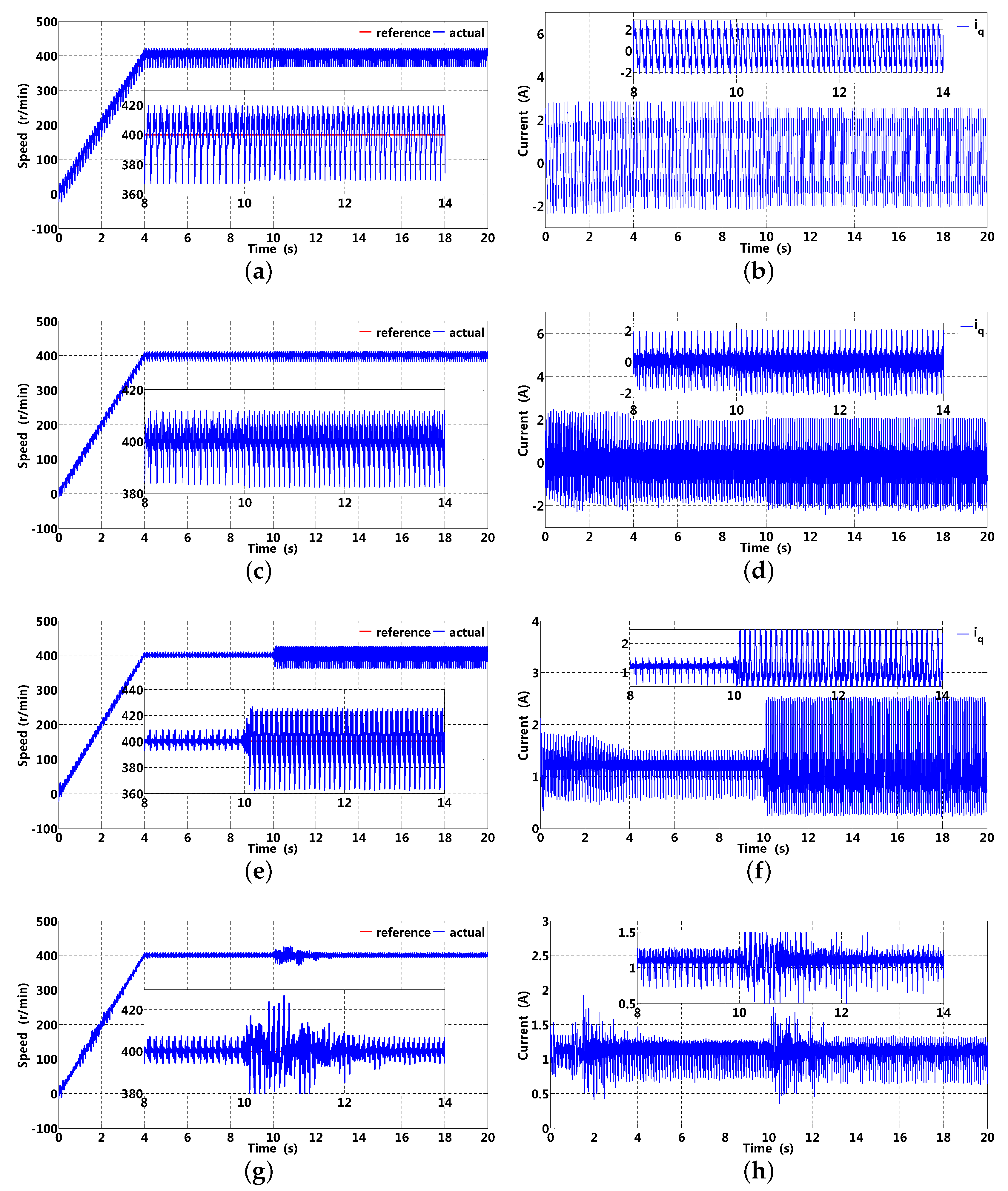
5.1. Simulation Analysis

Fundamental frequency estimation of periodic disturbance is critical to implement adaptive RRC (ARRC) analyzed above. In order to demonstrate the feasibility and effectiveness of ARRC, speed fluctuation suppression based on an original PI controller (without disturbance compensation), general DOB (the control scheme is presented in Figure 3b, RRC, and ARRC are constructed, respectively; in addition, the corresponding $q$-axis current is provided.

The simulation parameters are presented in

Table 2. Simulation parameters.

Parameter	Symbol	Value
Sampling time	$T_s$	0.1 $\mathrm{ms}$
Cut-off frequency of general DOB	$g_{dob}$	800 $\mathrm{rad}/\mathrm{s}$
Cut-off frequency of $q_c\left(z^{-1}\right)$	$g_c$	800 $\mathrm{rad}/\mathrm{s}$
Cut-off frequency of $q_a\left(z^{-1}\right)$	$g_a$	10 $\mathrm{rad}/\mathrm{s}$
Delay parameter	$\Delta$	15
Parameter of post SOGI	$b_p$	0.1
Parameter of pre SOGI	$b_s$	0.1
S-G filter order	p	3
Design parameter	D	2.6
Gain of RRC	$K_q$	0.6
Step size of NLMS	$\mu$	0.3
Stator winding resistance	$R_s$	2.875 $\Omega$
$d$-axis inductance	$L_d$	0.0085 $\mathrm{H}$
$q$-axis inductance	$L_q$	0.0119 $\mathrm{H}$
Rotor permanent magnetic flux	${\varphi }_m$	0.175 $\mathrm{Wb}$
Moment of inertia	$J_n$	0.003$\mathrm{kg}·{\mathrm{m}}^2$
Pole pairs	$n_p$	3
Electro-magnetic torque constant	$K_{Tn}$	0.525$\mathrm{Nm}/\mathrm{A}$
DC bus voltage	$V_{dc}$	310$\mathrm{V}$
Rated current	I	7 A

, where 400 r/min (20 Hz) is selected as reference value; in addition, fundamental frequency and periodic disturbance (including fundamental and harmonic components) are provided as follows:

$$f_0=\left\{\begin{array}{cc}\hfill 8\mathrm{Hz}& 0<t⩽10\mathrm{s}\hfill \\ \hfill 10\mathrm{Hz}& 10<t⩽20\mathrm{s}\hfill \end{array}\right.,\left\{\begin{array}{cc}\hfill A_p& =\left[\begin{array}{cccccc}1& 0.2& 0.3& 0.4& 0.6& 0.1\end{array}\right]\hfill \\ \hfill d_p& =\sum _{n=1}^6{A}_p\left[n\right]sin\left(n{f}_{0}t\right)\hfill \end{array}\right.$$

(22)

The speed and corresponding $q$-axis current based on an original PI controller (without $q$-axis current compensation), general DOB, RRC, and ARRC are presented in Figure 17, where the left and right show speed and corresponding $q$-axis current, respectively. Speed and corresponding $q$-axis current with the original PI controller are presented in Figure 17a,b, and it can be observed that speed has obvious fluctuation; in addition, $q$-axis current has periodic fluctuation which is primarily brought about by periodic load disturbance. Speed and corresponding $q$-axis current with DOB are presented in Figure 17c,d, and all disturbance components (including periodic and aperiodic) within the cut-off frequency can be employed for $q$-axis current compensation, although speed fluctuation can be suppressed to some extent (no more than 20 r/min), and a small sensitivity gain at disturbance related frequencies can not further enhance speed fluctuation suppression performance. Speed and corresponding $q$-axis current with RRC are presented in Figure 17e,f, and it can be observed that speed fluctuation can be effectively suppressed before fundamental frequency variation; however, RRC lacks frequency adaptiveness results in apparent speed fluctuation after fundamental frequency variation. The speed and corresponding $q$-axis current with ARRC are presented in Figure 17g,h, and apparent speed fluctuation in a transient stage (speed up), owing to frequency estimation deviation, takes almost 4 s to recover its steady state; in addition, it has small speed fluctuation (no more than 10 r/min), and a similar situation can exist when fundamental frequency changes suddenly. From the analyses mentioned above, speed fluctuation can be effectively suppressed with ARRC owing to sufficient sensitivity gain at fundamental and harmonic frequencies compared to that of DOB; meanwhile, an RRC lack of frequency adaptiveness may cause speed fluctuation suppression performance to deteriorate after fundamental frequency variation. Therefore, speed fluctuation brought about by periodic disturbance can be effectively suppressed by ARRC, while RRC can not.

Fundamental wave frequency estimation is presented in Figure 18 and 4 Hz is selected as initial value. It can be observed that frequency estimation value remains constant in the beginning, which illustrates that any sinusoidal component can not be extracted and then 4 Hz is still selected as estimation value; however, frequency estimation value can fast track reference value by adaptive regulation. When reference frequency varies suddenly, frequency estimation can track reference value with small overshoot and short adjusting time (no more than 3 s); in addition, high estimation accuracy in the steady state (no more than 0.15 Hz) can satisfy with practical application requirement, which can build a solid foundation for ARRC implementation.

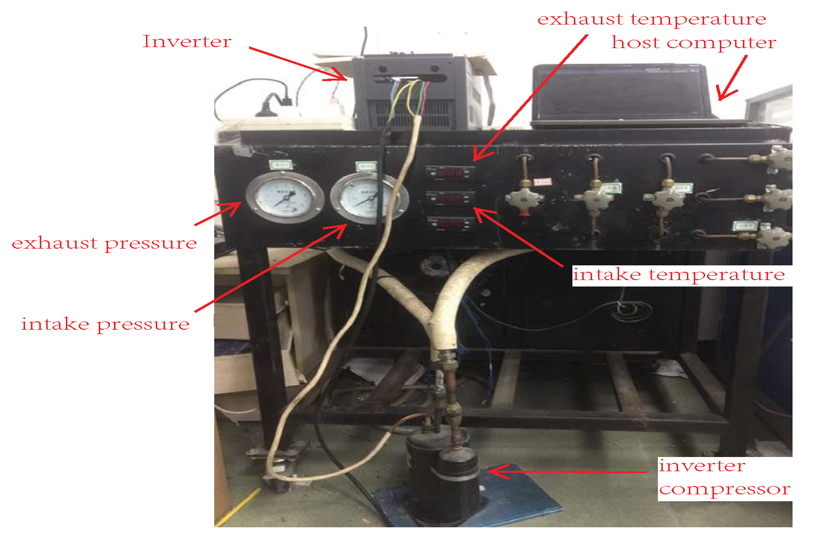
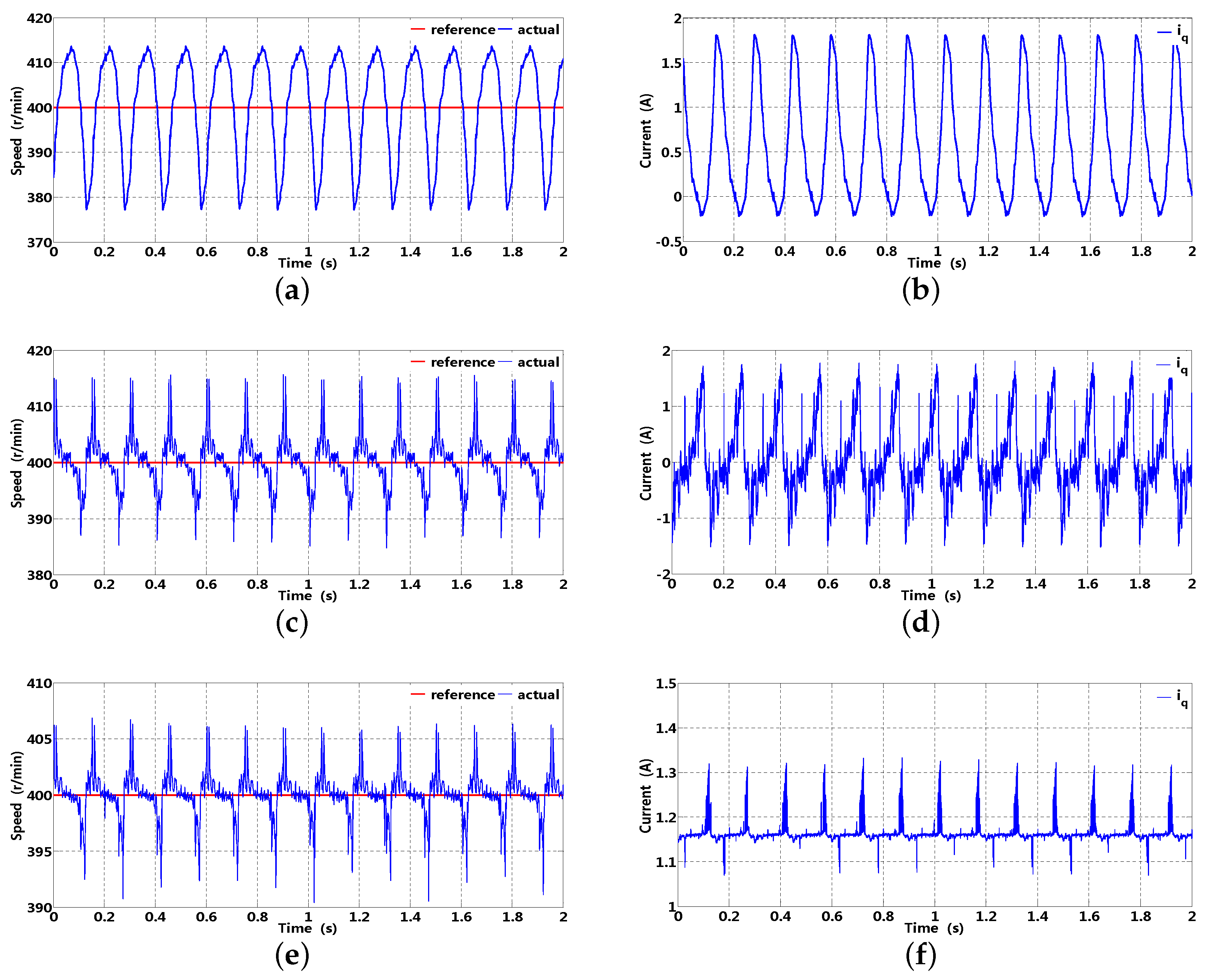
5.2. Experiment Setup

The nominal parameters of inverter compressor are presented in

Table 3. Experimental parameters.

Parameter	Symbol	Value
Pole pairs	$n_p$	3
Stator winding resistance	R	1.47 $\Omega$
$d$-axis inductance	$L_d$	6.87 mH
$q$-axis inductance	$L_q$	9.31 mH
Rotor permanent magnetic flux	${\varphi }_m$	345 mWb
Back electromotive force (BEMF) constant	$K_v$	39.2 V/krpm
Electro-magnetic torque constant	$K_T$	0.46 Nm/A
Moment of inertia	J	310 Kg·mm${}^2$
Rated current	$I_n$	5.2 A
Rated frequency	$f_n$	60 Hz
Cut-off frequency of general DOB	$g_{dob}$	800 $\mathrm{rad}/\mathrm{s}$
Cut-off frequency of $q_c\left(z^{-1}\right)$	$g_c$	800 $\mathrm{rad}/\mathrm{s}$
Cut-off frequency of $q_a\left(z^{-1}\right)$	$g_a$	10 $\mathrm{rad}/\mathrm{s}$
Delay parameter	$\Delta$	15
Parameter of post SOGI	$b_s$	0.1
Parameter of pre SOGI	$b_p$	0.1
S–G filter order	p	3
Step size of NLMS	$\mu$	0.3
Design parameter	D	2.6
Gain of RRC	$K_q$	0.6
Bandwidth of ANF	${\rho }_{init}$, ${\rho }_r$, ${\rho }_{\infty }$	0.8, 0.95, 0.99
Forgetting factor	${\lambda }_{init}$, ${\lambda }_r$, ${\lambda }_{\infty }$	0.8, 0.95, 0.99

. In order to validate effectiveness of the proposed scheme, experiments are implemented on inverter compressor platform presented in Figure 19, where digital signal processor (DSP) TMS320F28069 (TX) and IGBT module 7MBP50VFN060-50 are selected as a micro-processor and power device, respectively, sampling and pulse width modulation (PWM) switching frequency are selected as 10 KHz. Moreover, the current, voltage, and speed base value are selected as $5.2\times \sqrt{2}$$\mathrm{A}$, 310 $\mathrm{V}$ and 3000 $\mathrm{r}/\min$ (considering flux weakening range), respectively.

The speed and corresponding $q$-axis current at 20 Hz are presented in Figure 20, which can be real-time sampled and transferred to a host computer through a $\mathrm{CAN}–\mathrm{USB}$ converter; in addition, the suction and exhaust pressure are 0.3 and 1.5 Mpa, respectively, suction and exhaust temperature are 28 and $77{}^{°}$C, respectively. It is clear that speed has obvious fluctuation with an original PI controller (no more than 25 r/min); in addition, $q$-axis current presents a certain periodicity without compensation, which can possibly deteriorate normal operation of an inverter compressor. Although speed fluctuation can be suppressed to some extent with DOB, $q$-axis current periodicity in Figure 20d can not be effectively rejected, which may be brought about by the following reasons; firstly, periodic disturbance can not be effectively suppressed by the finite sensitivity gain of DOB; secondly, a small cut-off frequency of LPF can increase sensitivity gain; however, phase lag can deteriorate current compensation performance. The $q$-axis current harmonics brought about by periodic load disturbance can be effectively rejected in Figure 20f, except for some aperiodic components; in addition, smaller speed fluctuation can be obtained with ARRC (no more than 8 $\mathrm{r}/\min$). Under almost the same operating condition, there are similar situations at 25 Hz. In Figure 21a, speed fluctuation is obvious with the original PI controller (no more than 25 $\mathrm{r}/\min$); additionally, the $q$-axis current presents a certain periodicity without compensation. Similarly, speed suppression performance with DOB is unsatisfactory owing to its slightly smaller sensitivity gain. In Figure 21f, $q$-axis current harmonic disturbance can be effectively suppressed with ARRC; in addition, smaller speed fluctuation (no more than 5 $\mathrm{r}/\min$) can be obtained compared to that of DOB (no more than 12 $\mathrm{r}/\min$).

In order to reflect speed fluctuation suppression performance intuitively, speed fluctuation ratio ${\rho }_{spd}$ is introduced based on root mean square error (RMSE) criterion, which can be expressed as follows:

$$\begin{array}{c}\hfill {\rho }_{spd}=\sqrt{\frac{1}{N_c}{\displaystyle \sum _{i=1}^{N_c}}{\left(\frac{{\omega }_m\left(i\right)}{{\omega }_m^{*}}-1\right)}^2}\end{array}$$

(23)

where $N_c=n_p/\left(f{T}_{spd}\right)$, f, ${\omega }_m^{*}$ and ${\omega }_m$ represent sampling number, operation frequency, reference, and actual speed, respectively, $T_{spd}$ represents sampling time of speed loop and 1 $\mathrm{ms}$ is selected in this paper. The speed fluctuation ratio and its corresponding deviation are presented in

Table 4. Speed fluctuation ratio and its corresponding deviation.

Method	20 Hz	25 Hz
PI	2.92%	1.83%
	11.7 r/min	9.2 r/min
DOB	1.35%	0.94%
	5.4 r/min	4.7 r/min
ARRC	0.46%	0.34%
	1.8 r/min	1.7 r/min

. It can be observed that speed deviation is almost identical under almost the same operating condition, which corresponds with the assumption mentioned in Section 2; in addition, speed fluctuation ratio becomes larger with frequency decreasing under almost the same operating condition; on the contrary, comparably smaller speed fluctuation ratio can be obtained primarily owing to larger reference value, which illustrates that speed fluctuation in a low frequency range should be taken into consideration. Consequently, speed fluctuation suppression based on ARRC is feasible and effective in low frequency range for an inverter compressor.

6. Conclusions

In this paper, a revised repetitive control scheme has been proposed. Firstly, a novel S–G filter is constructed, its adjustable linear phase, and low pass characteristics can well approximate a disturbance delay element in a continuous domain; in addition, the principle of control scheme and S–G filter design method are provided. Secondly, the SOGI observer can be adopted to suppress specific frequency disturbance (pre SOGI) and extract fundamental component (post SOGI) from approximately periodic disturbance; furthermore, fundamental wave frequency is estimated based on SM-ANF and relevant parameters are analyzed and designed. Thirdly, MATLAB simulations and experiments are provided based on the original PI controller (without $q$-axis current compensation), DOB, and ARRC; results illustrate that speed fluctuation in a low frequency range can be effectively suppressed for the inverter compressor driving system. Furthermore, the paper can provide a novel idea for harmonics reduction in an active power filter system and photovoltaic inverter.

References

1. Zhang, G.Z. A Speed Fluctuation Method for Air Conditioner Compressor Based on Fourier Transformation. China Appl. 2013, S1, 491–496. [Google Scholar]
2. Huang, H.; Ma, Y.J.; Zhang, L.Y.; Mi, X.T. Method to Reduce the Speed Ripple of Single Rotator Compressor of Air Conditioner in Low Frequency. Electr. Mach. Control 2011, 15, 98–102. [Google Scholar]
3. Chen, W.H.; Yang, J.; Guo, L.; Li, S. Disturbance Observer-Based Control and Related Methods: An Overview. IEEE Trans. Ind. Electron. 2016, 63, 1083–1095. [Google Scholar] [CrossRef] [Green Version]
4. Yang, J.; Chen, W.H.; Li, S.H.; Guo, L.; Yan, Y. Disturbance/Uncertainty Estimation and Attenuation Techniques in PMSM Drives—A Survey. IEEE Trans. Ind. Electron. 2016, 64, 3273–3285. [Google Scholar] [CrossRef] [Green Version]
5. Ohnishi, K.; Shibata, M.; Murakami, T. Motion control for advanced mechatronics. IEEE-ASME Trans. Mechatron. 2002, 1, 56–67. [Google Scholar] [CrossRef]
6. Huang, Y.; Xue, W.C. Active disturbance rejection control: Methodology, application and theoretical analysis. ISA Trans. 2014, 53, 963–976. [Google Scholar] [CrossRef]
7. Fei, Q.; Deng, Y.T.; Li, H.W.; Liu, J.; Shao, M. Speed Ripple Minimization of Permanent Magnet Synchronous Motor Based on Model Predictive and Iterative Learning Controls. IEEE Access 2019, 34, 31791–31800. [Google Scholar] [CrossRef]
8. Qian, W.Z.; Panda, S.K.; Xu, J.X. Torque ripple minimization in PM synchronous motors using iterative learning control. IEEE Trans. Power Electron. 2004, 19, 272–279. [Google Scholar] [CrossRef]
9. Kuang, Z.; Du, B.C.; Cui, S.M.; Chan, C.C. Speed Control of Load Torque Feedforward Compensation Based on Linear Active Disturbance Rejection for Five-Phase PMSM. IEEE Access 2019, 7, 159787–159796. [Google Scholar] [CrossRef]
10. Lu, E.; Li, W.; Yang, X.F.; Liu, Y. Anti-disturbance speed control of low-speed high-torque PMSM based on second-order non-singular terminal sliding mode load observer. ISA Trans. 2018, 88, 142–152. [Google Scholar] [CrossRef]
11. Xu, W.; Junejo, A.K.; Liu, Y.; Rabiul Islam, M. Improved Continuous Fast Terminal Sliding Mode Control with Extended State Observer for Speed Regulation of PMSM Drive System. IEEE Trans. Veh. Technol. 2019, 68, 10465–10476. [Google Scholar] [CrossRef]
12. Deng, Y.T.; Wang, J.L.; Li, H.W.; Liu, J.; Tian, D. Adaptive sliding mode current control with sliding mode disturbance observer for PMSM drives. ISA Trans. 2018, 82, 113–126. [Google Scholar] [CrossRef] [PubMed]
13. Hara, S.; Yamamoto, Y.; Omata, M.; Nakano, M. Repetitive control system: A new type servo system for periodic exogenous signals. IEEE Trans. Autom. Control 1988, 33, 659–668. [Google Scholar] [CrossRef] [Green Version]
14. Francis, B.A.; Wonham, W.M. The internal model principle for linear multivariable regulators. Appl. Math. Optim. 1975, 2, 170–194. [Google Scholar] [CrossRef]
15. Chen, X.; Tomizuka, M. New Repetitive Control With Improved Steady-State Performance and Accelerated Transient. IEEE Trans. Control Syst. Technol. 2014, 22, 664–675. [Google Scholar] [CrossRef]
16. Pipeleers, G.; Demeulenaere, B.; De Schutter, J.; Swevers, J. Robust high-order repetitive control: Optimal performance trade-offs. Automatica 2008, 44, 2628–2634. [Google Scholar] [CrossRef]
17. Weiss, G.; Hafele, M. Repetitive control of MIMO systems using H design. Automatic 1999, 35, 1185–1199. [Google Scholar] [CrossRef]
18. Jiang, S.; Cao, D.; Peng, F.Z.; Li, Y.; Liu, J. Low THD, fast transient, and cost-effective synchronous-frame repetitive controller for three-phase UPS inverters. IEEE Trans. Power Electron. 2012, 27, 2819–2826. [Google Scholar] [CrossRef]
19. Zou, Z.X.; Zhou, K.L.; Wang, Z.; Cheng, M. Frequency-Adaptive Fractional-Order Repetitive Control of Shunt Active Power Filters. IEEE Trans. Ind. Electron. 2015, 62, 1659–1668. [Google Scholar] [CrossRef]
20. Lu, Y.S.; Lin, S.M.; Hauschild, M.; Hirzinger, G. A torque-ripple compensation scheme for harmonic drive systems. Electr. Eng. 2013, 95, 357–365. [Google Scholar] [CrossRef]
21. Tang, Z.Y.; Akin, B. Suppression of Dead-Time Distortion Through Revised Repetitive Controller in PMSM Drives. IEEE Trans. Energy Convers. 2017, 32, 918–930. [Google Scholar] [CrossRef]
22. Mattavelli, P.; Tubiana, L.; Zigliotto, M. Torque-ripple reduction in PM synchronous motor drives using repetitive current control. IEEE Trans. Power Electron. 2005, 20, 1423–1431. [Google Scholar] [CrossRef]
23. Zhang, B.; Zhou, K.L.; Wang, Y.G.; Wang, D. Performance improvement of repetitive controlled PWM inverters: A phase-lead compensation solution. Int. J. Circuit Theory Appl. 2010, 38, 453–469. [Google Scholar] [CrossRef]
24. Cui, P.L.; Li, S.; Zhao, G.Z.; Peng, C. Suppression of Harmonic Current in Active-Passive Magnetically Suspended CMG Using Improved Repetitive Controller. IEEE-ASME Trans. Mechatron. 2016, 21, 2132–2141. [Google Scholar] [CrossRef]
25. Cao, Z.W.; Ledwich, G.F. Adaptive repetitive control to track variable periodic signals with fixed sampling rate. IEEE-ASME Trans. Mechatron. 2002, 7, 378–384. [Google Scholar]
26. Weiss, G.; Zhong, Q.C.; Green, T.C.; Liang, J. H repetitive control of DC-AC converters in microgrids. IEEE Trans. Power Electron. 2004, 19, 219–230. [Google Scholar] [CrossRef]
27. Hornik, T.; Zhong, Q.C. H repetitive voltage control of gridconnected inverters with a frequency adaptive mechanism. IET Power Electron. 2010, 3, 925–935. [Google Scholar] [CrossRef]
28. Chen, D.; Zhang, J.M.; Qian, Z.M. An Improved Repetitive Control Scheme for Grid-Connected Inverter With Frequency-Adaptive Capability. IEEE Trans. Ind. Electron. 2013, 60, 814–823. [Google Scholar] [CrossRef]
29. Chen, D.; Zhang, J.M.; Qian, Z.M. Research on fast transient and 6n ± 1 harmonics suppressing repetitive control scheme for three-phase grid-connected inverters. IET Power Electron. 2013, 6, 601–610. [Google Scholar] [CrossRef]
30. Marino, R.; Tomei, P. Adaptive notch filters are local adaptive observers. Int. J. Adapt. Control Signal Process. 2015, 30, 128–146. [Google Scholar] [CrossRef]
31. Li, G. A stable and efficient adaptive notch filter for direct frequency estimation. IEEE Trans. Signal Process. 1997, 45, 2001–2009. [Google Scholar]
32. Cheng, M.H.; Tsai, J.L. A new IIR adaptive notch filter. Signal Process. 2006, 86, 1648–1655. [Google Scholar] [CrossRef]
33. Sariyildiz, E.; Ohnishi, K. Stability and Robustness of Disturbance-Observer-Based Motion Control Systems. IEEE Trans. Ind. Electron. 2014, 62, 414–422. [Google Scholar] [CrossRef]
34. Muramatsu, H.; Katsura, S. Adaptive Periodic-Disturbance Observer for Periodic-Disturbance Suppression. IEEE Trans. Ind. Inform. 2018, 14, 4446–4456. [Google Scholar] [CrossRef]
35. William, A.B.; Taylor, F.J. Electronic Filter Design Handbook; McGraw-Hill: New York, NY, USA, 2006; pp. 566–570. [Google Scholar]
36. Saeid, J.; Ioannou, P.A.; Ben, I.; Wang, Y. Robustness and Performance of Adaptive Suppression of Unknown Periodic Disturbances. IEEE Trans. Autom. Control 2015, 60, 2166–2171. [Google Scholar]
37. Wu, X.H.; Panda, S.K.; Xu, J.X. Design of a Plug-In Repetitive Control Scheme for Eliminating Supply-Side Current Harmonics of Three-Phase PWM Boost Rectifiers Under Generalized Supply Voltage Conditions. IEEE Trans. Power Electron. 2010, 25, 1800–1810. [Google Scholar] [CrossRef]
38. Sayed, A.H. Adaptive Filters; John Wiley & Sons Inc.: Hoboken, NJ, USA, 2008; pp. 187–193. [Google Scholar]
Figure 1. Structural diagram of inverter compressor and operation cycle: (a) inverter compressor structure; (b) stator winding and bump; (c) refrigeration loop of air-conditioner.
Energies 13 06342 g001
Figure 2. Load torque under different operating conditions.
Energies 13 06342 g002
Figure 3. Equivalent control block diagram of inverter compressor: (a) FOC; (b) FOC with general DOB.
Energies 13 06342 g003
Figure 4. Structural diagram of repetitive controller in discrete domain: (a) IRC; (b) RRC.
Energies 13 06342 g004
Figure 5. Block diagram of disturbance internal model: (a) continuous domain; (b) discrete domain.
Energies 13 06342 g005
Figure 6. Gain and phase waveforms of IRC and RRC, where corresponding parameters are N = 1044 , ω 0 = 60 rad/s, K q = 0.6 , D = 2.6 and T s = 0.1 ms. (a) gain; (b) phase.
Energies 13 06342 g006
Figure 7. Block diagram of FOC with RRC: (a) general; (b) adaptive.
Energies 13 06342 g007
Figure 8. Gain and phase waveforms of q -axis current open-loop transfer function, where corresponding parameters are N = 1044 , ω 0 = 60 rad/s, p = 3 , D = 2.6 and T s = 0.1 ms, respectively. (a) gain; (b) phase.
Energies 13 06342 g008
Figure 9. Gain waveforms of q -axis open-loop transfer function with respect to parameter p and K q , where corresponding parameters are N = 1044 , ω 0 = 60 rad/s, D = 2.6 and T s = 0.1 ms, respectively. (a) parameter p; (b) parameter K q .
Energies 13 06342 g009
Figure 10. Gain and phase waveforms of q -axis current sensitivity function, where corresponding parameters are N = 1044 , ω 0 = 60 rad/s, K q = 0.6 , p = 3 , D = 2.6 and T s = 0.1 ms, respectively. (a) gain; (b) phase.
Energies 13 06342 g010
Figure 11. Gain and phase waveforms of q -axis complementary sensitivity function, where corresponding parameters are N = 1044 , ω 0 = 60 rad/s, K q = 0.6 , p = 3 , D = 2.6 and T s = 0.1 ms, respectively. (a) gain; (b) phase.
Energies 13 06342 g011
Figure 12. Gain and phase waveforms of q -axis sensitivity function with respect to resistance variation, where corresponding parameters are N = 1044 , ω 0 = 60 rad/s, K q = 0.6 , p = 3 , D = 2.6 and T s = 0.1 ms, respectively. (a) R s ; (b) 2 R s .
Energies 13 06342 g012
Figure 13. Gain and phase waveforms of q -axis sensitivity function with respect to inductance variation, where corresponding parameters are N = 1044 , ω 0 = 60 rad/s, K q = 0.6 , p = 3 , D = 2.6 and T s = 0.1 ms, respectively. (a) L q ; (b) 2 L q .
Energies 13 06342 g013
Figure 14. Block diagram of SOGI. (a) general SOGI; (b) pre and post SOGI.
Energies 13 06342 g014
Figure 15. Gain waveforms with respect to parameter b s and b p , where corresponding parameters are ω 0 = 100 rad/s and T s = 0.1 ms, respectively. (a) pre SOGI; (b) post SOGI.
Energies 13 06342 g015
Figure 16. Frequency estimation with respect to parameter Δ and g a . (a) Δ ; (b) g a .
Energies 13 06342 g016
Figure 17. Speed and corresponding q -axis current based on original PI controller (without q -axis current compensation), DOB, RRC, and ARRC. (a,b) speed and corresponding q -axis current with an original PI controller; (c,d) speed and corresponding q -axis current with DOB; (e,f) speed and corresponding q -axis current with RRC; (g,h) speed and corresponding q -axis current with ARRC.
Energies 13 06342 g017
Figure 18. Fundamental frequency estimation.
Energies 13 06342 g018
Figure 19. Experimental platform of an inverter compressor driving system.
Energies 13 06342 g019
Figure 20. Speed and corresponding q -axis current based on original PI controller (without q -axis current compensation), DOB and ARRC (20 Hz): (a,b) speed and corresponding q -axis current with an original PI controller; (c,d) speed and corresponding q -axis current with DOB; (e,f) speed and corresponding q -axis current with ARRC.
Energies 13 06342 g020
Figure 21. Speed and corresponding q -axis current based on original PI controller (without q -axis current compensation), DOB and ARRC (25 Hz). (a,b) speed and corresponding q -axis current with original PI controller; (c,d) speed and corresponding q -axis current with DOB; (e,f) speed and corresponding q -axis current with ARRC.
Energies 13 06342 g021