Review

Review of Methods Used for Selecting Pumps as Turbines (PATs) and Predicting Their Characteristic Curves

Department of Mechanical, Energy and Management Engineering, University of Calabria, Ponte Bucci, Cube 44C, 87036 Rende, Italy
*
Author to whom correspondence should be addressed.
Energies 2020, 13(23), 6341; https://doi.org/10.3390/en13236341
Submission received: 8 November 2020 / Revised: 24 November 2020 / Accepted: 27 November 2020 / Published: 1 December 2020

Abstract

:
The use of Pumps As Turbines (PATs) can be the best solution for exploiting small hydraulic resources. Pump manufacturers do not provide the performances of their machines running in reverse mode, thus several authors developed appropriate prediction models. Some of them can only correlate the pump Best Efficiency Point (BEP) to the PAT corresponding one; other ones are able to obtain the characteristic curves. In this paper, a review of these methodologies is presented with the aim to find the best strategy that allows a designer of a small hydropower plant to select the PAT to be used and to predict its characteristic curves. The study also highlights the possibility of disassembling some models in order to merge the best parts in a more reliable strategy.

1. Introduction

Pumps running in reverse mode, Pumps As Turbines (PATs), can be effectively used for exploiting small hydraulic resources, with the main advantage of being cheaper than traditional hydraulic turbines [1]. Other favorable aspects can be found in the wide presence of pump manufacturers all around the world, with spare parts easily available. Moreover, pumps are technologically simpler than hydraulic turbines, thanks to the lack of a flow control system [1].
PATs can be found in different plants with the aim of producing electrical energy, for example reverse-running pumps can substitute Pressure Reducing Valves (PRVs) in Water Distribution Networks (WDNs), as reported by various authors [2,3,4,5,6,7,8].
Among the several researchers, Patelis et al. [2] analyzed three different scenarios in the WDN of Kozani city, considering a case without pressure adjusting, one with PRVs and another one with PATs. Even if pressure control is better with PRVs, the result of the study was favorable to the use of PATs because, in parallel to pressure reducing, it is possible to recover energy that can be used for the network needs.
Meirelles Lima et al. [3] developed an optimization procedure for selecting the PAT to be installed substituting a PRV in water distribution networks. In particular, the authors proposed a particle swarm optimization able to maximize energy production and volume leakage reductions, taking into account the constraints given by pressure limits in the nodes. Applying the procedure to a case study Meirelles Lima et al. [3] once again highlighted that pressure reducing valves provide a better pressure regulation compared to reverse-running pumps, but PATs guarantee energy recovery and a potential economic benefit.
Alberizzi et al. [4] analyzed the possibility of using variable-speed PATs in WDNs by means of a model created using MATLAB® Simulink. The authors highlighted that, in the condition of the same PAT downstream pressure, the use of a variable-speed PAT can result in a 23% increase of energy recovered in comparison to the case without control system.
In irrigation systems, PRVs are also present for pressure control and can be substituted with PATs, as studied by Algieri et al. [9]. The authors proposed a new method for selecting the PAT to be installed as well as a multi-variable optimization to obtain the best hydropower plant configuration. Moreover, Algieri at al. [9] identified 114 potential hydropower plants in the irrigation systems present in Calabria (Southern Italy). This solution does not just provide energy to be used by irrigation systems themselves but can lead to reduced greenhouse gases emissions.
PATs can also be used in industrial plants such as oil refineries, as analyzed by Renzi et al. [10], in which the wastewater is discharged to the sea by gravity, after the necessary treatments. Furthermore, it is possible to recover energy from rainwater, as described by Barbarelli et al. [11], using an underground storage tank alongside a PAT, creating a solution perfectly integrated with the evolution of smart grids.
Furthermore, it is possible to use PATs in Pumped-Hydro Energy Storage (PHES) systems, not only in high power plants, but also in micro-hydropower ones [12,13].
Renewable energy sources can be the best solution in order to meet the need for electricity in developing countries and hydraulic energy is the one characterized by the lowest cost [14]. Arriaga [15] studied the possibility of using a pico-hydropower plant to provide electrical energy in rural areas of Laos. The author compared different solutions to supply energy to offices and a village and highlighted the possibility of realizing a mini grid. Motwani et al. [16] proposed an economic analysis concerning a pico-hydropower plant in India, comparing the costs related to the PAT with the ones regarding a hydraulic turbine. The annual life cycle cost analysis carried out by the authors showed once again that using pumps running in reverse mode is convenient.
The main hindrance of using PATs is the lack of information related to their performances, which is not provided by pump manufacturers [1]. For this purpose, several authors developed models that belong to two main macro-approaches: Basic model that can correlate pump Best Efficiency Point (BEP) to the PAT one and models that can predict the characteristic curves of a PAT.
For exploiting small hydraulic resources using a PAT, two main problems arise: The selection of the PAT to be used and the prediction of the PAT characteristic curves. Concerning the first problem, basic models can be effectively used, starting from the hydraulic resource information [7,8]. The calculation of PAT characteristic curves requires more complex models and allows the identification of the operating point, necessary to estimate the producibility of the hydropower plant [7,8].
In this paper a review of the most important and recent methods used for predicting PAT performance is displayed, with the main objective of aiding the designer of hydroelectric plants suitable for the use of PAT. First, the various methods are briefly described focusing on the key points, then the study analyses their advantages and drawbacks. A global methodology has the aim of selecting the PAT, reconstruct the geometry and obtaining the characteristic curves. Even if various authors provided original contributions regarding these three modules, models could usually obtain good accuracy for a PAT, but are not able to work properly on another one. Therefore, in this paper the authors analyzed the possibility of disassembling the methods in modules and merge the best ones to create a new strategy with better reliability.

2. PAT Modeling Approaches

In order to obtain information about the performances of a PAT, appropriate methods have been developed by various researchers and can be found in the literature.
Several authors, listed in the following, proposed basic models that allow the most suitable PAT to be identified for a given site: Alatorre–Frenk [17], Algieri et al. [9], Barbarelli et al. [11], Childs [18], Derakhshan and Nourbakhsh [19], Grover [20], Hancock [21], Hergt [20], Sharma [20], Schmiedl [20], Stefanizzi [22], Stepanoff [20] and Yang et al. [23]. These methods are based on the calculation of two conversion factors CQ and CH expressed by Equations (1) and (2) [1].
C Q   =   Q BEPt Q BEPp
C H   =   H BEPt H BEPp
From the above equations, it is easy to observe that CQ is the ratio between PAT and pump flow rate at BEP, as well as CH is the ratio between PAT and pump head at BEP [1].
These two conversion factors can be used for the preliminary selection of the machine to be installed. In fact, knowing site flow rate Qsite = QBEPt and site head Hsite = HBEPt and calculating the conversion factors it is possible, by means of inverse formulas, to obtain QBEPp and HBEPp related to the pump and necessary to use the manufacturers’ catalogues [7,8].
Obtaining the characteristic curves of a PAT, is highly important to identify the operating point of the machine coupled with a given hydropower site. Methodologies that can predict the characteristic curves of a PAT can be classified as follows:
  • Empirical models
  • 1D models that recreate the unknown geometry of the machine
  • 1D models that use a known geometry
  • 2D models
  • 3D-CFD (Computational Fluid Dynamics) models
2D models are rare because the flow field is not characterized by particular symmetries and they are only cited in this paper. In fact, the hypothesis of a two-dimensional flux can be considered valid only for low specific speed turbomachines with radial flow [24]. Nevertheless, 2D models can be used for obtaining correlations that allow the slip factor to be calculated [25].

3. Basic Models

As discussed in the previous section, these models are based on the calculation of two conversion factors CQ and CH, usually expressed as a simple function of pump parameters (pump efficiency at BEP, ηBEPp and pump hydraulic efficiency at BEP, ηHBEP) or PAT parameters (PAT efficiency at BEP. ηBEPt and PAT specific speed, nst) [20,21]. These kinds of correlations are reported in Table 1.
The model proposed by Derakhshan and Nourbakhsh [19], in comparison to the other models, refers to the following parameters:
γ   =   ( C H ) 0.5 n t n p
α   =   n Q BEP ( gH BEP ) 0.75
β   =   n P BEP ρ 0.5 ( gH BEP ) 1.25
The parameter γ is necessary to calculate the head conversion factor CH, α is a dimensionless specific speed such as β, but the first is a function of the flow rate at BEP, while the latter is a function of power at BEP [19]. The authors proposed the following correlations based on the parameters above described [19]:
γ   =   0.0233   α p + 0.6464
α t   =   0.9413   α p 0.6045
β t   =   0.849   β p 1.2376
Moreover, it is worth observing that, among these basic models, only the methods developed by Alatorre–Frenk [17] and Barabrelli et al. [11] proposed a useful correlation to identify the value of PAT efficiency at BEP, respectively according to Equations (9) and (10).
η BEPt   =   η BEPp 0.03
η BEPt   =   0.00037 n st 2 + 0.02952 n st + 0.24326

4. Models that Predict the Characteristic Curves of a PAT

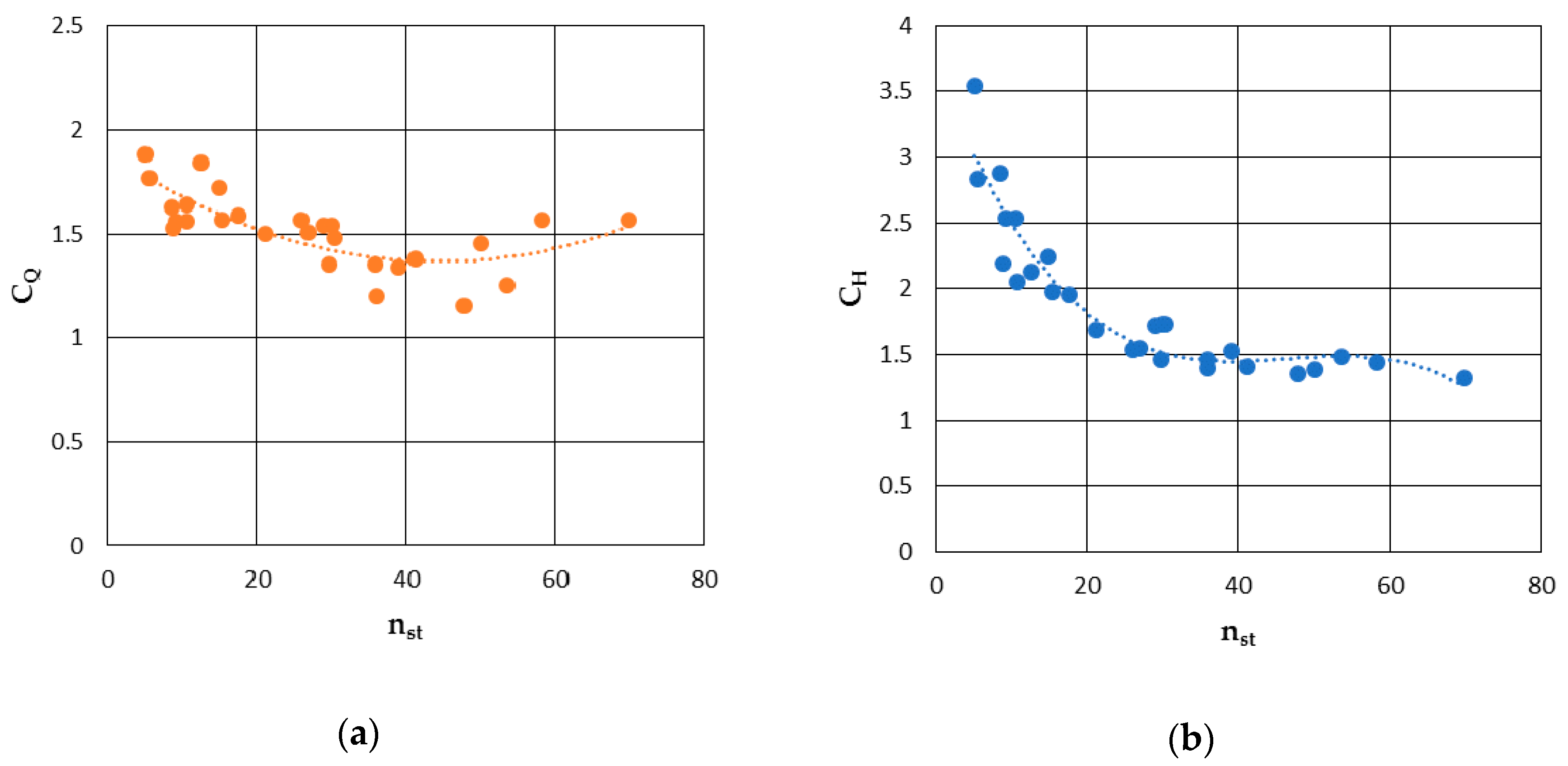
4.1. Empirical Models

Empirical models allow the characteristic curves of a reverse-running pump to be obtained using polynomials derived from a statistic analysis of experimental data, with the aim to have a universally valid method. In this study, the authors considered the method proposed by Derakhshan and Nourbakhsh [19] as representative of empirical models because, even if several authors [11,26] developed models of this typology, they are similar to each other. Experimental data regarding head and power as functions of flow rate can be excellently interpolated using polynomials of degree two and three, respectively. Even if these polynomial expressions are different according to various researchers, considering the dimensionless values of head, power and flow rate with respect to their values at BEP, the curves obtained are similar.

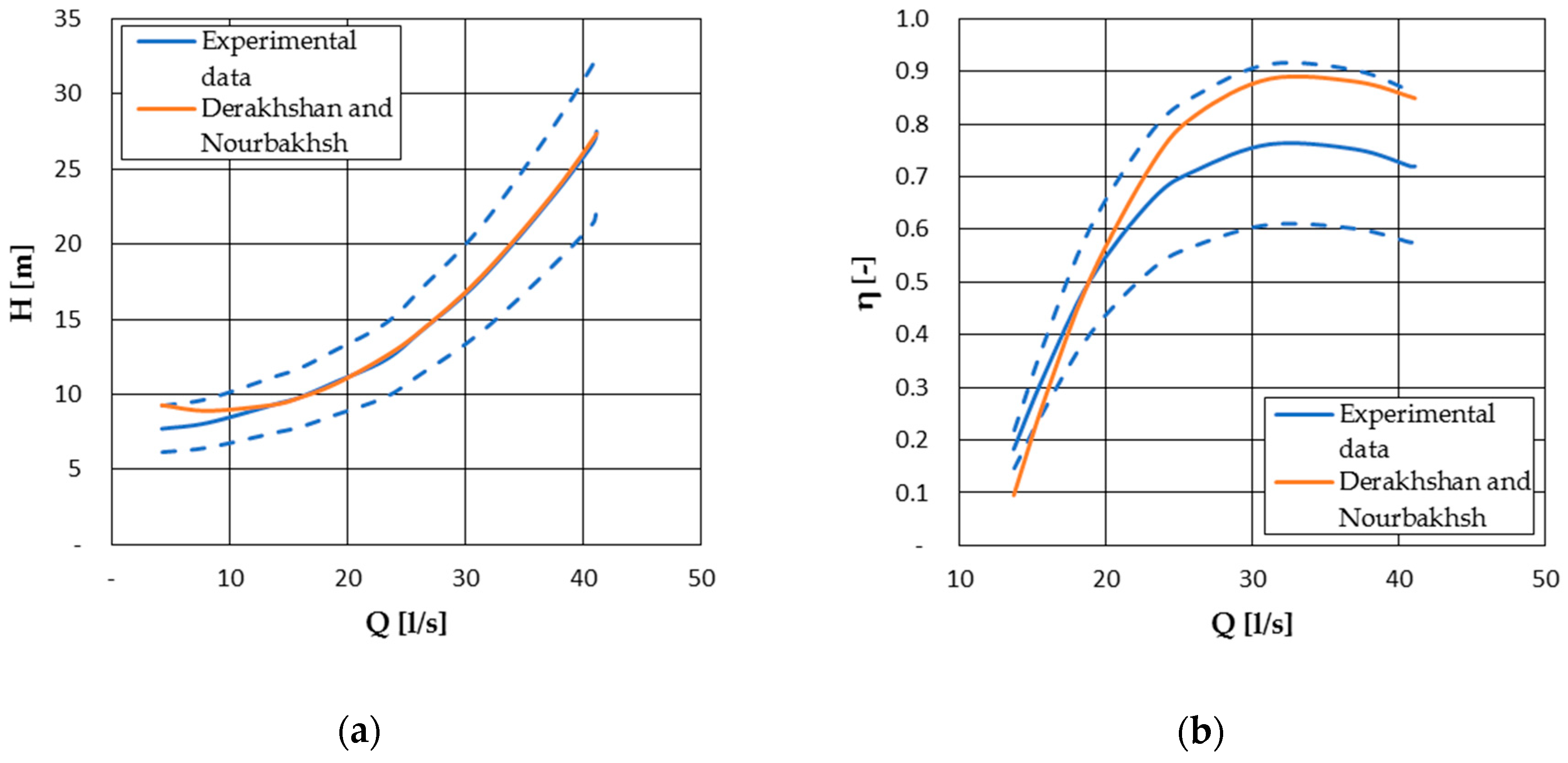
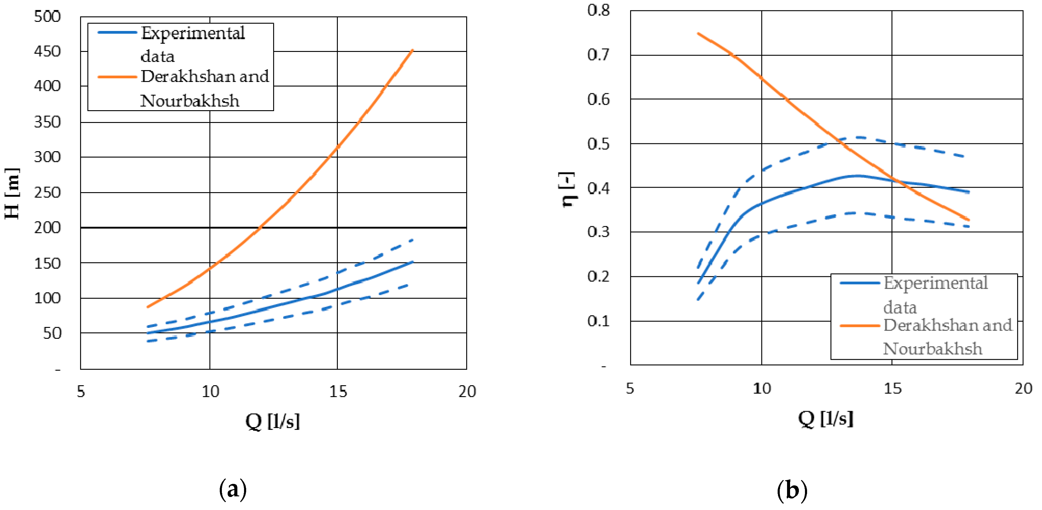
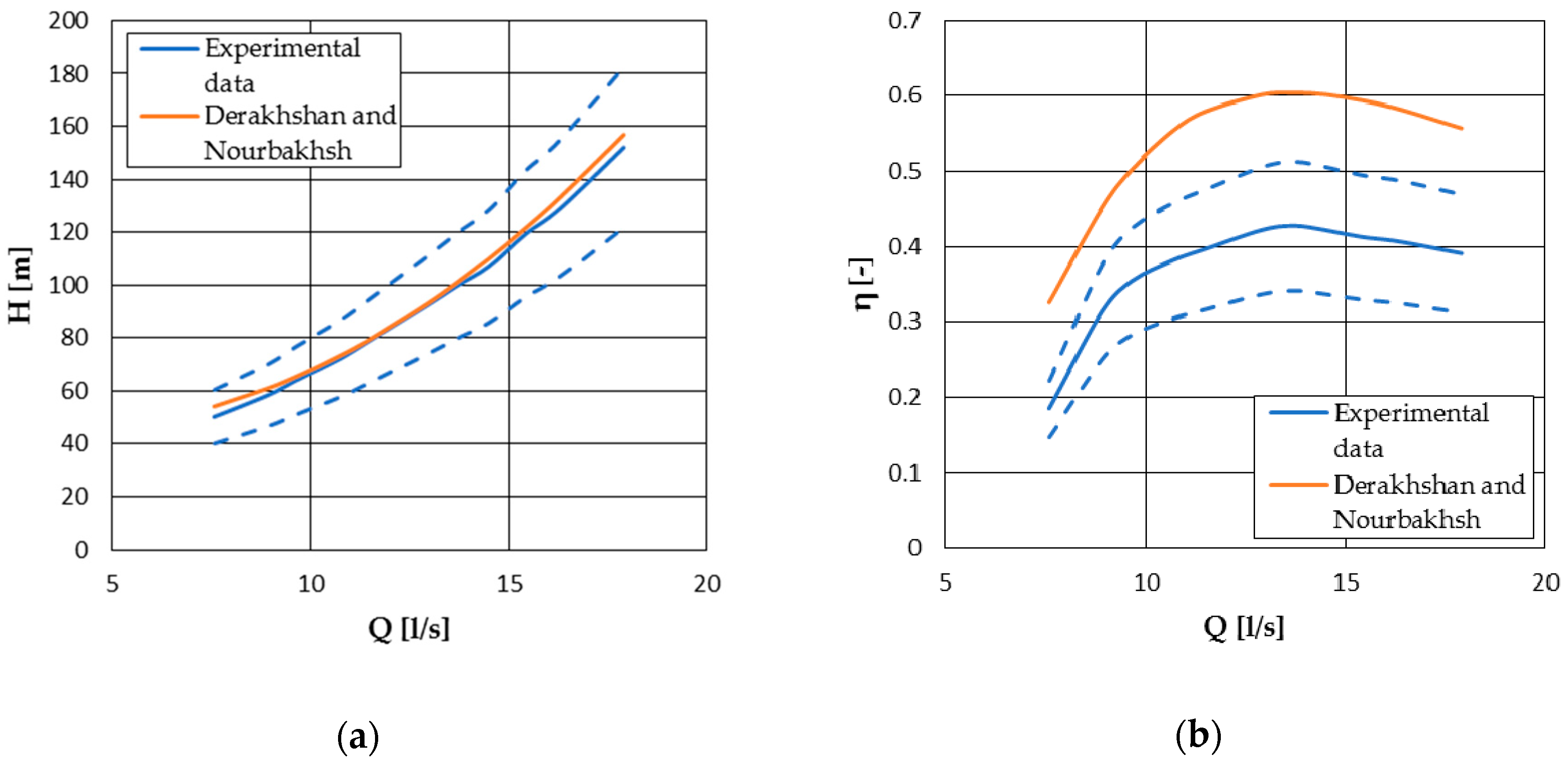
4.1.1. Derakhshan and Nourbakhsh Model

The methodology proposed by Derakhshan and Nourbakhsh [19] is based on experimental data obtained by the same authors testing four centrifugal pumps, using a purpose-made test rig. In particular, the specific speed of the machines selected is included in the range 14–56. The authors referred to dimensionless parameters for flow rate, head and power defined by Equation (11) [19].
q   =   Q t Q BEPt ;   h   =   H t H BEPt ;   p   =   P t P BEPt
The correlations proposed by Derakhshan and Nourbakhsh [19] to obtain the characteristic curves of a PAT are reported in the following equations:
h   =   1.0283   q 2 0.5468   q + 0.5314
p   =   0.3092   q 3 + 2.1472   q 2 0.8865   q + 0.0452
η t   =   P t ρ gH t Q t

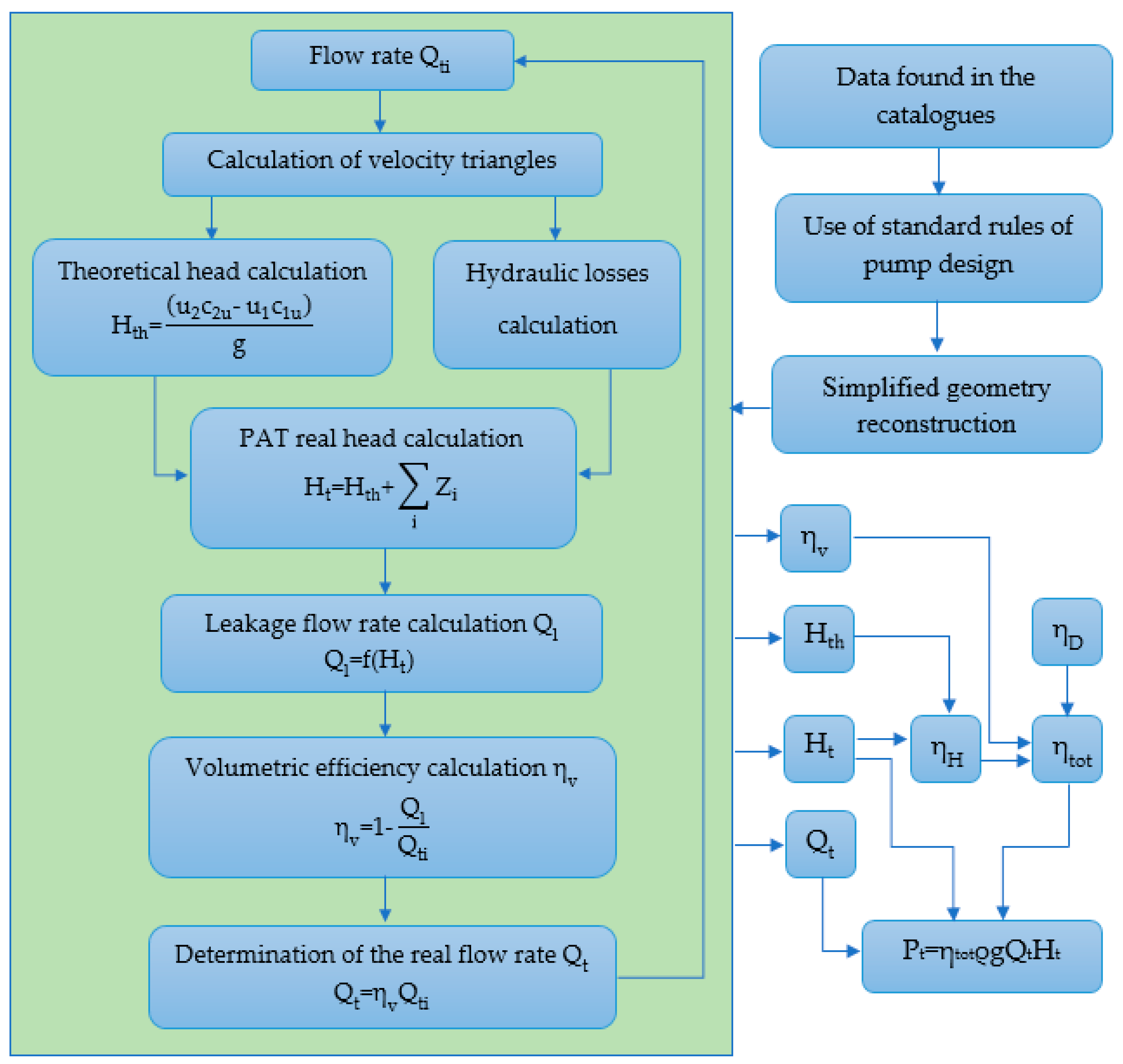
4.2. 1D Models That Recreate the Geometry of the Machine

Several authors such as Barbarelli et al. [27] and Manservigi et al. [28] proposed one-dimensional models able to recreate the unspecified geometry of the machine, starting from data that can be found in the catalogues provided by pump manufacturers. In a such way, it is possible to obtain a better prediction accuracy in comparison with empirical models, without restricting the scope of the method.

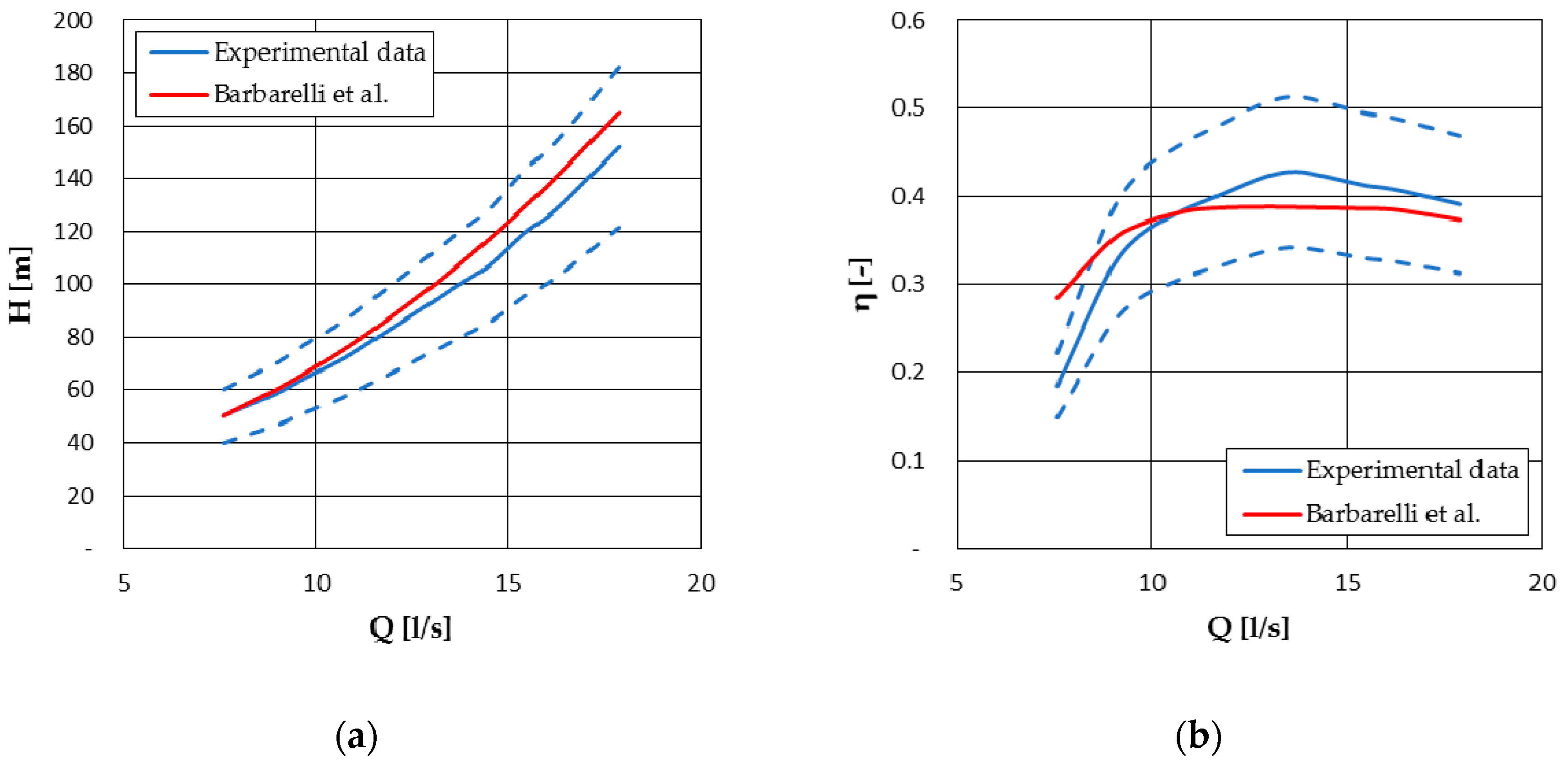
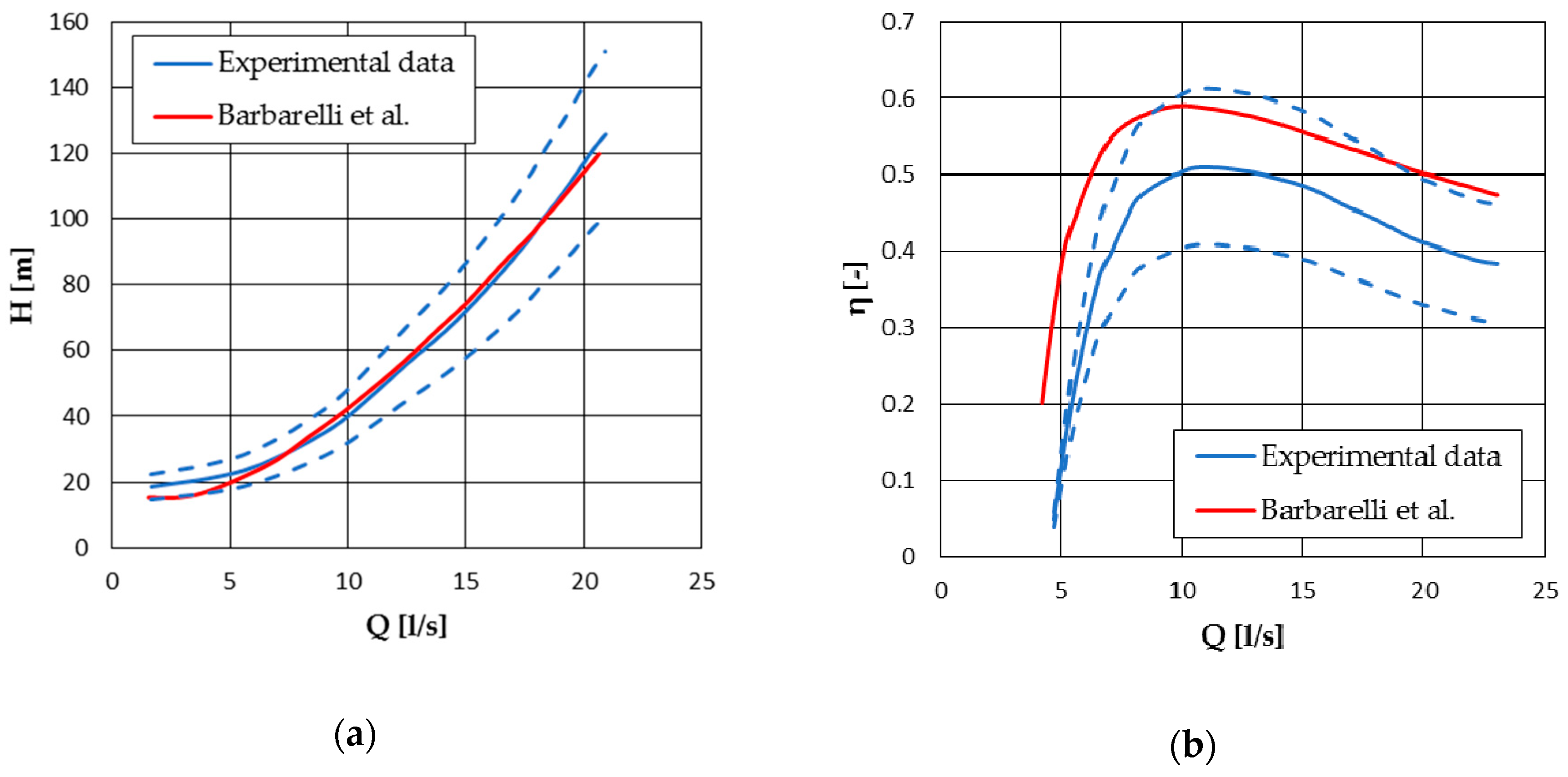
4.2.1. Barbarelli et al. Model

The first step of the model proposed by Barbarelli et al. [27] includes defining a simplified geometry, starting from the following data, which can be found in the manufacturer’s catalogues:
  • Pump head at BEP
  • Pump flow rate at BEP
  • Maximum power
  • Head at zero flow
  • Impeller diameter
  • Size of the pump
Geometry is reconstructed using standard rules usually followed by pump manufacturers. The second part of the models consists of an iterative procedure necessary to identify the value of the volumetric efficiency [27]. In fact, the leakage flow rate is unknown and is expressed by the authors as a function of PAT head, that needs to be obtained. This procedure involves the calculation of hydraulic losses, divided into friction losses Zf and dynamic losses Zd expressed by the authors by means of Equations (15) and (16) [27].
Z f   =   λ c 2 2 g ( l D h )
Z d   =   ξ c 2 2 g
Compared to the study previously proposed by Amelio and Barbarelli [29], the main difference is the addition of a loss related to low flow rates and calculated with Equation (17) [27].
Z lowflow   =   K ( Q t Q BEPt ) 2
The parameter K, present in the equation above, can be estimated by means of the Equation (18), derived by Barbarelli et al. [27] from a statistical analysis of data acquired at a test rig.
K   =   1 53.67 + 0.0077   n st 3.44
Starting from a guessed value of the flow rate Qti, the velocity triangles can be obtained in the inlet and outlet section of the impeller, so that PAT theoretical head can be calculated. Subsequently, hydraulic losses are calculated to obtain the real head of the PAT. After that, it is possible to determine the leakage flow rate, considered by Barbarelli et al. [27] as a function of the real head of the PAT. The authors proposed the calculation of the volumetric efficiency using Equation (19) [27,29]
η v   =   1 Q l Q ti   =   Q t Q ti
By means of this iterative procedure the head curve is obtained, but Barbarelli et al. [27] also proposed the calculation of the other performance curves. To obtain the efficiency curve, in parallel to volumetric efficiency, hydraulic efficiency ηH and disc efficiency ηD are needed, as reported in the following equation:
η tot   =   η v η H η D
Finally, Equation (21) can be used to calculate the power curve.
P t   =   η tot ρ gQ t H t
Figure 1 summarizes the entire procedure that allows the user to obtain the characteristic curves of a PAT, starting from data that can be found in manufacturer’s catalogues.
It is worth pointing out that the model proposed by Barbarelli et al. [27] can work in three different modes, depending on the user’s need:
  • Design mode
  • Known geometry mode
  • Mixed mode
In the first case, the user only knows geometric parameters that can be found in manufacturer’s catalogues and can be a valid tool for a designer who wants to use a PAT in a given hydropower site. Vice versa, the second option requires detailed geometrical information of the machine and can be easily used by manufacturers to better understand the behavior of their pumps running in reverse mode. The last of the three listed, mixed mode, can be used if there is a partial knowledge of geometrical parameters, beyond the ones present in manufacturer’s catalogues.

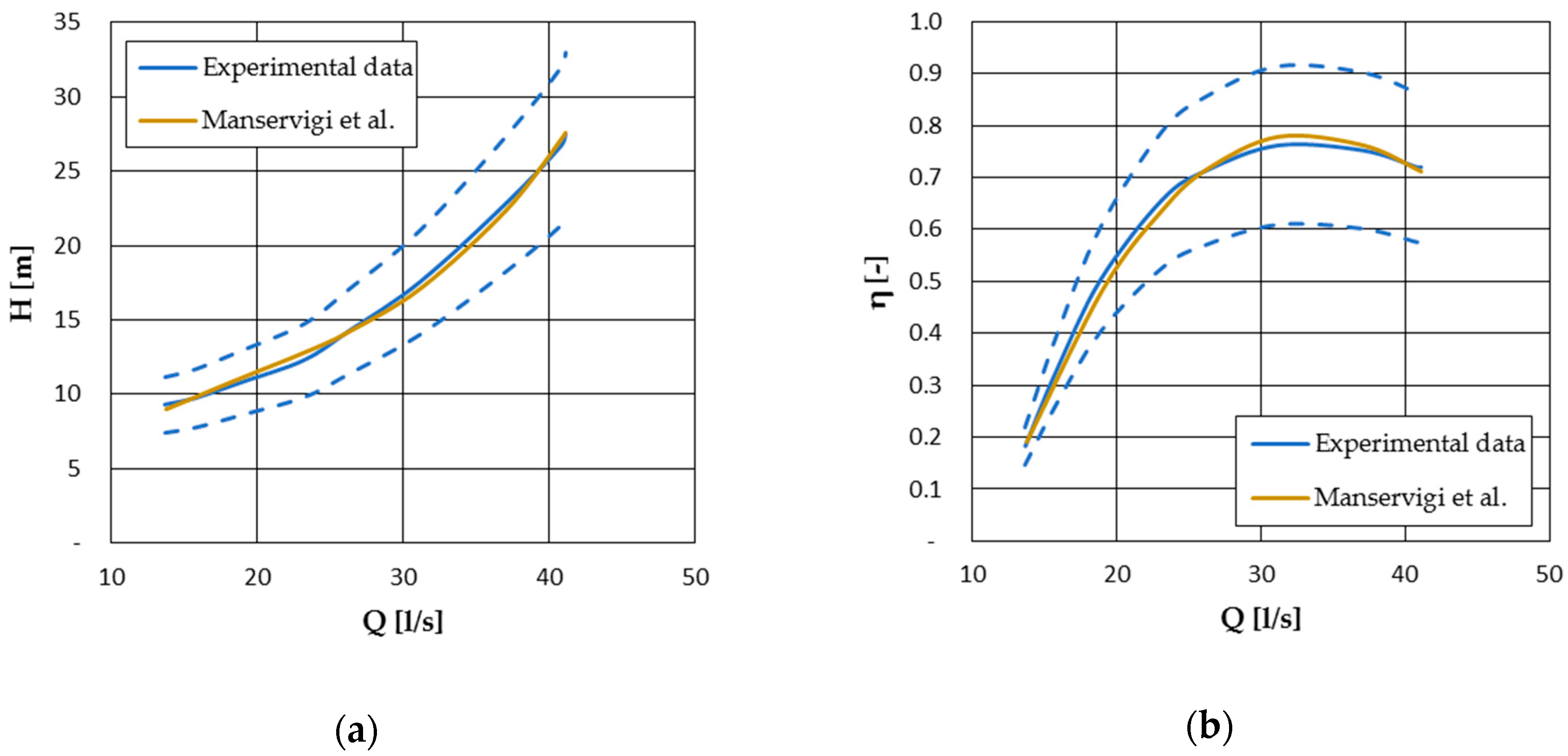
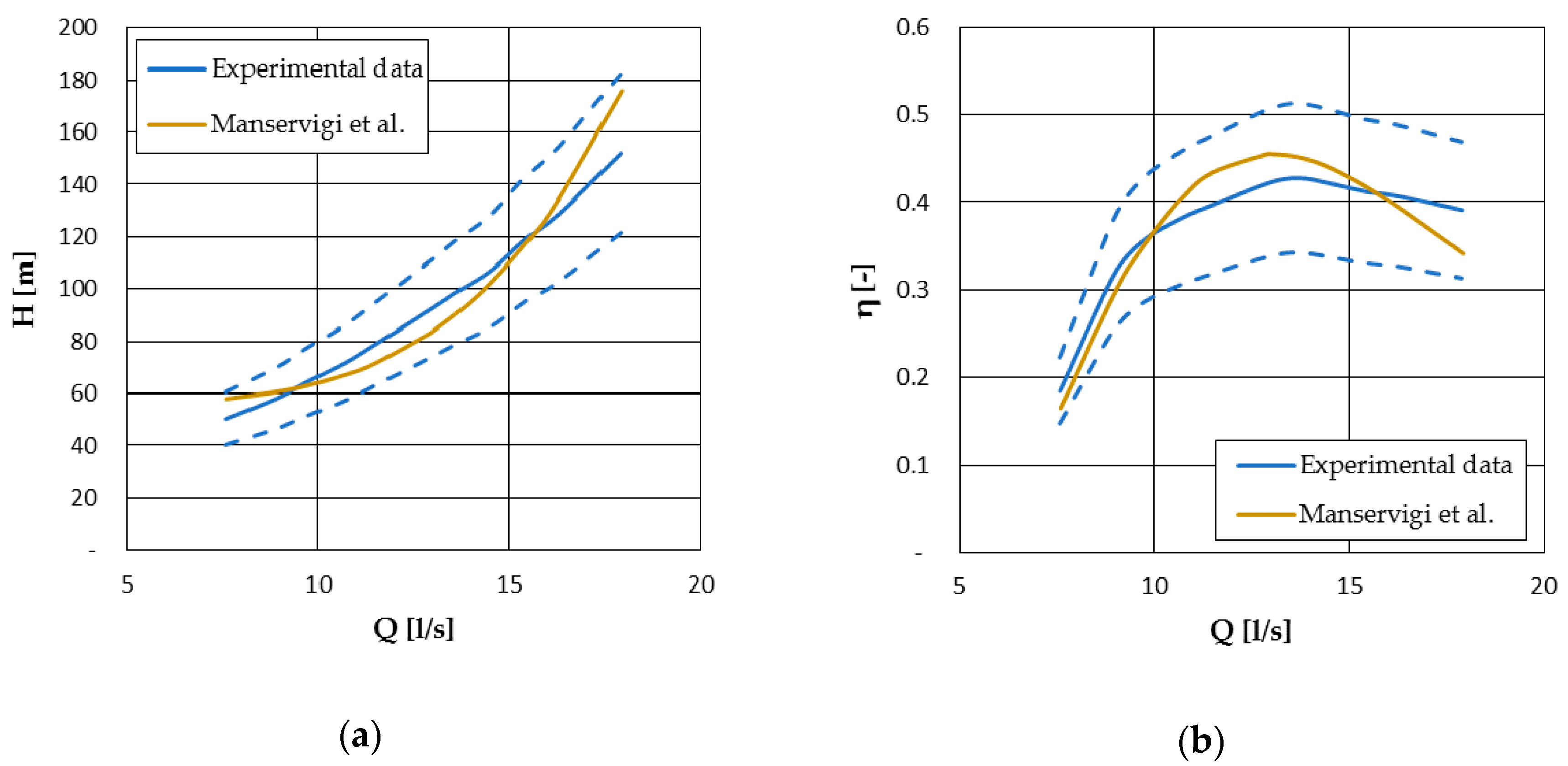
4.2.2. Manservigi et al. Model

Manservigi et al. [28] proposed a model capable of calculating the characteristic curves of a PAT, starting from the ones related to the pump. This model is based on an iterative procedure with the aim of optimizing the value of 24 parameters, 14 of them related to the pump, the other 10 related to the PAT. These parameters refer not only to the geometry of the machine, but also to hydraulic and power losses and some of them relate the BEP of the PAT to the pump corresponding one.
Through the use of these 24 parameters, it is possible to calculate the performance curves of a machine in direct and reverse running mode. In particular, regarding the PAT physical modelling, proposed by Manservigi et al. [28], starting from the theoretical head, the real head of the PAT is known adding the hydraulic losses, as expressed by Equation (22).
H t   =   H th + i Z i
The power curve can be obtained considering hydraulic efficiency ηH, flow rate Qt, leakage flow rate Ql and power losses L using the following equation:
P t   =   ρ gH t η H ( Q t Q l ) i L i
The efficiency curve can be easily obtained by means of Equation (24).
η t   =   P t ρ gH t Q t
Actually, the authors refer to the following dimensionless parameters for the performance curves [28]:
  • Head coefficient ψ
  • Power coefficient π
  • Efficiency η
where ψ and π are defined in Equations (25) and (26) [28].
ψ   =   gH n 2 D 2
π   =   P ρ n 3 D 5
Pump performance curve obtained using the model are compared to the ones provided by pump manufacturers through the parameter Root Mean Square Relative Error (RMSE), defined as:
RMSE   =   1 N i = 1 N ( X exp i X s i X exp i ) 2
where Xexp and Xs refer to experimental and simulated values, respectively, and N is the number of values available. The optimization procedure minimizes the sum of RMSEs for the performance curves to find the optimal values of the 24 parameters, thus, to reconstruct pump and PAT performance curves. Moreover, the optimization procedure can regard direct and reverse running mode separately or simultaneously [28].

4.3. 1D Models That Use a Known Geometry

One-dimensional models based on a known geometry are developed with the aim of obtaining more accurate predictions related to methods that recreate a simplified geometry of the machine. Stefanizzi et al. [30] proposed a method belonging to this typology, that can be, as the authors suggest, a reliable tool for pump manufacturers that want to better know the reverse running behavior of their machines. In fact, the complexity of this method is too high to consider it intended for a designer of a small hydropower plant.
The first step of this methodology consists of collecting detailed geometrical information of the machine, and then establish the flow rate Qt and the rotational speed nt related to the PAT. This is required to obtain the velocity triangles, in particular the circumferential components of the absolute velocities c2u and c1u. Thanks to the previous step, it is possible to calculate the theoretical head using Equation (28) and, subsequently, to obtain the real head of the PAT, taking into account hydraulic losses in the volute Zv and in the impeller (runner) Zr, using Equation (29).
H th   =   ( u 2 c 2 u   u 1 c 1 u ) g
H t   =   σ PAT H th + Z v + Z r
Moreover, Stefanizzi et al. [30] also considered a correlation for a slip factor σPAT, obtained by Capurso et al. [31] by means of a CFD analysis and reported in Equation (30).
σ PAT   =   0.2365 ( Q Q BEPp ) 2 0.5537 ( Q Q BEPp ) + 1.2846

4.4. 3D-CFD Models

Three-dimensional models based on computational fluid dynamics concerning PATs are being used in different ways, as discussed in the following.
Frosina et al. [32] developed a model to analyze the behavior of three commercial pumps with different specific speeds running in direct and reverse mode. Starting with the real geometry, the authors extracted the fluid volume and then meshed it using the software PumpLinx®, which is also able to numerically solve the Navier–Stockes equations. Moreover, Frosina et al. [32] considered a k-ε turbulence model that led to good accuracy and computational efficiency. The model was validated in two steps, the first one was related to the pump characteristic curves which were effectively compared to the ones provided by pump manufacturer. The second part of the validation process compared the simulated PAT curves in terms of pressure with experimental data. Thus, having validated the entire model Frosina et al. [32] finally obtained PAT performance curves.
Perez–Sanchez et al. [33] developed a 3D-CFD model to analyze the behavior of a reverse-running pump used to reduce pressure in a WDN. First, the authors created a 3D geometrical model by means of a CAD software. The authors discretized the governing equations using the finite volume method and considered for the turbulence the k-ε model with wall functions, based on the following additional equations:
ρ k t + x i ( ρ u i k )   =   x i ( ( μ + μ t o k ) k x i ) + s k
ρ ε t + x i ( ρ u i ε )   =   x i ( ( μ + μ t o ε ) ε x i ) + s ε
Furthermore, Perez–Sanchez et al. [31] validated the model comparing its results to experimental data acquired using of a purpose-made test rig obtaining good agreement.
Moreover, several authors like Yang et al. [23], Rossi et al. [34] and Stefanizzi et al. [30] used computational fluid dynamics for validating models of the typologies previously described.
Finally, Li [35] used computational fluid dynamics to analyze the behavior of PAT characteristic curves considering water and four different types of viscous oils, thus considering fluids with different kinematic viscosity. This study is relevant because, in some PAT applications in industrial processes, the working fluid can be different from water.

5. Applicability of the Various Methods

The aim of the study presented in this paper is mainly to appreciate advantages and disadvantages of the various models to assess their applicability for analysis.
Some basic models can be immediately applied for selecting the PAT to be used, starting from the hydraulic resource information. This can be an important factor, in parallel to the method accuracy. Other basic models, which correlate the conversion factor to pump parameters, should be applied in a more complex way.
The operating point can be identified by intersecting the site characteristic curve with the PAT characteristic curve, thus appropriate models are needed. Methods that can predict the characteristic curves of a PAT are not always simple to apply. In fact, they can require the knowledge of detailed geometrical information as well as involve iterative procedures. Usually, an increase in complexity corresponds to a decrease in the prediction error, but, for a small hydropower plant designer, an appropriate balance between simplicity and accuracy is desirable.
In this section the behavior of basic models is described, as well as the one of more complex methods able to calculate PAT characteristic curves.

5.1. Basic Models

Basic models, described in Section 3, are considered in this study as a valid tool for selecting the PAT to be used in a small hydropower plant. These methods correlate the two conversion factors CQ and CH to different parameters, but the most advantageous for selecting a machine, starting from the site parameters, are the ones that express CQ and CH as a function of PAT specific speed.
In fact, by knowing head Hsite = HBEPt and flow rate Qsite = QBEPt related to the hydraulic resource, as well as the PAT rotational speed, it is possible to calculate the required PAT specific speed nst. Using the conversion factors is possible to calculate the pump corresponding parameters (QBEPp and HBEPp), thus the machine is selected from manufacturer’s catalogue. From this point of view, it is easy to use the models proposed by Algieri et al. [9], Barbarelli et al. [11], Derakhshan and Nourbakhsh [19], Grover [20], Hergt [20] and Stefanizzi [22].
Other basic models cannot be applied in a direct way. For example, the model proposed by Alattore–Frenk [17] correlates the two conversion factors to pump efficiency at BEP ηBEPp and it should be applied through trial and error. In fact, starting from catalogue information, pump flow rate QBEPp, head HBEPp and efficiency ηBEPp at BEP are known, thus, it is possible to calculate CQ and CH. Subsequently, PAT flow rate QBEPt and head HBEPt at BEP can be obtained. Several attempts may be needed in such a way that these PAT parameters match site flow rate and head.
Thereby, the statistical approach that correlates the conversion factors to the specific speed of the PAT seems to be the best solution. As an example, the curves proposed by Barbarelli et al. [11] are reported in Figure 2.
It is likewise important to evaluate basic models’ accuracy and, for this purpose, it is possible to use the Williams criterion [20]. It is therefore necessary, as well as difficult, to find a data set wide enough to compare basic models in a proper way.

5.2. Models That Predict the Characteristic Curves of a PAT

The models able to predict the characteristic curves of a PAT are necessary to identify the operating point of a PAT in a hydropower plant and to estimate the producible energy. As described in Section 4, different typologies of models were developed by several researchers and every kind of method is characterized by advantages and drawbacks. The aim of this section is to analyze the behavior of the models previously described trying to explain how and why they can be useful.
First, it needs to be specified that, in the following, some results are presented for empirical models and one-dimensional models that recreate the machine geometry. These results were obtained by applying the models to the pumps tested by Barbarelli et al. [11] in direct and reverse mode and listed in the following: KSB 40-335, KSB 40-315, KSB 40-250, KSB 40-220, Av 65-250, Av 80-250, KSB 50-160, KSB 80-200, KSB 80-220, KSB 100-200 and KSB 125-200. All KSB pumps belong to the Etanorm series and the naming convention consists of two numbers; the first one is the nominal discharge nozzle diameter [mm] and the second one is the nominal impeller diameter [mm]. Moreover, in every following figure, a 20% wide error band is reported, so that is possible to better evaluate the model accuracy.
Among the empirical models, the one proposed by Derakhshan and Nourbakhsh [19] is now considered. In particular, this empirical method is composed by a first part able to correlate the BEP of a pump with the PAT corresponding one and a second part that allows to obtain the characteristic curves of a PAT. These two parts were separately discussed in the Section 3 and Section 4.1.1, but now are considered as a whole procedure.
As easily deductible from Figure 3, in some cases the model proposed by Derakhshan and Nourbakhsh [19] led to good accuracy as for the PAT 80–200, with both head and efficiency curves contained in the 20% wide error bands.
Things are completely different in Figure 4 related to the PAT 40–335 where both head and efficiency curves are unable to follow the trend of experimental data. This can be explained considering the pump specific speed of the machine, which is equal to 9.08. In fact, even if Derakhshan and Nourbakhsh [19] consider their method valid for pumps with a specific speed less than 60, the machines used in the setup phase of the model were in the range 14–56, therefore, model accuracy in identifying the BEP in reverse-running mode can be compromised outside this interval. Moreover, it is worth observing that PAT 40–335 is an atypical machine with a flow field characterized by high deflections. Figure 5 refers to the same PAT, but calculations were made considering the real BEP of the PAT and the predicted head and efficiency curves present a noticeable improvement.
Thus, the model developed by Derakhshan and Nourbakhsh [19] has its strength in the simplicity but this study highlighted that the method is particularly sensitive to identification of the BEP of the PAT and predictions can be prejudiced. Moreover, the range of application is limited to pumps with specific speed less than 60.
The one-dimensional model developed by Barbarelli et al. [27] in most cases led to good accuracy, as reported in Figure 6 related to the PAT 40–335. Head curve is contained in the 20% wide error band, as well as efficiency curve except for a low flow rate zone.
For the PAT 40–250 (Figure 7) head curve was recreated with high accuracy and efficiency curve is able to follow the trend of experimental data even if is slightly shifted upwards.
This analysis demonstrates that the method proposed by Barbarelli et al. [27] is robust and accurate and even if the model is not able to perfectly recreate the experimental curves, the error is however limited. Moreover, this model is characterized by a wide range of application. It is also important to highlight the detailed hydraulic losses modelling utilized by the authors in developing this method (hydraulic losses calculated in each flow section: Inlet, volute, diffuser, impeller and discharge), even if predictions could be improved by a better geometry reconstruction.
The model proposed by Manservigi et al. [28] showed good accuracy in most cases, for example in Figure 8 head and efficiency curves for the PAT 80–200 are shown.
In other cases, as for the PAT 40–335, both head and efficiency curves are not in perfect agreement with the trend of experimental data but are however contained in the 20% wide error bands (Figure 9).
The method proposed by Manservigi et al. [28] proved to be robust and accurate and the most noteworthy part of the model is the iterative procedure able to optimize the value of 24 parameters that allows, among other things, to reconstruct the machine geometry. This procedure also provides the coefficients for hydraulic losses that could be calculated in a more consistent way to improve the model reliability.
One-dimensional models based on a known geometry, as the one proposed by Stefanizzi et al. [30], can be a reliable tool for pump manufacturers who want to analyze the reverse running behavior of their machines. This kind of model, due to the high complexity, is not intended to be used by small hydropower plant designers. In fact, detailed geometrical information is not easy to obtain and the machine should be disassembled. Therefore, despite the high accuracy reported by the authors, this type of model suffers from the high level of resources required.
3D-computational fluid dynamics models can be effectively used to validate method of other typologies and to analyze the flow field in a PAT, as well as the influence of parameters like the kinematic viscosity [34,35]. Furthermore, CFD can be helpful in the setup phase of some models obtaining correlations to be implemented, for example for the calculation of the slip factor [31]. Due to the complexity and the computational expense, these methods are prohibitive for a small hydropower plant designer.

6. Discussion

PATs can be effectively used for exploiting small hydraulic resources, but it is important to have information on their performances to properly select the machine to be used and to obtain the operating point. To this end, basic models and methods able to predict PAT characteristic curves are needed.
As previously stated, basic models which correlate the conversion factors CQ and CH to PAT specific speed, can be immediately used for the selection of the machine. This aspect is underlined in Table 2, in which the possibility to apply the model starting from site data is remarked with the symbol ✘. Moreover, Table 2 highlights the output of basic models as well as the kind of analysis from which the correlations derive, namely theoretical considerations or experimental data.
To identify the operating point of a PAT it is necessary to use methods able to predict its characteristic curves. This study highlighted the possibility of a model that predicts PAT characteristic curves to be based on experimental data, theoretical considerations or CFD. This aspect, in parallel to input and output of the methods reviewed, is reported in Table 3, where the symbol ✘ means, once again, the presence of a factor for the considered model.
From the analysis presented on the previous section, it is easy to observe that methods able to predict PAT performance curves starting from data found in pump catalogues are the ones useful for a small hydropower plant designer. Thus, the focus of this discussion regards empirical models and 1D models that recreate the PAT geometry.
These models can obtain good results for a machine, but cannot be properly applied to other PATs. This is a common problem in PAT performance predicting models, but it is possible to consider the advantages of the various methods and to unite them obtaining a more reliable strategy.
Empirical models, as the one proposed by Derakhshan and Nourbakhsh [19], are simple to apply, but they are seldom robust and are valid in a limited range of the specific speed of the machine.
The one-dimensional model developed by Barbarelli at al. [27] presents a detailed modelling of dynamic losses and a wide range of application. Its main drawback is the improvable geometry reconstruction.
The advantage of the model proposed by Manservigi et al. [28] is the geometry reconstruction by means of an optimization procedure but the result is dependent on hydraulic losses modelling, considered by the authors in a simplified way.
Both the models proposed by Barbarelli et al. [27] and Manservigi et al. [28] behave well, but the results shown in the previous section are related to machines used in their set up phase. Thus, it should be necessary to apply the models to a greater number of different machines. In fact, despite the good results, both the methods cited above could introduce calculation errors on model parameters that compensate each other and lead to a global error near to zero. The increase in the number of cases examined gives the possibility to highlight and correct this criticality.
Furthermore, future developments may involve disassembling these methods to consider the best parts of each, with the aim of combining them and creating a new tool, more reliable but not more complex. In this regard, it seems possible to combine the optimization procedure for the geometry reconstruction proposed by Manservigi et al. [28] with the detailed model of hydraulic losses proposed by Barbarelli et al. [27].
Finally, it is noted that no general evaluation criterion is documented in the literature for the various methods capable of predicting the characteristic curves of a PAT, as it can be done for basic models using the Williams criterion. To this end, the authors of this article have the idea of creating a comparison index based on:
  • Prediction error
  • Simplicity of application
  • Number of parameters involved

7. Conclusions

In this paper a review of methods used for selecting PATs and predicting their characteristic curves has been presented. The models developed by several researchers have been described and, after that, advantages and drawbacks have been analyzed. The aim of the study was to provide information useful for a designer of a small hydropower plant, who wants to use a PAT, in selecting the proper machine and obtaining the operating point.
Basic models, able to correlate pump BEP to the PAT corresponding one, can be used for a preliminary selection of the machine. In particular, models which calculate the conversion factors CQ and CH as a function of the PAT specific speed seem to be the most suitable in this regard.
Obtaining the PAT operating point is crucial in the estimation of the produced energy, thus models able to predict PAT performance curves are required. Various approaches have been used to this purpose, namely empirical model, 1D models (with known geometry or able to reconstruct it), 2D models and 3D-CFD models. 2D models are considered as a valid tool to calculate correlations for the slip factor of turbomachinery and were not analyzed in this study.
1D models that require a known geometry and 3D-CFD models were considered prohibitive for a small hydropower plant designer due to the complexity and computational expense. The methods able to predict PAT performance curves starting from data found in pump catalogues are the empirical models and 1D models able to reconstruct the machine geometry. Empirical models are simple but usually not robust, thus the study focused on the models proposed by Barbarelli et al. [27] and Manservigi et al. [28] as a sample of one-dimensional models that reconstruct PAT geometry. The study highlighted the possibility to disassemble these two models and to merge their best parts with the aim to obtain a more reliable strategy.

Author Contributions

Conceptualization, methodology, software, writing—review and editing, S.B. Pumps As Turbines formal analysis, data curation, writing—original draft preparation, review and editing, D.S.; supervision, project administration, writing—review and editing, M.A. All authors have read and agreed to the published version of the manuscript.

Funding

This research received no external funding.

Conflicts of Interest

The authors declare no conflict of interest.

Nomenclature

BEP Best Efficiency Point
c Absolute velocity
c 1 u Circumferential component of absolute velocity in PAT impeller outlet section
c 2 u Circumferential component of absolute velocity in PAT impeller inlet section
CFD Computational Fluid Dynamics
C H Head conversion factor
C Q Flow rate conversion factor
D Impeller diameter
D h Hydraulic diameter
g Gravitational acceleration
h Ratio between PAT head and PAT head at BEP
H Head
H BEP Head at BEP
H BEPp Pump head at BEP
H BEPt PAT head at BEP
H site Site head
H t PAT head
H th Theoretical head
i Index of the summation
k Turbulent kinetic energy
K Parameter necessary at Zlowflow calculation
l Length
L Power loss
n Rotational speed
N Number of data
n p Pump rotational speed
n st PAT specific speed
n t PAT rotational speed
p Ratio between PAT power and PAT power at BEP
P Power
PAT Pump As Turbine
P BEP Power at BEP
P BEPt PAT power at BEP
PHES Pumped-Hydro Energy Storage
PRV Pressure Reducing Valve
P t PAT power
q Ratio between PAT flow rate and PAT flow rate at BEP
Q Flow rate
Q BEP Flow rate at BEP
Q BEPp Pump flow rate at BEP
Q BEPt PAT flow rate at BEP
Q l Leakage flow rate
Q site Site flow rate
Q t PAT flow rate
Q ti PAT flow rate – initial value at the i-th iteration
RSME Root Mean Square Relative Error
S k ,   S ε Source term
u 1 Tangential velocity in PAT impeller outlet section
u 2 Tangential velocity in PAT impeller inlet section
u i Fluid velocity in the xi direction
WDN Water Distribution Network
x i Generic axis direction
X exp Experimental value of a quantity
X s Simulated value of a quantity
Z Hydraulic loss
Z d Dynamic loss
Z f Friction loss
Z lowflow Hydraulic loss at low flow rate
Z r Runner hydraulic loss
Z v Volute hydraulic loss
α , βDimensionless specific speed
α p , β p Dimensionless pump specific speed
α t , β t Dimensionless PAT specific speed
γ Dimensionless parameter necessary to calculate CH
ε Rate of dissipation of turbulent kinetic energy
η Efficiency
η BEP Efficiency at BEP
η D Disc efficiency
η H Hydraulic efficiency
η HBEP Hydraulic efficiency at BEP (pump mode)
η t PAT efficiency
η tot PAT total efficiency
η v Volumetric efficiency
η BEPp Pump efficiency at BEP
η BEPt PAT efficiency at BEP
η p Pump efficiency
λFriction coefficient
μDynamic viscosity
μtTurbulent viscosity
ξDynamic loss coefficient
π Power coefficient
ρ Density
σ k ,   σ ε Adjustable constant
σ PAT PAT slip factor
ψ Head coefficient

References

  1. Chapallaz, J.M.; Eichenberger, P.; Fischer, G. Manual on Pumps Used as Turbines; Vieweg: Braunschweig, Germany, 1992. [Google Scholar]
  2. Patelis, M.; Kanakoudis, V.; Gonelas, K. Pressure management and energy recovery capabilities using PATs. Procedia Eng. 2016, 162, 503–510. [Google Scholar] [CrossRef]
  3. Meirelles Lima, G.; Luvizotto, E., Jr.; Brentan, B.M. Selection of Pumps as Turbines Substituting Pressure Reducing Valves. Procedia Eng. 2017, 186, 676–683. [Google Scholar] [CrossRef]
  4. Alberizzi, J.C.; Renzi, M.; Nigro, A.; Rossi, M. Study of a Pump-as-Turbine (PaT) speed control for a Water Distribution Network (WDN) in South-Tyrol subjected to high variable water flow rates. Energy Procedia 2018, 148, 226–233. [Google Scholar] [CrossRef]
  5. Venturini, M.; Alvisi, S.; Simani, S.; Manservigi, L. Energy Production by Means of Pumps as Turbine in Water Distribution Networks. Energies 2017, 10, 1666. [Google Scholar] [CrossRef] [Green Version]
  6. Rossi, M.; Nigro, A.; Pisaturo, G.R.; Renzi, M. Technical and economic analysis of Pump-as-Turbine (PaT) used in Italian Water Distribution Network (WDN) for electrical energy production. Energy Procedia 2019, 158, 117–122. [Google Scholar] [CrossRef]
  7. Barbarelli, S.; Amelio, M.; Florio, G.; Scornaienchi, N.M. Procedure Selecting Pumps Running as Turbines in Micro Hydro Plants. Energy Procedia 2017, 126, 549–556. [Google Scholar] [CrossRef]
  8. Barbarelli, S.; Amelio, M.; Florio, G. Using a statistical-numerical procedure for the selection of pumps running as turbines to be applied in water pipelines: Study cases. J. Sustain. Dev. Energy Water Environ. Syst. 2018, 6, 323–340. [Google Scholar] [CrossRef] [Green Version]
  9. Algieri, A.; Zema, D.A.; Nicotra, A.; Zimbone, S.M. Potential energy exploitation in collective irrigation systems using pumps as turbines: A case study in Calabria (Southern Italy). J. Clean. Prod. 2020, 257, 120538. [Google Scholar] [CrossRef]
  10. Renzi, M.; Rudolf, P.; Stefan, D.; Nigro, A.; Rossi, M. Energy recovery in oil refineries through the installation of axial Pumps-as-Turbines (PATs) in a wastewater sewer: A case study. Energy Procedia 2019, 158, 135–141. [Google Scholar] [CrossRef]
  11. Barbarelli, S.; Amelio, M.; Florio, G. Experimental activity at test rig validating correlations to select pumps running as turbines in microhydro plants. Energy Convers. Manag. 2017, 149, 781–797. [Google Scholar] [CrossRef]
  12. Sivakumar, N.; Das, D.; Padhy, N.P. Economic analysis of Indian pumped storage schemes. Energy Convers. Manag. 2014, 88, 168–176. [Google Scholar] [CrossRef]
  13. Scheliecher, W.C.; Oztekin, A. Hydraulic design and optimisation of a modular pump-turbine runner. Energy Convers. Manag. 2015, 93, 388–398. [Google Scholar] [CrossRef] [Green Version]
  14. Williams, A.A.; Simpson, R. Pico hydro—Reducing technical risks for rural electrification. Renew. Energy 2009, 34, 1986–1991. [Google Scholar] [CrossRef]
  15. Arriaga, M. Pump as turbine—A pico-hydro alternative in Lao People’s Democratic Republic. Renew. Energy 2010, 35, 1109–1115. [Google Scholar] [CrossRef]
  16. Motwani, K.H.; Jain, S.V.; Patel, R.N. Cost analysis of pump as turbine for pico hydropower plants—A case study. Procedia Eng. 2013, 51, 721–726. [Google Scholar] [CrossRef] [Green Version]
  17. Alatorre-Frenk, C.; Thomas, T.H. The Pumps-As-Turbines (PATs) Approach to Small Hydropower; Word Congress on Renewable Energy: Reading, UK, 1990. [Google Scholar]
  18. Childs, S.M. Convert Pumps to Turbines and Recover HP. Hydrocarb. Process. Pet. Refin. 1962, 41, 173–174. [Google Scholar]
  19. Derakhshan, S.; Nourbakhsh, A. Experimental study of characteristic curves of centrifugal pumps working as turbines in different specific speed. Exp. Therm. Fluid Sci. 2008, 32, 800–807. [Google Scholar] [CrossRef]
  20. Williams, A.A. The turbine performance of centrifugal pumps: A comparison of prediction methods. Proc. Inst. Mech. Eng. 1994, 208, 59–66. [Google Scholar] [CrossRef]
  21. Hancock, J.W. Centrifugal Pump or Water Turbine. Pump Line News 1963, 6, 25–27. [Google Scholar]
  22. Stefanizzi, M. Theoretical and Expertimental Analysis of Pumps as Turbines. Ph.D. Thesis, Politecnico di Bari, Bari, Italy, 2018. [Google Scholar]
  23. Yang, S.S.; Derakhshan, S.; Kong, F.Y. Theoretical, numerical and experimental prediction of pump as turbine preformance. Renew. Energy 2012, 48, 507–513. [Google Scholar] [CrossRef]
  24. Visser, F.C.; Brouwers, J.J.H.; Badie, R. Theoretical analysis of inertially irrootational and solenoidal flow in two-dimensional radial-flow pump and turbine impellers with equiangular blades. J. Fluid Mech. 1994, 269, 107–141. [Google Scholar] [CrossRef] [Green Version]
  25. Paeng, K.S.; Chung, M.K. A new slip factor for centrifugal impellers. Proc. Inst. Mech. Eng. 2001, 215, 645–649. [Google Scholar] [CrossRef]
  26. Rossi, M.; Renzi, M. Analytical Prediction Models for Evaluating Pump-As-Turbines (PATs) Performance. Energy Procedia 2017, 118, 238–242. [Google Scholar] [CrossRef]
  27. Barbarelli, S.; Amelio, M.; Florio, G. Predictive model estimating the performances of centrifugal pumps used as turbines. Energy 2016, 107, 103–121. [Google Scholar] [CrossRef]
  28. Manservigi, L.; Venturini, M.; Losi, E. Application of a physics-based model to predict the performance curves of pumps as turbines. AIP Conf. Proc. 2019, 2191, 020106. [Google Scholar]
  29. Amelio, M.; Barbarelli, S. A one-dimensional numerical model for calculating the efficiency of pumps as turbines for implementation in micro-hydro power plants. In Proceedings of the ESDA: 7th Biennal ASME Conference Engineering Systems Design and Analysis, Manchester, UK, 19–22 July 2004. [Google Scholar]
  30. Stefanizzi, M.; Capurso, T.; Torresi, M.; Pascazio, G.; Ranaldo, S.; Camporeale, S.M.; Fortunato, B.; Monteriso, R. Development of a 1-D Performance Prediction Model for Pumps as Turbines. In Proceedings of the 3rd EWaS International Conference, Lefkada, Greece, 27–30 June 2018. [Google Scholar]
  31. Capurso, T.; Stefanizzi, M.; Pascazio, G.; Ranaldo, S.; Camporeale, S.M.; Fortunato, B.; Torresi, M. Slip Factor Correction in 1-D Performance Prediction Model for PATs. Water 2019, 11, 565. [Google Scholar] [CrossRef] [Green Version]
  32. Frosina, E.; Buono, D.; Senatore, A. A Performance Prediction Method for Pumps as Turbines (PAT) Using a Computational Fluid Dynamics (CFD) Modeling Approach. Energies 2017, 10, 103. [Google Scholar] [CrossRef] [Green Version]
  33. Perez-Sanchez, M.; Simao, M.; Lopez-Jimenez, P.A.; Ramos, H.M. CFD Analyses and Experiments in a PAT Modeling: Pressure Variation and System Efficiency. Fluids 2017, 2, 51. [Google Scholar] [CrossRef] [Green Version]
  34. Rossi, M.; Nigro, A.; Renzi, M. Experimental and numerical assessment of a methodology for performance prediction Pumps-as-Turbines (PATs) operating in off-design conditions. Appl. Energy 2019, 248, 555–566. [Google Scholar] [CrossRef]
  35. Li, W.G. Effects of viscosity on turbine mode performance and flow of a low specific speed centrifugal pump. Appl. Math. Model. 2016, 40, 904–926. [Google Scholar] [CrossRef]
Figure 1. Flow diagram of the model proposed by Barbarelli et al. [27].
Energies 13 06341 g001
Figure 2. Conversion factors as a function of Pumps As Turbine (PAT) specific speed, according to Barbarelli et al. [11] (a) flow rate conversion factor and (b) head conversion factor.
Energies 13 06341 g002
Figure 3. Results of the model proposed by Derakhshan and Nourbaksh [19] for the PAT 80–200 compared to experimental data (a) head curves and (b) efficiency curves.
Energies 13 06341 g003
Figure 4. Results of the model proposed by Derakhshan and Nourbaksh [19] for the PAT 40–335 compared to experimental data (a) head curves and (b) efficiency curves.
Energies 13 06341 g004
Figure 5. Results of the model proposed by Derakhshan and Nourbaksh [19] for the PAT 40–335 compared to experimental data, using the real Best Efficiency Point (BEP) of the PAT (a) head curves and (b) efficiency curves.
Energies 13 06341 g005
Figure 6. Results of the model proposed by Barbarelli et al. [27] for the PAT 40–335 compared to experimental data (a) head curves and (b) efficiency curves.
Energies 13 06341 g006
Figure 7. Results of the model proposed by Barbarelli et al. [27] for the PAT 40–250 compared to experimental data (a) head curves and (b) efficiency curves.
Energies 13 06341 g007
Figure 8. Results of the model proposed by Manservigi et al. [28] for the PAT 80–200 compared to experimental data (a) head curves and (b) efficiency curves.
Energies 13 06341 g008
Figure 9. Results of the model proposed by Manservigi et al. [28] for the PAT 40–335 compared to experimental data (a) head curves and (b) efficiency curves.
Energies 13 06341 g009
Table 1. Basic models correlations for the calculation of the conversion factors [9,11,17,18,20,21,22,23].
Model C Q C H
Alatorre–Frenk 0.85   η BEPp 5 + 0.385 2   η BEPp 9.5 + 0.205 1 0.85   η BEPp 5 + 0.385
Algieri et al. 0.0002 n st 2 0.0193 n st + 1.9011 0.000018 n st 3 + 0.002764 n st 2 0.134384 n st + 3.540085
Barbarelli et al. 0.00026 n st 2 0.02302 n st + 1.88171 0.00003 n st 3 + 0.00331 n st 2 0.150472 n st + 3.68497
Childs 1   η BEPp 1   η BEPp
Grover 2.693 0.00229 n st 2.379 0.00264 n st
Hancock 1   η BEPt 1   η BEPt
Hergt 1.3 1.6 n st 5 1.3 6 n st 3
Schmiedl 1.4 + 2.5 η HBEP 1.5 + 2.4 η HBEP 2
Sharma 1 η BEPp 0.8 1 η BEPp 1.2
Stefanizzi- 0.000023 n st 3 + 0.003206 n st 2 0.145781 n st + 3.604636
Stepanoff 1   η BEPp 1   η BEPp
Yang et al. 1.2 η BEPp 1.1 1.2 η BEPp 0.55
Table 2. Basic models characterization [9,11,17,18,19,20,21,22,23].
ModelUse of Site DataOutputBased on
CQCHηtTheoretical ConsiderationsExperimental Data
Alatorre–Frenk [17]--
Algieri et al. [9]--
Barbarelli et al. [11]-
Childs [18]---
Derakhshan and Nourbakhsh [19]---
Grover [20]--
Hancock [21]---
Hergt [20]---
Schmiedl [20]----
Sharma [20]---
Stefanizzi [22]---
Stepanoff [20]---
Yang et al. [23]--
Table 3. Characterization of models that predict the characteristic curves of a PAT [19,27,28,30,32,33].
ModelInputOutputBased on
Pump BEPCatalogue InformationMachine GeometryCharacteristic CurvesFlux LinesExperimental DataTheoretical ConsiderationsCFD
Derakhshan and Nourbakhsh [19]-----
Barbarelli et al. [27]----
Manservigi et al. [28]----
Stefanizzi [30]-----
Frosina et al. [32]----
Perez–Sanchez et al. [33]----
Publisher’s Note: MDPI stays neutral with regard to jurisdictional claims in published maps and institutional affiliations.

