Abstract
This paper presents a short-term wind power forecasting model for the next day based on historical marine weather and corresponding wind power output data. Due the large amount of historical marine weather and wind power data, we divided the data into clusters using the data regression (DR) algorithm to get meaningful training data, so as to reduce the number of modeling data and improve the efficiency of computing. The regression model was constructed based on the principle of the least squares support vector machine (LSSVM). We carried out wind speed forecasting for one hour and one day and used the correlation between marine wind speed and the corresponding wind power regression model to realize an indirect wind power forecasting model. Proper parameter settings for LSSVM are important to ensure its efficiency and accuracy. In this paper, we used an enhanced bee swarm optimization (EBSO) to perform the parameter optimization for LSSVM, which not only improved the forecast model availability, but also improved the forecasting accuracy.
1. Introduction
Many countries’ prediction of wind power generation started as early as 1990, and some developed countries such as Denmark, the United States, Spain, etc., have begun operating wind power prediction systems [1,2,3]. The wind forecasting software Prediktor developed by the Riso National Laboratory in Denmark has already carried out short-term wind power forecasting in Denmark, Spain, Ireland, and Germany [1], while Previento, the wind power forecasting software developed by the University of Oldenburg [4], uses physical models in relatively wide areas to achieve wind power forecasting two days in advance [5]. The wind power management system developed by Germany’s Solar Energy Research Institute contains an artificial neural network model that can predict wind power output through data from the German Meteorological Agency [6]. The wind power forecasting software eWind applies statistical models and combines high-resolution mesoscale numerical weather models [7]. In addition, LocalPred [8], Zephry [9], and HIRPOM [10] have also developed independent prediction systems.
The physical method is based on numerical weather prediction (NWP), which records the operation of the wind turbine itself, including the wind speed, wind direction, and set altitude [11,12,13]. The combination of physical information and the power generation curve is used to simulate the actual wind farm power generation [14]. Since there is no historical data background, although suitable for newly-built wind farms, data sampling is extremely difficult, and the monitoring equipment also relatively increases the system’s construction cost. The statistical method does not consider the process of physical changes between wind speeds. It uses historical data to construct models corresponding to wind speed or wind power generation and constructs statistical models through parameter estimation or functions such as the Markov chain [15], regression analysis [16], the exponential smoothing method [17], the Kalman filtering method [18], the ARMA [19] model, etc. Among them, the ARMA (p,q) model, which is a commonly-used statistical model, presents high-precision analysis. However, due to the uncertain natural climate and strong intermittency of the wind, it is difficult to predict a fixed time series that can adapt to diverse wind fluctuations. Therefore, statistical models are susceptible to regional restrictions; however, compared with physical models, the construction of statistical models based on large amounts of data is easier to apply. Deep learning methods use artificial intelligence to describe the nonlinear relationship between input and output. Common methods, such as neural networks [20], wavelet analysis [21], and support vector machines [22,23], improve the accuracy and adaptability of the model by correcting errors.
The BSO algorithm is modified by referring to the genetic algorithm (GA) and particle swarm optimization (PSO) for strengthening the optimization of parameter control and population evolution. The BSO has many of the advantages of biological intelligence in searching, but it has the shortcoming of easy and rapid convergence in computation and poor stability in higher dimensional search. In optimization algorithms, there is a necessity for new algorithms that can improve the performance of the existing algorithms while enhancing bee swarm optimization to perform the parameter adjusting approach, which has an important ability in improving the performance of the BSO. In [20,21,22,23], it is noted that accurate wind forecasting is crucial to have a reliable power system. However, the intermitted and unstable nature of the wind speed makes it is very difficult to accurately forecast the power generated. The objective of this paper is to exploit a novel method composed by data regression and an enhanced support vector machine to forecast wind power. The proposed model was applied to a case studies in Yunlin, and results are according to reality. The major contributions of this research are as: (i) the advantage of the proposed method can successfully improve the forecasting accuracy of wind power; (ii) the proposed model can maximize the power captured, thus increasing the reliability of wind power for wind farms.
2. Model Structure Optimization
The proposed wind power modeling data set for forecasting wind power generation is shown in Figure 1, and the proposed data preprocess algorithm is discussed in this section. It notes the four seasons wind speed and wind power in a year.
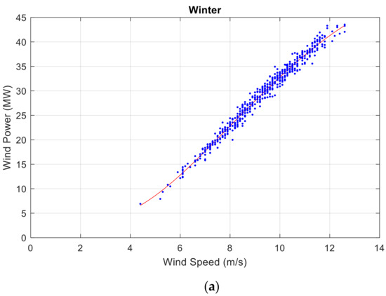
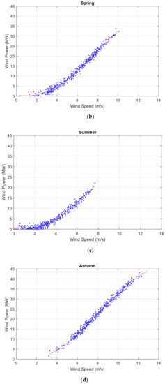
Figure 1.
The historical data available of the wind power: (a) wind speed and wind power in winter, (b) wind speed and wind power in spring, (c) wind speed and wind power in summer, and (d) wind speed and wind power in autumn.
2.1. Data Preprocessing
The wind power’s features and targets were normalized by min-max normalization. The inputs to the prediction model are shown in Figure 2. Three styles of inputs were present to the prediction model: (i) wind speed, (ii) temperature, and (iii) humidity. According to the prediction method, the generally used wind farm data selecting schemes were classified into two kinds, as described below.
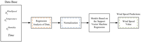
Figure 2.
Wind speed prediction model.
2.1.1. Wind Speed Prediction Process
Wind is strongly intermittent, and although making predictions is an extremely difficult problem, it is inextricably linked to the preparatory work for the construction of wind power prediction models. In this study, the input variables were temperature, humidity, and wind speed, while the output variables were the wind speed value in the next period. The support vector machine was used to make one-hour wind speed predictions and one-day wind speed predictions. Figure 2 shows the construction process of the wind speed prediction of the proposed model.
2.1.2. Construction of Power Generation Model
The actual power generation value often has a point where the power generation amount fluctuates greatly or a point where an abnormal value is caused by improper measurements of the instrument [19]. These power generation amounts act like “noise”, and this paper could perform data regression analysis twice. The cluster points constructed for the first time were used to explore all historical data, and the second time was based on the first cluster point to filter the data. Of the generated data, 20% of the data generated by each cluster distance from the cluster was deleted. The reference materials included in the data regression analysis were used to construct a more complete clustering point using the remaining data. The wind power process is given in Figure 3.
Figure 3.
Wind power modeling process.
2.2. Wind Power Generation
To capture the maximal wind energy, it is necessary to install the power electronic devices between the wind turbine generator and the grid in a location where the frequency is constant [24]. For a variable speed wind turbine, the output mechanical power of the wind turbine () can be described as:
where is the density of the air around the turbine, A is the turbine’s cross-sectional area, and is the wind velocity in m/s. In addition, is the power coefficient. The tip speed ratio (TSR) is found as:
where r is wind turbine blade tip radius and is the turbine angular speed. For a variable pitch angle wind generation system, the blade pitch angle is , and the TSR and power coefficient are defined as:
By Equation (3), the power coefficient curve was as shown in Figure 4. In a wind turbine, there is an optimum value of the tip speed ratio, which leads to the maximum power coefficient.
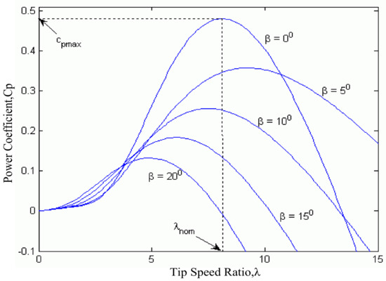
Figure 4.
Power coefficient curve of the wind turbine.
2.3. Performance Measurements
The mean speed of the wind (VMED), mean absolute error (MAE), root mean squared error (RMSE), and mean absolute percent error (MAPE), are widely used to assess the performance of wind power forecasting [25]. VMED is the average wind speed as follows:
MAE presents the accuracy in the same data units, which assists to conceptualize the magnitude of the error. It is represented in the following equation:
where N is the number of samples, is the actual speed, and is the predicted speed.
RMSE is easier to explain as it is indicated in the same units as the forecasted variable:
MAPE presents the accuracy as a percentage error. Because this number is a percentage, it may be easier to understand than other measure formulas. It is represented in the following equation:
3. Proposed Bee Swarm Optimization with Support Vector Machine Algorithm
Application of bee swarm optimization combined with data regression and least square support vector machine (DR-SVM) is an artificial intelligence pattern identification algorithm [22,23]. It is a new machine learning method based on the statistical learning theory. It has many unique advantages in solving problems due to a small sample size, as well as nonlinear and high-dimensional pattern recognition problems. It is used in practical problems such as handwriting recognition software, face recognition, and image classification. The bee swarm algorithm is a new optimization algorithm that can solve numerical optimization problems accurately and quickly, and which has the advantages of a simple concept, easy implementation, and fewer control parameters [26,27].
3.1. Least Square Support Vector Machine
In the field of artificial intelligence, support vector machines (SVM) are an artificial intelligence method that was proposed by Vapnik and AT&T laboratories in 1995 [28,29], in which the main theory is to use the structural risk minimization method in statistical learning. Support vector machines mainly use the separating hyperplane to distinguish two or more different types of data. In dealing with the problem of data exploration and classification, they have been used in many fields in recent years and have provided good results. Numerous scholars have studied and improved other methods, thereby making the application more extensive and the results more accurate.
In a typical classification problem, the following basic representation methods are usually defined:
- : A vector used to describe the style or attributes of a piece of data.
- .
- : The target, usually expressed as {±1} (assuming the target is divided into two categories), in which +1 and −1 indicate two different categories.
- .
The support vector machine is mainly used in classification and regression analysis. The proposed method uses its support vector classification and regression capability to simulate the fault location, type, and distance. The principle of the support vector machine is shown in Figure 5. The low-dimensional data of the input space are converted into a high-dimensional feature space. The data, which originally needed to be processed by a nonlinear curve, become a linear concept that can be easily processed.
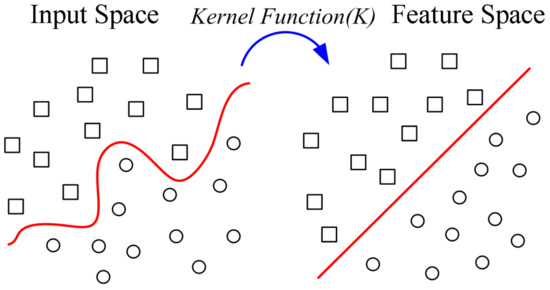
Figure 5.
Characteristics of spatial transformation.
The support vector machine used in the proposed method is the least square support vector machine (LSSVM), which has seen improvements in recent years. Its parameter setting is less than that of the traditional support vector machine, and there is no need to set the insensitivity parameter of ε. It is only necessary to set the adjustment parameter γ and radial core function K.
Support vector classification (SVC) mainly uses the hyperplane to separate data into two or more different categories, because the actual data may be high-dimensional data, and the hyperplane means the plane in high dimensions. As shown in Figure 6, linear classification is mainly used to find the hyperplane in the feature space to maximize the distance of the training data and then divide the data into two or more different types of data. It can be assumed that the hyperplane is , and is expressed as a vector used to describe each data characteristic attributes, [22,23].
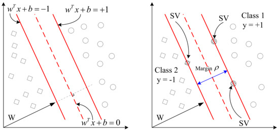
Figure 6.
Linear classification.
Suppose that the training data set is , in which represents an n-dimensional input vector and represents two types of data. The hyperplane can be used to classify the data set, and the maximum distance between the hyperplane and the two boundaries is called the maximum margin hyperplane.
The training data on the boundary are called the support vector (SV), and ρ is the maximum boundary. The classification curve is as follows:
If , can be expressed as:
If the training data satisfy the above formula, the maximum boundary can be obtained as follows:
From the above formula, the target letter can be obtained:
Since the objective function is a quadratic optimization problem, the Lagrange problem can be obtained from Equations (9) and (10) as follows:
Here is the Lagrange multiplier of the vector. According to the Karush–Kuhn–Tucker (KKT) conditions, the following formula can be obtained:
Substituting Equation (13) into Equation (12) obtains the objective function:
The support vector is the training data that satisfy the KKT condition, and these points will fall on the maximum boundary. After these support vectors are obtained, new data can be classified by the support vector. The mathematical concept of support vector regression (SVR) is as follows: the known training data set is , for input data, and output data. The linear regression objective function can be expressed as:
Adding Equation (14) to the error function containing ε insensitivity results in the following equation:
Introducing two slack variables, one for the target value higher than ε and the other for the target value lower than ε, results in:
From Equation (17), the following equation can be obtained:
From Equations (15), (16), and (18), the original optimization problem is obtained:
In which the smaller range of the error term is better. The adjustment parameter of the support vector machine represents the penalty weight for the error data of the support vector machine. In order to avoid the occurrence of over-matching, the parameter setting is particularly important. The output of the upper and lower measurement limits of the relaxation variable is shown in Figure 7.
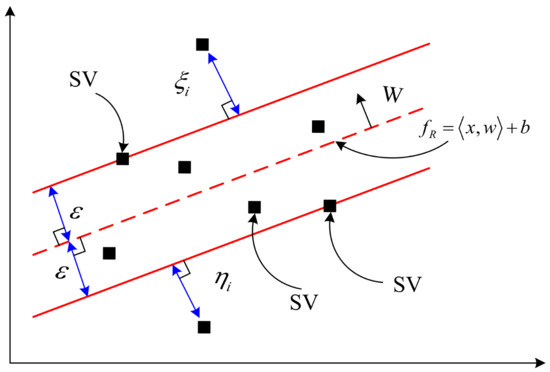
Figure 7.
Slack variables in the linear regression.
The support vector machine used in the proposed method is the least square support vector (LSSVM). The support vector machine has hyperplane parameter settings in the application, which are greatly affected by the number of training data, leading to the problem of an excessively large solution range.
The least square support vector machine mainly sets parameter ε to 0, making each item of data a support vector point to find the regression curve. Because the support vector machine solves the quadratic programming problem, the variable dimension is equal to the number of training data items; therefore, the number of matrix elements is the square of the amount of training data. When the scale of the data reaches a certain level, traditional mathematical rules will become difficult to deal with. The LSSVM method solves the linear equations to achieve the final regression curve, which reduces the difficulty of the solution to a certain extent and improves the speed of the solution.
This paper used the radial core function , and used the regression and prediction capabilities of LSSVM to construct the correlation between the data regression and the forecast. After selecting the modeling data through data regression, the support vector machine was used for training and modeling to realize the state structure of the predicted wind speed modeling. In terms of predicting the wind speed, the parameters of the input layer included temperature, humidity, wind speed, etc., and the least square support vector machine was used to predict the wind speed at the output layer. In terms of the power generation model construction, the input layer parameter was the wind speed, and the LSSVM was used for the output power generation. The wind power generation forecast error was normalized according to the actual wind speed interval and the capacity of the wind farm at the time of forecast, so as to reflect the true forecast accuracy.
3.2. Enhanced Bee Swarm Optimization Algorithm
In recent years, biological group intelligence has become one of the main fields of scientific research, and many optimization algorithms have been developed based on the concept of group intelligence, including the ant colony optimization algorithm, particles swarm optimization, and the bee swarm optimization; the concept of group intelligence is still widely used. The bee swarm algorithm can accurately and quickly solve numerical optimization problems by referring to the bee colony’s division mode and type. It has simple concepts, easy implementation, fast convergence speed, few parameter settings, and a wide search range [26,27].
The groups in the bee swarm algorithm are represented as worker bees, follower bees, and scouting bees. Improvements to the working model include: each bee colony determines its number first, unlike the artificial swarms of bees except the worker bees, and the groups will only join when needed, so as to ensure that all groups can participate in the overall search process. The random change of search direction was added to the working mode of each ethnic group to avoid falling into the local optimal solution. The working mode of each ethnic group was as follows:
- (1)
- Worker Bee Working Mode
The worker bee will search according to the current location, as shown in Equations (20) to (24). In addition, in order to avoid search areas that can be ignored, when the randomly generated rand value is greater than the set pr value, a reverse search is performed:
where
- j: The number of worker bee populations
- : The old nectar location.
- : The new nectar location.
- : The worker bee’s own cognitive ability.
- : The group cognitive ability of the worker bees.
- : A random number between 0 and 1.
- : The best search location for the worker bees themselves.
- : The best search location for the worker bee colony.
- : A reverse search judgment.
- : The maximum number of searches.
A certain number of worker bees in the worker bee colony executes Equation (25); randomly selects two groups, m1 and m2, from the solution of all bee colonies; and judges the working mode according to their fitness values, so that the worker bees will not be completely based on the best solution. The search can also be performed according to the second-best solution to increase the group diversity, assuming that this certain number is 30% of the number of worker bee groups:
- (2)
- Follower Bee working mode
The follower bees also use Equation (26) as a criterion to determine whether to follow the worker bees for food. They are not added to the worker bee group in the enhanced bee swarm algorithm, as they are only followers. In the follower bee working mode, a reverse search is also added to increase the search area:
where
- k: The number of follower bee groups;
- : A position randomly selected by the follower bee according to Equation (26) at the t-th iteration.
- (3)
- Scouting Bee Working Mode
The scouting bee is no longer an unfounded random search, and its working mode is changed to generate a new position after comparing the global best solution found by the t-th iteration with the average value of all group positions:
where
- s: The number of scouting bees.
- r: A random number between 0 and 1.
- : The average value of all group positions at the t-th iteration.
- round: Take the integer.
- The flow of the bee swarm algorithm is as follows:
- (a)
- Generate initial settings and data, including the maximum number of iterations, the number of groups, the number of variables, and the upper and lower limits. Generate the N group variable combination, calculate the fitness value of the variable combination , and record the best solution.
- (b)
- The worker bees conduct proximity searches.
- (c)
- Calculate the benefit rate of all variable combinations with as the probability and follow the bees using the roulette mechanism to randomly select a honey source for further searching.
- (d)
- The scouting bee generates a new position based on the comparison between the t-th iteration best solution and the group position average.
- (e)
- Repeat steps (a) to (d) to search the best solution in the whole area.
- (f)
- Determine whether the upper limit of the number of iterations is reached. If not, continue the iteration; if the upper limit is exceeded, output the result.
3.3. Wind Power Forecasting Process
The wind power forecasting process is mainly divided into three parts. The flow chart is shown in Figure 8.
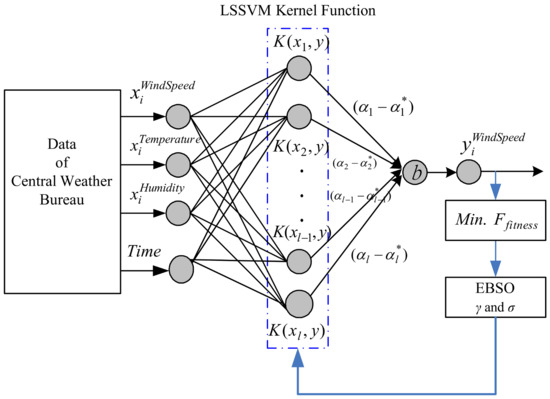
Figure 8.
Enhanced Bee Swarm Optimization with Least Square Support Vector Machine (EBSO_LSSVM) system architecture diagram.
- Part 1: Apply data regression analysis to select the modeling data.
- Part 2: Apply the bee swarm algorithm to solve the best setting parameters for the support vector machine.
As the support vector machine parameter selection has a great influence on the regression analysis, the parameter selection will often vary in different cases; therefore, the proposed method used the data regression support vector machine as the main body combined with the bee swarm algorithm, which was referred to as Enhanced Bee Swarm Optimization with Least Square Support Vector Machine (EBSO_LSSVM). The bee swarm algorithm was used to find better setting parameters for γ and σ in the support vector machine, and resulted in better training parameters, thus improving on the traditional shortcomings of unclear support vector machine parameter selection. The EBSO_LSSVM system architecture is shown in Figure 8.
- Part 3: Use EBSO_LSSVM to perform wind speed prediction.
4. Simulation Results and Analysis
The Central Weather Bureau data of wind power from December 2018 to November 2019 were taken from Yunlin County in Taiwan and were implemented using the computer CPU of the Intel Core i7-3770k 3.5 GHz and RAM of 8 GB for the MATLAB R2015a (Santa Clara, CA, USA). The data were publicly available for researchers on the Central Weather Bureau Automatic Weather Station’s website.
The DR-SVM model was compared with three other models, namely the conventional radial basis function (RBF) [30], SVM [31], and DR-RBF, for wind power prediction. In the case of the wind speed, data regression combined with the EBSO_LSSVM model was used for the forecast [32,33].
4.1. Short Term Wind Power Forecasting (Hours)
The generated power varied according to the expected wind speed for the wind farm. For this, the wind farm can generate power up to 45 MW. The expected short-term generated power results are presented in Figure 9. The variation in the power generation prediction behavior was smoother than that in the ultra-short prediction, but there was still a variation of approximately 10 MW at a range of eight to ten hours. The average output power of the proposed algorithm in the four seasons was better than that of the other methods, and the wind power in winter was higher compared to the other seasons. Furthermore, the DR-SVM model returned a higher accuracy than the other models.
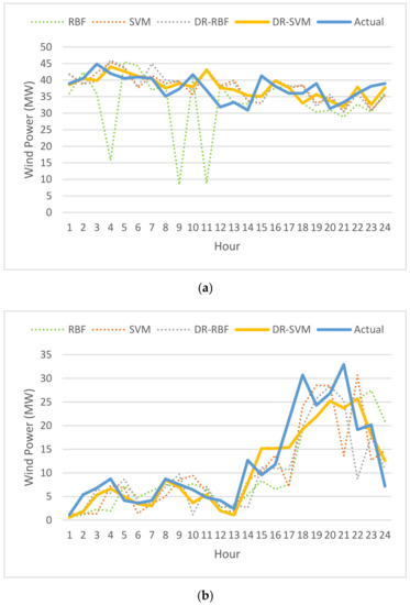
Figure 9.
Seasonal short-term wind power predictions: (a) winter; (b) spring; (c) summer; (d) autumn.
4.2. Ultra-Short-Term Wind Speed Forecasting (10 min)
The results of display the speed value in m/s prediction for the ultra-short term forecasting of 10 min are shown in Figure 10. As seen in Figure 10, there was little difference between the DR-RBF model and the DR-SVM model. The forecast was made from January 2019 to October 2019 during all four seasons. For the ultra-short term, the proposed DR-SVM model had better results than the other models. The momentary, randomness, and non-smooth aspects of the short-term wind speed allocation were significantly reduced, which was of great advantage to the improvement of the forecast accuracy. The proposed method could effectually combine the merits of different methods to effectually enhance the wind speed forecast accuracy.
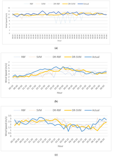
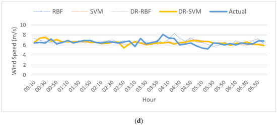
Figure 10.
Seasonal ultra-short-term wind speed predictions: (a) winter; (b) spring; (c) summer; (d) autumn.
4.3. DR-SVM Performance Evaluation
Four evaluation indicators were used for the performance evaluation of the wind power forecasting: VMED, MAE, RMSE, and MAPE, as shown in Table 1. MAPE, RMSE, and MAE have been widely used to evaluate the performance of wind power forecasting models. The results shown in Figure 9 and Figure 10 and in Table 1 were taken during a 24-h period in each season, i.e., 21 January (winter), 6 May (spring), 22 July (summer), and 21 October (autumn). According to the deterministic 1-h ahead forecasting error, the forecasting error for each season and for the average results was reduced by 6.86%, 15.31%, 15.90%, 9.39%, and 11.86%, respectively. The results shown in Table 1 indicated that the forecasting accuracy of the DR-SVM model was significantly better than DR-RBF and SVM, and that SVM was significantly better than RBF. Taking into account the accuracy of DR-SVM in winter, the forecasting accuracy was improved by 41.16%, 17.15%, and 14.35% in MAPE, referring to the preceding three methods, respectively. Moreover, the average forecasting errors of the proposed DR-SVM are shown in Figure 11. It is clearly seen that the wind speed forecasting has errors in all four seasons. Table 2 shows the average errors in the values of predicted speed for all season ultra-short term forecast. It can be seen that DR-SVM improves the searching capability with the best possibility of guaranteeing a global optimum. From Table 2, the DR-SVM algorithm demonstrates better accuracy, while the VMED, MAE, RMSE, and MAPE are greater than those in RBF [30], SVM [31], and DR-RBF.

Table 1.
VMED, MAE, RMSE, and MAPE of the proposed and compared methods.
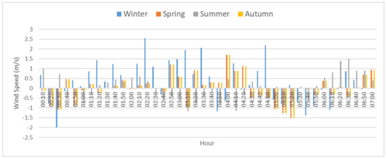
Figure 11.
Seasonal ultra-short-term wind speed forecasting error.
Table 2.
Results of errors for all season ultra-short term (min).
The simulation results show that the proposed method based on data regression and the enhanced support vector machine can effectually improve the prediction accuracy of short-term wind speed. Moreover, the usefulness of the proposed DR-SVM algorithm achieves both the objectives: improving wind power forecasting accuracy and reducing computational costs. The effectiveness of the algorithm is illustrated by performing optimization on some cases, and the results are compared to those in previous journals. Our results show that the proposed method is realizable, robust, and more valid than many formerly-established algorithms.
5. Conclusions
Wind energy is inexhaustible, and wind power can effectively slow down the consumption of energy resources. Its development trend is unstoppable. However, the existence of uncontrollable factors such as intermittent wind and random fluctuations represent a great challenge. Large-scale wind power grid integration will inevitably impact power system stability and cause the accurate forecasting of wind power to become a top priority. The accuracy of wind power forecasting depends on the method of constructing the forecasting model and the accuracy of weather forecasting. Faced with the advent of big data, the limited use of effective data can reduce resource consumption. Therefore, this paper proposed wind power forecasting based on data regression. Among the numerous artificial intelligence methods, support vector machines with their superior ability to process nonlinear characteristics were selected for regression.
5.1. Wind Speed Prediction
This paper used data regression to filter valid historical data so as to select useful similar data from the weather database, reduce the impact of invalid data, and effectively reduce the modeling time. This method was combined with the bee swarm optimization and support vector machine for prediction. It was used to adjust the relevant parameters to improve the prediction ability, so that the drastic data changes could be predicted more accurately, thus allowing it to effectively become a climate prediction model for wind power generation.
5.2. Construction of the Power Generation Model and Wind Power Forecast
Based on historical wind power data, this paper selected representative cluster power generation by data regression, clusters to a power generation for each wind speed interval of meter/second, and combined the EBSO and LSSVM. The construction of the power generation model not only effectively reduced the modeling time, but also increased the accuracy of the model in comparison to that of the LSSVM model. In terms of the wind power prediction, combined with the results of wind speed prediction, and using the power generation corresponding to the power generation model to obtain wind power prediction, the discussion and conclusions of the case analysis provided better prediction results.
Author Contributions
C.-S.T. performed the simulations, conducted the concept and planning the project. C.-M.H. contributed to the development algorithm and prepared the original draft of the manuscript to be submitted. H.-S.H. analyzed the wind model and data collection. C.-H.C. verified the prediction results. All authors discussed the results, analyzed the simulation data and approved the article. All authors have read and agreed to the published version of the manuscript.
Funding
This research received no external funding.
Acknowledgments
The authors would like to acknowledge the financial support for this work by the Ministry of Fuzhou Polytechnic of number RCQD201704 is gratefully appreciated.
Conflicts of Interest
The authors declare no conflict of interest.
References
- Landberg, L. Short-term prediction of local wind conditions. J. Wind Eng. Ind. Aerodyn. 2001, 89, 235–245. [Google Scholar] [CrossRef]
- Shao, H.; Deng, X. Adaboosting neural network for short-term wind speed forecasting based on seasonal characteristics analysis and lag space estimation. Comput. Model. Eng. Sci. 2018, 114, 277–293. [Google Scholar]
- Beyer, H.D.; Mellinghoff, H.; Monnich, K.; Waldl, H.P. Forecast of regional power output of wind turbines. In Proceedings of the European Wind Energy Conference, Nice, France, 1–5 March 1999; p. 1073. [Google Scholar]
- Landberg, L. Short-term prediction of the power production from wind farms. J. Wind Eng. Ind. Aerodyn. 1999, 80, 207–220. [Google Scholar] [CrossRef]
- Focken, U.; Lange, M.; Waldl, H.P. Previento–A wind power prediction System with an innovative upscaling algorithm. In Proceedings of the 2001 European Wind Energy Association Conference, EWEC’01, Copenhagen, Danmark, 2 July 2001; pp. 826–829. [Google Scholar]
- Xu, Q.; He, D.; Zhang, N.; Kang, C.; Xia, Q.; Bai, J.; Huang, J. A short-term wind power forecasting approach with adjustment of numerical weather prediction input by data mining. IEEE Trans. Sustain. Energy 2015, 6, 1283–1291. [Google Scholar] [CrossRef]
- Felder, M.; Kaifel, A.; Graves, A. Wind power prediction using mixture density recurrent neural networks. In Proceedings of the Poster Presentation Gehalten AUF DER European Wind Energy Conference 2010, Warsaw, Poland, 23 April 2010. [Google Scholar]
- Soman, S.S.; Zareipour, H.; Malik, O.; Mandal, P. A review of wind power and wind speed forecasting methods with different time horizons. In Proceedings of the 2010 North American Power Symposium, Arlington, TX, USA, 26–28 September 2010. [Google Scholar]
- Giebel, G.; Landberg, L.; Nielsen, T.S.; Madsen, H. The Zephyr-project. The next generation prediction system (poster). In Proceedings of the CD-ROM European Wind Energy Association (EWEA) 2002, Paris, France, 2–5 April 2002. [Google Scholar]
- Jorgensen, J.; Moehrlen, C.; Gallaghoir, B.O.; Mckeogh, E. HIRPOM: Description of an operational numerical wind power prediction model for large scale integration of on-and offshore wind power in Denmark. In Proceedings of the Poster on the Global Wind Power Conference and Exhibition, London, UK, 1 January–30 September 2002. [Google Scholar]
- Gu, X.; Wang, X. A review on wind power forecast technologies. Power Syst. Technol. 2007, 31, 335–338. [Google Scholar]
- Yan, J.; Li, K.; Bai, E.; Zhao, X.; Xue, Y.; Foley, A.M. Analytical Iterative Multistep Interval Forecasts of Wind Generation Based on TLGP. IEEE Trans. Sustain. Energy 2018, 10, 625–636. [Google Scholar] [CrossRef]
- Wang, L.; Yang, G.; Gao, S. A review on modeling and forecasting of wind power. Prot. Control Power Syst. 2009, 37, 118–121. [Google Scholar]
- Gong, W.; Meyer, F.J.; Liu, S.; Hanssen, R.F. Temporal Filtering of InSAR Data Using Statistical Parameters From NWP Models. IEEE Trans. Geosci. Remote Sens. 2015, 53, 4033–4044. [Google Scholar] [CrossRef]
- Carpinone, A.; Giorgio, M.; Langella, R.; Testa, A. Markov chain modeling for very-short-term wind power forecasting. Electr. Power Syst. Res. 2015, 122, 152–158. [Google Scholar] [CrossRef]
- Karadas, M.; Celik, H.M.; Serpen, U.; Toksoy, M. Multiple regression analysis of performance parameters of a binary cycle geothermal power plant. Geothermics 2015, 54, 68–75. [Google Scholar] [CrossRef]
- Cadenas, E.; Jaramillo, O.A.; Rivera, W. Analysis and forecasting of wind velocity in chetumal, quintana roo, using the single exponential smoothing method. Renew. Energy 2010, 35, 925–930. [Google Scholar] [CrossRef]
- Babazadeh, H.; Gao, W.; Cheng, L.; Lin, J. An hour ahead wind speed prediction by Kalman filter. In Proceedings of the 2012 IEEE Power Electronics and Machines in Wind Applications, Denver, CO, USA, 16–18 July 2012. [Google Scholar]
- Zhang, J.; Wang, C. Application of ARMA model in ultra-short term prediction of wind power. In Proceedings of the International Conference on Computer Sciences and Applications, San Francisco, CA, USA, 23–25 October 2013. [Google Scholar]
- Tagliaferri, F.; Viola, I.M.; Flay, R.G.J. Wind direction forecasting with artificial neural networks and support vector machines. Ocean Eng. 2015, 97, 65–73. [Google Scholar] [CrossRef]
- Wang, X.; Zheng, Y.; Li, L.; Zhou, L.; Yao, G.; Huang, T. Short-term wind power prediction based on wavelet decomposition and extreme learning machine. In Proceedings of the Advances in Neural Networks 9th International Symposium on Neural Networks, Shenyang, China, 11–14 July 2012. [Google Scholar]
- Zhang, Q.; Lai, K.K.; Niu, D.; Wang, Q.; Zhang, X. A fuzzy group forecasting model based on least squares support vector machine (LS-SVM) for short-term wind power. Energies 2012, 5, 3329–3346. [Google Scholar] [CrossRef]
- Zeng, J.; Qiao, W. Short-term solar power prediction using a support vector machine. Renew. Energy 2013, 52, 118–127. [Google Scholar] [CrossRef]
- Lin, W.M.; Hong, C.M.; Chen, C.H. Neural-network-based MPPT control of a stand-alone hybrid power generation system. IEEE Trans. Power Electron. 2011, 26, 3571–3581. [Google Scholar] [CrossRef]
- Alencar, D.B.; Affonso, C.M.; Oliveira, R.C.L.; Rodríguez, J.L.M.; Leite, J.C.; Filho, J.C.R. Different models for forecasting wind power generation: Case study. Energies 2017, 10, 1976. [Google Scholar]
- Karaboga, D.; Basturk, B. A powerful and efficient algorithm for numerical function optimization: Artificial bee colony (ABC) algorithm. J. Glob. Optim. 2007, 39, 459–471. [Google Scholar] [CrossRef]
- Taher, N.; Faranak, G. Enhanced bee swarm optimization algorithm for dynamic economic dispatch. IEEE Syst. J. 2013, 7, 4. [Google Scholar]
- Cortes, C.; Vapnik, V. Support-Vector Networks. Mach. Learn. 1995, 20, 273–297. [Google Scholar] [CrossRef]
- Burges, C.J.C. A Tutorial on Support Vector Machines for Pattern Recognition. Data Min. Knowl. 1998, 2, 1–47. [Google Scholar]
- Chang, W.Y. Wind energy conversion system power forecasting using radial basis function neural network. Appl. Mech. Mater. 2013, 284–287, 1067–1071. [Google Scholar] [CrossRef]
- Zhou, J.Y.; Shi, J.; Li, G. Fine tuning support vector machines for short-term wind speed forecasting. Energy Convers. Manag. 2011, 52, 1990–1998. [Google Scholar] [CrossRef]
- Deng, X.; Shao, H.; Hu, C.; Jiang, D.; Jiang, Y. Wind power forecasting methods based on deep learning: A Survey. Comput. Model. Eng. Sci. 2020, 122, 273–301. [Google Scholar] [CrossRef]
- Sana, M.; Turki, A.A.; Sameeh, U.; Aisha, F.; Nadeem, J.; Tanzila, S. Exploiting deep learning for wind power forecasting based on big data analytics. Appl. Sci. 2019, 9, 4417. [Google Scholar]


Publisher’s Note: MDPI stays neutral with regard to jurisdictional claims in published maps and institutional affiliations. |
© 2020 by the authors. Licensee MDPI, Basel, Switzerland. This article is an open access article distributed under the terms and conditions of the Creative Commons Attribution (CC BY) license (http://creativecommons.org/licenses/by/4.0/).