Abstract
Electricity distribution network optimisation has attracted attention in recent years due to the widespread penetration of distributed generation. A considerable portion of network optimisation algorithms rely on an initial solution that is supposed to bypass the time-consuming steps of optimisation routines. The aim of this paper is to present a nature inspired algorithm for initial network generation. Based on slime mold behaviour, the algorithm can generate a large-scale network in a reasonable computation time. A mathematical formulation and parameter exploration of the slime mold algorithm are presented. Slime mold networks resemble a relaxed minimum spanning tree with better balance between the investment and loss costs of a distribution network. Results indicate lower total costs for suburban and urban networks.
1. Introduction
The increase of renewable energy production has raised a lot of concerns about the capability of distribution networks to host distributed generation. The shift towards bi-directional power flows in distribution networks set new demands for planning algorithms that are able to cope with new requirements of network operation strategies. Due to the complexity of planning tasks, the significance of a good quality starting point for an optimisation process cannot be overestimated.
Power system planning is a complex optimisation task. The nonlinear nature of power flow equations can be relaxed or substituted with convex equivalents [1]. The binary nature of network connections, however, has still no workaround. Topology optimisation, as any other combinatorial optimisation, is inherently computationally demanding in finding the global optimum for a large system. Numerous attempts to solve the network topology problem have been addressed in works employing mathematical and heuristic programming. A second-order cone programming formulation for distribution network reconfiguration was utilized in [2,3]. A similar formulation was employed in [4] to include active network expansion planning under different scenarios. A multi-objective seeker-optimisation heuristic algorithm was proposed in [5] for optimal design of distribution network. A scenario-based expansion planning with genetic algorithm optimization was presented in [6]. The authors of [7] propose a hybrid Tabu search and particle swarm optimization to address medium-voltage network expansion planning. Heuristics provide a trade-off between accuracy and computation time. Despite the advantages, heuristics cannot guarantee to reach the global solution. Due to that reason, mathematical programming tools are still preferred by a large number of researchers.
The importance of warm-starting an optimisation algorithm with an initial solution has been emphasised in several works. The authors in [3] have stated that convergence time can be greatly accelerated if a good starting solution is provided. Likewise, Ref. [2] has stated that an initial solution for a mixed-integer problem can save time for a later stage of branch-and-cut of the search tree that would help optimization to reach the optimum in a smaller number of iterations. Authors of [8] highlighted a promising field for initial topology generation. A warm up strategy is utilized in [9] to prune inactive edges of a network topology and reduce the search tree. Most solvers have built-in heuristics to guess a feasible starting point, but the actual routine of generating an initial solution is beyond the user’s control.
Somewhat naturally, network planning often involves an expansion of existing networks. An expansion by reconfiguration of network connections was presented in [10]. Similarly, an expansion planning for multistage problem with simplified objective function was shown in [11]. An optimal utilization of connection boxes within an existing network was presented in [12]. Possible new connections are added to predefined corridors, while keeping the rest of the network untouched. This way, the number of options is limited, thus cutting computation time and giving predictable solutions. A topology optimisation method based on a branch-and-bound algorithm was developed in [8]. Even though the method was not dedicated specifically for initial network generation, the authors highlighted its potential warm-starting enhanced algorithms. The method was showcased on a realistic network from Brazil; however, it was scaled down to several hundreds of nodes. The initial network problem was addressed in [13]. It is based on node topological information and is easy to implement as no demanding computation is involved. Still, it considers reconfiguration of existing networks with given tie switches at fixed locations. The scalability of the presented method is great. Nevertheless, the given possible tie switch locations lessen the work for the algorithm.
An algorithm in [14] modifies the minimum spanning tree (MST) to reduce the optimality gap and take the objective closer to the optimal solution. In the cornerstone of the algorithm lies the assumption that by relaxing the radiality constraint, thus adding extra node connections, a better objective value can be achieved. The method provides an efficient solution and is scaled up to hundreds of nodes. The method covers reconfiguration of an existing network, but as with all the works mentioned above, it does not demonstrate a case with greenfield planning.
Greenfield planning implies no predefined connection options in a planning task, which leaves an enormous number of possible connection combinations. To narrow down the feasible region in greenfield planning, meshing techniques can be employed. Most widely used is the Delaunay triangulation, which sets predefined connection paths in a mesh-like structure. A network is optimized by a combination of steepest descent and simulated annealing in [15]. The available connections were predefined and constituted a mesh-like structure to initialize the optimization process. A network optimization by bacterial foraging algorithm was initialized by a triangular mesh of a network in [16]. In [17], the candidate nodes and lines are prioritized and the topology is found by dynamic programming, with the following relocation of some predefined nodes to improve the objective value. In a densely populated city environment, a street grid was adopted as a starting ground for a network in [18]. However, many prefer to use the advantage of warm-start capabilities of other methods. The vast majority of warm-start initial networks are based on the MST. Genetic based algorithms use a chromosome coding, such as the Prüfer sequence, which represents a spanning tree, and the population is a set of feasible spanning trees [19]. Additionally, the MST was employed in [20,21] to create a set of feasible network topologies as initial populations for genetic algorithms. A multistage expansion planning algorithm demonstrated in [22] utilized an MST to construct a radial network for the medium-voltage stage of the distributed network optimization. A spatial optimization algorithm in [23] utilizes MST as an initialization topology for further search of the Steiner point. The Prim’s or Kruskal’s algorithms are commonly employed for MST generation, and just a few attempts to improve it hints that most of the researchers are satisfied with it.
The general idea of initial network generation remains in the shade of the MST dominance. Nevertheless, a few authors have proposed alternatives. An initial network generator was presented in [24]. Load nodes are divided into sectors around each feeding substation. Feeders are formed that connect each node within each sector with a minimum cost algorithm that utilises an approximate power flow based on the not-yet-connected remaining demand of the sector. The number of sectors are then progressively increased to find the minimum of the total cost that complies with the technical constraints.
The authors of [25] proposed an optimisation algorithm, in the base of which lies a clustering of load nodes. The nodes are spatially clustered into groups with similar power demand. The topology within each cluster is then found based on reliability requirements, and the feasibility of the topology is validated. The method is easily scalable up to large number of nodes, but, in essence, it divides the network into a number of small networks and still relies on the MST.
The MST is easy to understand and implement, but it minimises only the length of a network. The other crucial components of the total cost, such as loss costs and others, are neglected. On the contrary, the method proposed in [26] prefers to start from the other extreme, a star-like topology. Load nodes are connected to the feeding point via straight lines. The investment costs are sacrificed in order to gain the smallest loss costs but guarantees technical compliance in an initial network that is far from optimal. However, in real life cases, the optimal topology lies somewhere in between. The proposed method finds a balance between the MST and the star-like topology.
The main contribution of this paper is to present a new algorithm for an initial network generation for the greenfield design of a large-scale distribution network. The proposed algorithm addresses the disadvantage of MST, a widely used initial network type, and demonstrates the advantage of MST relaxation. Compared to the MST, the proposed algorithm can step back from the greedy approach of the MST and sacrifice shortest connections, in order to gain more from reduced loss costs. The algorithm is based on a slime mold organism, and its behaviour on a plane with spread out food sources. The slime mold algorithm can optimise networks with a large number of nodes with multiple sources and multiple sinks under a single simulation. It fills the gap in the algorithms that do not require fixed connections and can manage an enormous number of connection combinations in reasonable computation time. Such characteristics are beneficial for an initial network solution that is closer to the optimal as compared to other commonly used algorithms. The slime mold, which to the best knowledge of the authors, has not been used for this purpose, paves the way for new nature inspired heuristic algorithms that have been useful for topological problem-solving before.
The rest of the paper is organised as follows: the electric distribution network planning problem formulation is described in Section 2. Mathematical formulation of the slime mold and its parameter exploration are introduced in Section 3. Section 4 provides alternative algorithms for comparison simulations. The simulation results of realistic and synthetic networks are presented in Section 5, followed by a discussion in Section 6. Section 7 concludes the paper.
2. Problem Formulation
A distribution network can be defined as a set of nodes linked via connections. The set of nodes consist of load and substation nodes. The number of nodes is denoted by n and the number of substation nodes by . Each node has parameters such as x- and y coordinates, and estimated maximum load . The connections between the nodes are denoted in an adjacency matrix . For the presented problems, none of the fixed connections are defined; each node i can be connected to any other node j. The radiality condition of considered networks are granted by limiting the number of connections to . With the exception of small rural cases, networks are built in a meshed structure. However, they are operated in a radial topology and the unused links are utilized as back-ups. The cost function of an initial network consists of investment and loss costs:
The investment cost (2) includes the annuity factor , connection length , cable cost and binary directed adjacency matrix . The loss costs formulated in Equation (3) include annuity as well as the lifetime factor , cost of energy losses , loss utilisation time , cable resistance and current flow . For more detailed description of and , please refer to Appendix A. The rest of the simulation parameters have generalized realistic values based on authors’ experience in network planning in Finland, and are listed in Table 1.

Table 1.
Simulation parameters.
The simulations are carried out on two sets of networks: realistic networks and synthetic networks. The realistic networks are based on distribution networks in Finland. Due to confidentiality reasons, nodal data are falsified. The synthetic networks are randomly generated sets of nodes. The scale of network area, number of nodes and estimated average loads are based on typical Finnish networks, developed in [27]. Load nodes are placed on a plane in a random manner. The location of substation nodes is determined by the k-means clustering algorithm. Load nodes are clustered into a number of clusters that is equal to the number of substations, where the centroids represent substation locations. Table 2 includes the parameters of synthetic networks.
Table 2.
Network types.
3. The Slime Mold Algorithm
In the foundation of the proposed algorithm lies the behaviour of a slime mold organism Physarum polycephalum, later referred to as slime mold. It is a large yellow single-celled organism that can be found in cool and moist locations over a broad geographical range. Once deployed to some place, it starts to grow in all directions in search of a food source. The growing slime is spread in a thin layer to cover larger areas. Once a food source is found, the slime is concentrated around it in a thicker layer. Once two or more food sources are found, the slime mold forms a tubular network with conducting tubes to transport nutrients over the whole organism. Thicker tubes between food sources are formed, while the slime in previously searched areas decays. The slime mold constructs the tubes connecting food sources via shortest paths [28].
3.1. Slime Mold Application Areas
Slime mold got a lot of attention after it was proven to solve a maze. It was demonstrated that the slime mold algorithm can neglect dead-ends in a maze and choose a shorter path from several alternative ways [29]. A Steiner tree construction ability of the slime mold was then noticed and studied in [30,31]. Construction of a Steiner tree is an important network optimisation problem that is similar to the construction of the MST.
Additionally, the slime mold algorithm was employed in the optimisation of topological problems. Most of the works done are from the field of transportation. Notable results have been accomplished in modelling the Tokyo railway system [32,33]. A clever utilisation of the algorithm led to stunningly close to real-world network performance in terms of routing and fault tolerance. Similarly, the motorway networks of several countries have been modelled [34]. Once again, the resulting networks showed similarity to existing motorways. Supply chain optimisation by slime mold was introduced in [35]. Power system planning has only briefly touched the topic so far. The load-shedding of electricity demand by the slime mold was studied in [36]. The analogy of slime mold behaviour and power networks was briefly presented in [37].
3.2. Slime Mold Model
The model is inspired by food transportation within a slime mold. A distribution network is represented as a graph with food sources and tubes as nodes and connections, respectively. The tubes conduct fluid with nutrient, which is pushed by the pressure difference between each node. Let the pressure at node i and j be and , and the flux of the fluid through the tube with conductivity and length . Then, as in [29], we have
The nodes are divided into sink and source nodes, which represent load and substation nodes, respectively. Each sink node has a flux demand of and each source node supplies to the system the total demand divided by the number of source nodes. Over the course of simulations, the flux demand value was set to . The same value yielded a remarkably similar topology to the real Tokyo railway network in [32], as was mentioned previously. However, the effect of the flux demand value on the result still requires further analysis, as some applications alter the value and treat it as an input parameter [38]. According to Kirchhoff’s law, the total flux at each node is conserved, keeping the net flux at the rest of the nodes equal to zero. The balance of flux between several source and sink nodes is formulated in Equation (5) as in [35]:
The adaptive network formation was described in [29] by the difference Equation (6). The tube conductivity reacts to the flux by gradually shrinking the tubes without flux and expanding the conducting tubes. Input parameters and are the flow feedback rate and tube decay rate. The tube thickness response is calculated at each iteration k:
Equations (4) and (5) for all the nodes and tubes form a system of linear equations, which is solved at each iteration k and pressure p-values are obtained [29]. Furthermore, by securing the pressure value for reference nodes , the solution of (4) will result in a unique pressure value for every node. Assuming that tube conductivity and its length constitute a matrix , the vector of nodal pressure values can be solved by using the backslash operation in MATLAB as shown in (7):
Matrix is formed from matrix after reconfiguration of its diagonal and off-diagonal elements, as presented in Equation (8):
The simulation is initialised with tube conductivities equal to one. During the simulation, the conductivity values of decaying tubes will converge to zero and tubes that survive foraging will converge to a positive value. All the tubes that converge to a positive value constitute the final topology and form an undirected adjacency matrix of a solution. The flowchart of the algorithm is depicted in Figure 1.
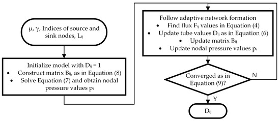
Figure 1.
Flowchart of the slime mold algorithm.
Slime mold solution requires calculations over a range of iterations to converge. The convergence criterion is based on the pressure matrix. Once the pressure difference between the previous and current iteration is lower than , the slime mold algorithm is considered to have converged (9):
The criterion for relative pressure difference is set to . Such a value grants simulation execution while the pressure difference between two consecutive iterations will be bigger than one percent. Other values were tested in search of a higher difference value that would return credible results in a smaller number of iterations. Nevertheless, values larger than one percent did not provide simulation convergence. Values smaller than that converged to the same result all the time but exploited a higher number of iterations. The results of convergence analysis are brought up in Table 3.
Table 3.
Number of iterations until convergence (blank values denote no convergence).
Even though slime mold has a functionality to exclude certain connections from a feasible region by multiplying the right-hand-side of (4) by a binary mask variable, the feature was left unused. Delaunay triangulation (triangular mesh), Gabriel graph and n-closest nodes were tested to propose candidate connections, but no increase in computation performance nor improvements on the results were recorded.
A strategy to enhance the computation efficiency of the slime mold algorithm is applied by finding and eliminating inactive nodes as indicated in [9]. Eliminating inactive nodes means that nodes that are not active in the network formation (e.g., dead ends, unused tap boxes) can be excluded from the slime mold solution. If a node is not a part of a network, the tubes that lead to that node will converge to zero, as (6) implies. Once that happens, the node pressure will drop to zero and then it is indicated as an inactive node. Inactive nodes are found continuously over the course of convergence and are excluded from the solution, making the system of linear equation calculation (7) faster.
3.3. Sector Based Slime Mold
The slime mold algorithm finds the shortest path between nodes, thus it considers only the distance between the nodes, other parameters, such as the load for example, are neglected. This can lead to a network solution where a group of nodes is connected to an overloaded feeder. Feeder capacity constraint has no representation in the slime mold algorithm at this stage. A method to cluster the nodes into sectors is proposed to add more feeders outgoing from substations and even up the load between them.
Firstly, node angles are found by measuring an angle from the y-axis, where a substation is in the origin of the plane. However, due to the angular gap between 0 and radians, the nodes that are close to each other on a plane may be allocated to different clusters. To overcome this problem, the angle reference point is rotated from the y-axis to the node with the biggest angular gap between consecutive nodes. Finally, the nodes are clustered over angles by one-dimensional k-means clustering.
The number of clusters, however, is not known. The criterion for the number of clusters is set to keep a feeder load from exceeding the cable ampacity . The number of clusters starts at one and is increased until the feeder capacity is not violated. Such a routine will divide nodes into sectors resembling slices of a cake. After the nodes are clustered, the slime mold optimises each cluster separately, and finally makes up the network topology.
3.4. Parameter Exploration
In order to reach a sub-optimal solution, the input parameters should be explored. As mentioned before, the slime mold algorithm finds the shortest path between nodes, so that the network solution gradually approaches MST. However, by relaxing the parameters, the topology can step back from the MST (Figure 2a) towards the star topology (Figure 2c). A balance between the smallest total length and smallest loss costs can be achieved as shown in Figure 2b.
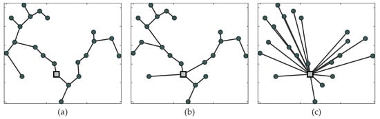
Figure 2.
Topology types (a) MST, (b) Slime Mold solution, and (c) Star topology.
In order to achieve a suitable topology, the input parameters: flow feedback rate and tube decay rate must be explored to obtain a balanced spanning tree. Typically, a desired result corresponds to a rather high and low , while the intervals of the two are and . The flow feedback rate is the main parameter that governs tube formation dynamics [37,38]. Values of lower than one will prevent the model from convergence, leaving many alternative connections between sink and source. Exceeding the upper bound will result in breaking some of the node connections, leaving some of the sink nodes disconnected. The upper limit of , however, can vary slightly depending on the size of the network. The tube decay rate has an opposite effect on the slime mold dynamics. A value of around the upper bound will result in a star topology with direct connections between source and sink nodes. By decreasing , the network topology will gradually approach the MST. The tube decay rate is characterised in [39] as the light-avoidance behaviour of slime mold organism and it affects the result to a great extent. The heatmap of the total cost dependency on the input parameters can be seen in Figure 3, where the cost is normalised by the cost of the MST of the network shown in Figure 2. The NaN values on the top-left corner of the plot indicate that the model did not converge.
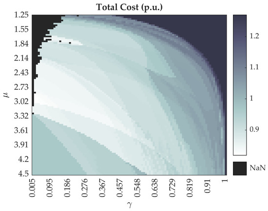
Figure 3.
Heatmap of the total cost dependency on the input parameters.
The split of normalized costs of the previously considered network can be seen in Figure 4. With one cable size considered, the investment cost grows linearly with the increased total length of a network. The loss costs, however, have a nonlinear dependence on the total length. The loss costs are smallest at the star-like topology and increase in an abrupt manner when approaching the MST. Typically, the lowest cost is close to that of the MST, but not exactly.
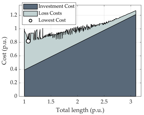
Figure 4.
Total cost split of the network.
4. Comparative Simulation
Other algorithms are utilised to provide a performance comparison of the slime mold algorithm, and are described below.
4.1. Prim’s Algorithm
Prim’s algorithm is a well known way to generate the MST. The Prim’s algorithm entails the greedy approach, which means that the next decision is made based on the smallest cost among available options. It is simple to implement and fast to simulate. A brief description of the algorithm is as follows:
- Nodes are divided into two sets: connected and non-connected nodes.
- The algorithm initialises by adding substation nodes into the set of connected nodes.
- Find node i from the set of non-connected nodes that is closest to any node from the connected node set.
- Connect the closest node i to the closest node from the set of connected nodes.
- Transfer node i from the set of non-connected nodes to connected nodes.
- Repeat steps 3–5 until the set of non-connected nodes is empty.
4.2. Mixed Integer Quadratic Programming
To provide a comparison with the slime mold and visualize the global optimum, a Mixed Integer Quadratic Programming (MIQP) model is used. The MIQP is only applied in the case of rural networks with a low number of nodes due to its high computation time. Presented below is a simplified model of the power flow equations presented in [1]. The objective is to minimise the total cost function of Equation (1), while the formulation of constraints is as follows:
is a binary directed adjacency matrix and M is a big M constant, is the power generated at node i, the power demand at node i, the power transfer from node i to j, the current flow from node i to j, and v the nominal voltage (assumed to be equal for all nodes). All variables, except for the binary variable , are continuous positive variables.
Equation (10) formulates the minimisation of the network total cost. Equation (11) enforces active power balance at all nodes: the net generation at a node should be equal to the net export from the same node. The current at every branch is calculated by (12). The limit for current flow in a line is set by (13). In case the connection is absent, , then the current flow is restricted. Otherwise, the constraint is relaxed by the big M, and current can pass. The numerical value of M is set to be equal to . The radiality constraint is enforced by (14). Equation (15) restricts power generation at load nodes, leaving the power generation to substation nodes only. For the sake of simplicity, a unity power factor is assumed.
4.3. Network Planning Algorithm Developed at Aalto University
A Network Planning Algorithm (NPA) has been developed at Aalto University, and it has an initial network generator included in its more extensive optimisation routine [24]. In tandem with the initial network generation, a full network is formed based on each sector-based underlying radial network and simple branch exchange routines are also run to locally optimise each intermediate solution, but this is not done in the comparisons for this paper. The aim in this paper is to provide a comparison of other sectoring methods with slime mold to produce an underlying radial initial network, without any further optimising tools. It should also be noted that the NPA runs a load flow for the cost calculation rather than load summation, as in the rest of the algorithms.
5. Results
In this section, the slime mold network optimisation example is shown and a comparison to other algorithms is presented. The comparison will showcase the computation time with respect to minimum cost. The slime mold and Prim’s algorithms were programmed in MATLAB R2020a, while the MIQP formulation of the problem was programmed in GAMS, a high-level modeling language that was launched via MATLAB interface. The CPLEX solver was selected because of its ability to efficiently reach the global optimum and provide an optimality gap value. The NPA was professionally coded in C/C-sharp and, due to security reasons, was simulated on another workstation. The computation time comparison of NPA is not fair in such a case; however, it is still added as a comparison to an established optimisation algorithm. The rest of the algorithms were simulated on a workstation equipped with an Intel Xeon 3.40 GHz processor and 16 GB of RAM.
5.1. Realistic Network
The realistic network presented is a falsified real-life network. Locations and load data are intentionally altered in order to secure the anonymity of customers. Despite the alterations, realistic networks accurately represent real-life network planning tasks. The 330-node network is pictured in Figure 5. The annual cost of the slime mold solution is kEUR, which splits into kEUR of investment cost and kEUR of loss costs. The MST of the Prim’s algorithm resulted in higher total cost that is kEUR of investment and kEUR of loss costs.
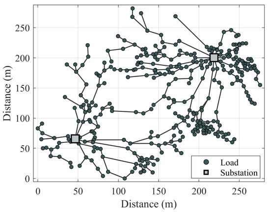
Figure 5.
Results of the sectored slime mold in realistic network cases.
5.2. Synthetic Networks
Furthermore, the slime mold algorithm is compared with the aforementioned algorithms utilising synthetic networks. Seven different network sizes are represented by ten random sets of nodes for each network size. The following figures provide a brief illustration of the network cost of each algorithm averaged over ten networks. In addition to average values, scatter plots illustrate the computation time of each network with respect to the actual network cost. Costs are normalised by the corresponding sectored slime mold values.
5.2.1. Rural Networks
The results of rural networks are shown in Figure 6a, where costs are normalized by the corresponding result of the Slime Mold sector. At a low number of nodes, all algorithms and their variations show similar cost values. The MIQP model represents the global minimum, which is reflected in the lowest cost in all the cases, as well as on average. Slime mold delivers worse results compared to the Prim’s MST. At the smallest network size, the optimal topology is equal to the MST, and slime mold relaxation of the MST yields no benefits. However, once the number of nodes in a network start to increase, the benefit starts to be noticeable. Moreover, the expediency of initial solutions in the case of such small networks is questionable. Modern computers and optimisation tools will reach the global optimum in a reasonable time.
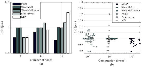
Figure 6.
Average cost of rural networks (a), and the cost and the computation time of each network (b).
The difference in slime mold and its sectored counterpart is negligible. With a lower number of customers, the feeder capacity is far from being exceeded. The clustering algorithm treats a full network as one cluster, thus sectored slime mold is identical to “pure” slime mold. A big difference in computation burden can be noticed on the scatter plot of Figure 6b. Three distinct clusters can be seen, where Prim’s and the slime mold are separated by two orders of magnitude of time. The MIQP model lies two orders of magnitude farther from slime mold, requiring around a second to find a global optimum for a network.
5.2.2. Intermediate Networks
The number of nodes is increased up to 41 in the intermediate networks. Starting from such a scale, the advantage of sectored slime mold is starting to become evident (Figure 7a). The number of customers in intermediate networks is big enough to overload a single feeder. The clustering algorithm divides loads into at least two sectors, creating a feeding cable for each. The disadvantage of MST starts to stand out at this size of network, as the Prim’s algorithm shows a 10% higher cost on average. The unsectored Prim’s algorithm was left out from the comparison due to poor results.
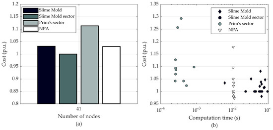
Figure 7.
Average cost of intermediate networks (a), and the cost and the computation time of each network (b).
The MIQP model was left out of the comparison as well due to unbearable computation time. As mentioned in [1,3], the computation time can be significantly reduced by accepting a slight offset from the global optimum. The first test network from the ten intermediate networks is optimised by the MIQP solver to observe the global optimum. Unfortunately, after 48 hours of computation, the CPLEX solver of the MIQP problem could not reach the global optimum and stopped at the optimality gap of 5.19% with respect to the optimal solution. Still, the value of the objective at that stage was lower than any other algorithm delivered, having a value of 95.4% of the sectored slime mold.
The general trend of computation time for intermediate networks remained the same as in the case with rural networks. Both of the slime mold algorithms perform at around the same time frame, while the Prim’s is faster (Figure 7b).
5.2.3. Urban Networks
The normalized results of urban networks, as shown in Figure 8, indicate that the sectored slime mold produces a network with lower cost when compared to Prim’s MST. The computation time of the sectored slime mold is, however, still higher than the other initial network generating algorithms: three orders higher than Prim’s algorithm and one order higher than NPA. The cost of the networks generated by the “pure” Slime mold are 50% higher than that of sectored slime mold, and, therefore, it was left out from the comparison.
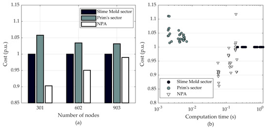
Figure 8.
Average cost of urban networks (a), and the cost and the computation time of each network (b).
Finally, computation times of the synthetic networks are summarized in Table 4. Computation times of the algorithms are averaged over the ten sets of nodes and divided into bins by the number of nodes in the network. The sectored Prim’s algorithm is faster in all the cases. Even though the slime mold is slower, it is as resilient in all the network sizes as the main competitors.
Table 4.
Averag computation times of each algorithm split by network sizes.
6. Discussion
As mentioned before, Steiner tree generation is a next level in optimal network design. A Steiner point can be easily interpreted as a cable box in low-voltage electric distribution networks. A cable box is a special case node that has no load and can be neglected from the final solution if it is not cost efficient to use one. Steiner point determination walks hand-in-hand with a routing application. The functionality of slime mold allows it to be employed in routing problems. A Euclidean space is divided into a grid of nodes that are interlinked in a mesh-like manner. The cost of each edge can be represented by a product of length and penalty of an underlying terrain. The routing capabilities of slime mold are inferior to Dijkstra due to the longer computation time. However, combined with the Steiner tree problem, slime mold has the potential to be employed in distribution network planning.
Due to the increased local generation of electricity in distribution networks in recent years, feeder capacity and voltage limits have received much attention in network planning applications [40]. For high quality initial network generation, slime mold must address such constraints. Workarounds, such as sectoring a set of nodes, can be of assistance. However, the slime mold algorithm would greatly benefit from feeder ampacity constraint. That could be possibly implemented by limiting the value of the flux in a tube, forcing flux to find an alternative path and form a new tube. Along with the feeder ampacity, a pressure drop constraint would greatly improve the quality of the slime mold networks. As an electricity distribution network must deliver a voltage level within acceptable bounds, the slime mold algorithm would greatly benefit from functionality to limit the pressure drop. Tube conductivity could compensate the pressure drop along a line, thus keeping pressure within limits. Future research in advancement of the slime mold algorithm would be highly welcomed.
7. Conclusions
The novelty of this paper is the application of the slime mold algorithm to the generation of initial network solution. The networks are generated for greenfield planning with no fixed candidate connections, thus leaving enormous search space for the algorithm to tackle. Slime mold is presented in two different variations: full network and sectored network optimisation. Additionally, slime mold behaviour and input parameter exploration is described.
The slime mold algorithm is compared with the most common initial network type, the MST. It is revealed that the utilization of the slime mold algorithm pays off in the case of suburban and urban networks. The slime mold solution, which represents a relaxed MST, yields beneficial reduction of loss costs and lower network cost overall. The slime mold algorithm demonstrates up to a 10% lower cost compared to MST on average. On the other hand, the computation time of the MST is hard to compete. Simple implementation of the greedy approach was at least two orders of magnitude faster. Still, even the slowest slime mold solutions for the largest networks were achieved in just few seconds. In conclusion, network optimization problems that are looking for a good initial solution would benefit from the slime mold algorithm. The advantage of lower network cost outweighs that of the computation time of the MST.
Author Contributions
Conceptualization, V.P., T.A., R.J.M., E.S.; methodology, V.P., T.A., and R.J.M.; software, V.P.; validation, V.P. and R.J.M.; formal analysis, V.P. and T.A.; investigation, V.P.; resources, K.H. and M.L.; data curation, E.S.; writing—original draft preparation, V.P.; writing—review and editing, V.P., R.J.M., K.H., and M.L.; visualization, V.P.; supervision, R.J.M.; project administration, K.H. and M.L.; funding acquisition, K.H. and M.L. All authors have read and agreed to the published version of the manuscript.
Funding
This work was supported by the National Institute of Informatics of Japan and Aalto University of Finland as a part of “SolarX” project funded by Business Finland.
Acknowledgments
The authors would like to thank Mahdi Pourakbari Kasmaei and Arslan Bashir Ahmad from Aalto University, and Simon Luo from National Institute of Informatics for valuable comments on this work.
Conflicts of Interest
The authors declare no conflict of interest.
Abbreviations
The following abbreviations are used in this manuscript:
| MIQP | Mixed-integer quadratic programming |
| MST | Minimum spanning tree |
| NPA | Network planning algorithm developed in Aalto University |
The following symbols are used in this manuscript:
| c | Total cost |
| Cable cost | |
| Energy loss cost | |
| Investment cost | |
| Loss costs | |
| Conductivity of tube | |
| Slime mold flux in tube | |
| Flux demand of node i | |
| Cable ampacity | |
| Electric current in line | |
| k | Iteration number |
| Length of tube | |
| M | Big M constant |
| n | Number of nodes |
| Number of substation nodes | |
| Pressure at node i | |
| Electric power flow in line | |
| Electric power demand at node i | |
| Electric power generation at node i | |
| Cable resistance | |
| Loss utilisation time | |
| Nominal electric voltage | |
| Tube decay rate | |
| Annuity factor | |
| Convergence margin | |
| Lifetime factor | |
| Flow feedback rate |
Appendix A
The distribution network construction cost is paid once, in the beginning of the planning period, and this is called the investment cost. After the payment, however, the cost is returned to a creditor in annual amounts. To find the required annual transfer amount and incorporate money depreciation during the planning period (network lifetime) by the interest rate p, the total cost is multiplied by the annuity factor (A1). The network planning parameters for discount factor calculation are shown in Table A1:
Loss costs, on the other hand, constitute annual losses that need to be covered every year during the planning period. Load has a tendency to grow at rate g over the load growth period . The total loss costs in net present value over the planning period can be found by multiplying the first year loss costs by the lifetime factor (A2). Parameters and required for lifetime factor calculation are derived in Equations (A3) and (A4). The annual payment of the loss costs is then found by multiplying the total cost by the annuity factor .
Table A1.
Discount factor parameters.
Table A1.
Discount factor parameters.
| Parameter | Symbol | Value | Unit |
|---|---|---|---|
| Planning period | 40 | year | |
| Load growth period | 20 | year | |
| Interest rate | p | 1.05 | p.u. |
| Load growth rate | g | 1.05 | p.u. |
References
- Dorostkar-Ghamsari, M.R.; Fotuhi-Firuzabad, M.; Lehtonen, M.; Safdarian, A. Value of Distribution Network Reconfiguration in Presence of Renewable Energy Resources. IEEE Trans. Power Syst. 2016, 31, 1879–1888. [Google Scholar] [CrossRef]
- Jabr, R.A.; Singh, R.; Pal, B.C. Minimum Loss Network Reconfiguration Using Mixed-Integer Convex Programming. IEEE Trans. Power Syst. 2012, 27, 1106–1115. [Google Scholar] [CrossRef]
- Taylor, J.A.; Hover, F.S. Convex Models of Distribution System Reconfiguration. IEEE Trans. Power Syst. 2012, 27, 1407–1413. [Google Scholar] [CrossRef]
- Cheng, H.; Zeng, P.; Xing, H.; Zhang, Y. Active distribution network expansion planning integrating dispersed energy storage systems. IET Gener. Transm. Distrib. 2016, 10, 638–644. [Google Scholar] [CrossRef]
- Kumar, D.; Kamwa, I.; Samantaray, S.R. Multi-objective design of advanced power distribution networks using restricted-population-based multi-objective seeker-optimisation-algorithm and fuzzy-operator. IET Gener. Transm. Distrib. 2015, 9, 1195–1215. [Google Scholar] [CrossRef]
- Yao, W.; Chung, C.Y.; Wen, F.; Qin, M.; Xue, Y. Scenario-Based Comprehensive Expansion Planning for Distribution Systems Considering Integration of Plug-in Electric Vehicles. IEEE Trans. Power Syst. 2016, 31, 317–328. [Google Scholar] [CrossRef]
- Ahmadian, A.; Elkamel, A.; Mazouz, A. An Improved Hybrid Particle Swarm Optimization and Tabu Search Algorithm for Expansion Planning of Large Dimension Electric Distribution Network. Energies 2019, 12, 3052. [Google Scholar] [CrossRef]
- Romero, R.; Asada, E.; Carreño, E.; Rocha, C. Constructive heuristic algorithm in branch-and-bound structure applied to transmission network expansion planning. IET Gener. Transm. Distrib. 2007, 1, 318. [Google Scholar] [CrossRef]
- Gao, C.; Zhang, X.; Yue, Z.; Wei, D. An Accelerated Physarum Solver for Network Optimization. IEEE Trans. Cybern. 2020, 50, 765–776. [Google Scholar] [CrossRef]
- Asakura, T.; Genji, T.; Yura, T.; Hayashi, N.; Fukuyama, Y. Long-term distribution network expansion planning by network reconfiguration and generation of construction plans. IEEE Trans. Power Syst. 2003, 18, 1196–1204. [Google Scholar] [CrossRef]
- Vaziri, M.; Tomsovic, K.; Bose, A. Numerical Analyses of a Directed Graph Formulation of the Multistage Distribution Expansion Problem. IEEE Trans. Power Deliv. 2004, 19, 1348–1354. [Google Scholar] [CrossRef]
- Liu, J.; Yang, W.; Yu, J.; Song, M.; Dong, H. An improved minimum-cost spanning tree for optimal planning of distribution networks. In Proceedings of the Fifth World Congress on Intelligent Control and Automation (IEEE Cat. No.04EX788), Hangzhou, China, 15–19 June 2004; Volume 6, pp. 5150–5154. [Google Scholar]
- Karimianfard, H.; Haghighat, H. An initial-point strategy for optimizing distribution system reconfiguration. Electr. Power Syst. Res. 2019, 176, 105943. [Google Scholar] [CrossRef]
- Ahmadi, H.; Martí, J.R. Minimum-loss network reconfiguration: A minimum spanning tree problem. Sustain. Energy Grids Netw. 2015, 1, 1–9. [Google Scholar] [CrossRef]
- Nahman, J.; Peric, D. Optimal Planning of Radial Distribution Networks by Simulated Annealing Technique. IEEE Trans. Power Syst. 2008, 23, 790–795. [Google Scholar] [CrossRef]
- Singh, S.; Ghose, T.; Goswami, S.K. Optimal Feeder Routing Based on the Bacterial Foraging Technique. IEEE Trans. Power Deliv. 2012, 27, 70–78. [Google Scholar] [CrossRef]
- Shu, J.; Wu, L.; Zhang, L.; Han, B. Spatial Power Network Expansion Planning Considering Generation Expansion. IEEE Trans. Power Syst. 2015, 30, 1815–1824. [Google Scholar] [CrossRef]
- Nara, K. A new algorithm for distribution feeder expansion planning for urban area. In Proceedings of the International Conference on Advances in Power System Control, Operation and Management, Hongkong, China, 8–12 November 1997; Volume 1997, pp. 192–197. [Google Scholar]
- Hong, Y.Y.; Ho, S.Y. Determination of Network Configuration Considering Multiobjective in Distribution Systems Using Genetic Algorithms. IEEE Trans. Power Syst. 2005, 20, 1062–1069. [Google Scholar] [CrossRef]
- Zhang, W.; Cheng, H.; Wang, S.; Li, Y.; Wang, J. Distribution network planning based on tree structure encoding partheno-genetic algorithm. In Proceedings of the International 2008 Third International Conference on Electric Utility Deregulation and Restructuring and Power Technologies, Nanjing, China, 6–9 April 2008; pp. 1399–1406. [Google Scholar]
- Najafi, S.; Hosseinian, S.; Abedi, M.; Vahidnia, A.; Abachezadeh, S. A Framework for Optimal Planning in Large Distribution Networks. IEEE Trans. Power Syst. 2009, 24, 1019–1028. [Google Scholar] [CrossRef]
- Ravadanfegh, S.N.; Roshanagh, R.G. On optimal multistage electric power distribution networks expansion planning. Int. J. Electr. Power Energy Syst. 2014, 54, 487–497. [Google Scholar] [CrossRef]
- Fletcher, J.R.E.; Fernando, T.; Iu, H.H.C.; Reynolds, M.; Fani, S. Spatial Optimization for the Planning of Sparse Power Distribution Networks. IEEE Trans. Power Syst. 2018, 33, 6686–6695. [Google Scholar] [CrossRef]
- Millar, R.J.; Saarijärvi, E.; Lehtonen, M. An Improved Initial Network for Distribution Network Planning Algorithms. Int. Rev. Electr. Eng. (IREE) 2014, 9, 538. [Google Scholar] [CrossRef]
- Ciechanowicz, D.; Pelzer, D.; Bartenschlager, B.; Knoll, A. A Modular Power System Planning and Power Flow Simulation Framework for Generating and Evaluating Power Network Models. IEEE Trans. Power Syst. 2017, 32, 2214–2224. [Google Scholar] [CrossRef]
- Moreira, J.C.; Miguez, E.; Vilacha, C.; Otero, A.F. Large-Scale Network Layout Optimization for Radial Distribution Networks by Parallel Computing: Implementation and Numerical Results. IEEE Trans. Power Deliv. 2012, 27, 1468–1476. [Google Scholar] [CrossRef]
- Arshad, A.; Püvi, V.; Lehtonen, M. Monte Carlo-Based Comprehensive Assessment of PV Hosting Capacity and Energy Storage Impact in Realistic Finnish Low-Voltage Networks. Energies 2018, 11, 1467. [Google Scholar] [CrossRef]
- Bonifaci, V.; Mehlhorn, K.; Varma, G. Physarum can compute shortest paths. J. Theor. Biol. 2012, 309, 121–133. [Google Scholar] [CrossRef]
- Tero, A.; Kobayashi, R.; Nakagaki, T. A mathematical model for adaptive transport network in path finding by true slime mold. J. Theor. Biol. 2007, 244, 553–564. [Google Scholar] [CrossRef]
- Liu, L.; Song, Y.; Zhang, H.; Ma, H.; Vasilakos, A.V. Physarum Optimization: A Biology-Inspired Algorithm for the Steiner Tree Problem in Networks. IEEE Trans. Comput. 2015, 64, 818–831. [Google Scholar] [CrossRef]
- Sun, Y.; Halgamuge, S. Fast algorithms inspired by Physarum polycephalum for node weighted steiner tree problem with multiple terminals. In Proceedings of the 2016 IEEE Congress on Evolutionary Computation (CEC), Vancouver, Canada, 24–29 July 2016; pp. 3254–3260. [Google Scholar] [CrossRef]
- Tero, A.; Takagi, S.; Saigusa, T.; Ito, K.; Bebber, D.P.; Fricker, M.D.; Yumiki, K.; Kobayashi, R.; Nakagaki, T. Rules for Biologically Inspired Adaptive Network Design. Science 2010, 327, 439–442. [Google Scholar] [CrossRef]
- Watanabe, S.; Tero, A.; Takamatsu, A.; Nakagaki, T. Traffic optimization in railroad networks using an algorithm mimicking an amoeba-like organism, Physarum plasmodium. Biosystems 2011, 105, 225–232. [Google Scholar] [CrossRef]
- Tsompanas, M.A.I.; Sirakoulis, G.C.; Adamatzky, A.I. Evolving Transport Networks with Cellular Automata Models Inspired by Slime Mould. IEEE Trans. Cybern. 2015, 45, 1887–1899. [Google Scholar] [CrossRef]
- Zhang, X.; Adamatzky, A.; Yang, X.S.; Yang, H.; Mahadevan, S.; Deng, Y. A Physarum-inspired approach to supply chain network design. Sci. China Inf. Sci. 2016, 59, 052203. [Google Scholar] [CrossRef]
- Gao, C.; Chen, S.; Li, X.; Huang, J.; Zhang, Z. A Physarum-inspired optimization algorithm for load-shedding problem. Appl. Soft Comput. 2017, 61, 239–255. [Google Scholar] [CrossRef]
- Watanabe, S.; Takamatsu, A. Transportation Network with Fluctuating Input/Output Designed by the Bio-Inspired Physarum Algorithm. PLoS ONE 2014, 9, e89231. [Google Scholar] [CrossRef] [PubMed]
- Katada, H.; Yamazaki, T.; Miyoshi, T. Performance Analysis of Physarum-based Multi-hop Routing with Load Balancing. In Proceedings of the 2019 12th IFIP Wireless and Mobile Networking Conference (WMNC), Paris, France, 11–13 September 2019; pp. 118–125. [Google Scholar] [CrossRef]
- Nakagaki, T.; Iima, M.; Ueda, T.; Nishiura, Y.; Saigusa, T.; Tero, A.; Kobayashi, R.; Showalter, K. Minimum-Risk Path Finding by an Adaptive Amoebal Network. Phys. Rev. Lett. 2007, 99, 068104. [Google Scholar] [CrossRef] [PubMed]
- Millar, J.; Saarijärvi, E.; Müller, U.; Fettke, S.; Filler, M. Impact of Voltage and Network Losses on Conductor Sizing and Topology of MV Networks with High Penetration of Renewable Energy Resources. In Proceedings of the CIRED 2019 Conference, Madrid, Spain, 3–6 June 2019. [Google Scholar]
Publisher’s Note: MDPI stays neutral with regard to jurisdictional claims in published maps and institutional affiliations. |
© 2020 by the authors. Licensee MDPI, Basel, Switzerland. This article is an open access article distributed under the terms and conditions of the Creative Commons Attribution (CC BY) license (http://creativecommons.org/licenses/by/4.0/).