Abstract
It is important to understand the effect of increasing electric vehicles (EV) penetrations on the existing electricity transmission infrastructure and to find ways to mitigate it. While, the easiest solution is to opt for equipment upgrades, the potential for reducing overloading, in terms of voltage drops, and line loading by way of optimization of the locations at which EVs can charge, is significant. To investigate this, a heuristic optimization approach is proposed to optimize EV charging locations within one feeder, while minimizing nodal voltage drops, cable loading and overall cable losses. The optimization approach is compared to typical unoptimized results of a monte-carlo analysis. The results show a reduction in peak line loading in a typical benchmark 0.4 kV by up to 10%. Further results show an increase in voltage available at different nodes by up to 7 V in the worst case and 1.5 V on average. Optimization for a reduction in transmission losses shows insignificant savings for subsequent simulation. These optimization methods may allow for the introduction of spatial pricing across multiple nodes within a low voltage network, to allow for an electricity price for EVs independent of temporal pricing models already in place, to reflect the individual impact of EVs charging at different nodes across the network.
1. Introduction
Electricity in a modern society is typically generated from different generation technologies like hydro-power stations, nuclear power stations, combustion-based power stations running on fossil fuels or biomass, as well as renewable sources such as solar photovoltaic, concentrated solar, as well as wind based power systems. If these generation units are of a commercial scale, they typically produce alternating current flows at voltage levels of 0.4/0.44, 6.6, 10.5, 11, 13.8, 15.75, 21 and 33 kV or higher [1]. Within single low voltage (LV) distribution feeders, electricity is transmitted at 0.4 kV using three phase circuits [1]. Typically, these networks connect a step down transformer to load sinks composed of typical residential and small commercial electricity consumers via underground cabling. The introduction of distributed generation, such as photovoltaic systems has had a major impact on these networks by integration of energy sources at a lower voltage level. On the other hand, electric vehicles (EVs) will create additional consumption in these networks. EVs typically require upwards of 50 kWh of energy for a full charge of their batteries, which requires as much as 10 h of charging at a typical household plug in point [2]. To reduce this charging time, fast chargers are increasingly being adopted, which charge with a power greater than 7 kW, a number higher than the average instantaneous peak power consumption of typical European houses [3]. This is projected to lead to significant overloading in the LV network, and will require upgrades to the cable infrastructure.
For this reason, the authors aim to investigate the effects of introducing varying levels of EV penetration on the overloading of the LV subsystem. The subsequent aim is to minimize these negative effects and establish an optimisation process to reduce line overloading, voltage drops, transformer overloading and overall losses in the system. In this manner, the authors propose to decouple the future EV charging pricing strategies in a LV network, from household electricity tariffs by designing a component in a future pricing system that takes into account spatial distribution of EV chargers.
An increasing number of countries are adopting electric vehicles (EVs). A comprehensive review of the varying understandings of different stakeholders with regards to the different types of EVs (hybrid electric, plug-in hybrid and completely electric) and their associated different studies are summarized in [4], as a tool for future policy synthesis. EVs are slated to replace combustion driven vehicles over the next three decades, due to lower carbon emissions and greater propensity to run on renewable energy in the long run [5]. Furthermore, lower emissions observed in plug in hybrid EV’s, as compared to existing transport services are summarized in [6]. Generally, EVs have large battery packs that require significant energy to fully charge. This can result in long charging times at regular household electricity connections. Charging times can be reduced if chargers with rated power values of 7 kW or higher are connected. The review presented in [7] compiles several studies about accurate measurements in modelling LV networks, and highlights the need to stochastically model EV charging to better understand its effects. A similar study is done in [8], which attempts to model EV charging, based on user trends suggests significant feeder overloading in low voltage networks, which merits further investigation as an anomaly in the sustainability of large scale electrified transport.
For a model like this, [9] proposes using model predictive control to control the effects of multiple public charging stations without stochastic methods, and by achieving the optimal solution for charging scheduling and power delivery. Article [10] attempts to use heuristic approaches to optimize EV charging and shows significant improvement when compared to uncontrolled charging. This approach is promising and shows significant reductions in transformer loading. It is important to focus on loading aspects within the transformer as well, as recommended in [11], where battery storage is presented as solution for grid balancing in networks with increasing amounts of distributed storage. This approach can be inverted to study the effect of increasing battery storage (due to EVs) in the presence and absence of distributed generation. To study these two approaches further, well-developed studies, measuring the usage of EVs in a European context are used. These show differences in peak charging and discharging distribution over thousands of measured instances [12,13]. Several other charging strategies have been extensively discussed in the literature as well [14]. These also involve predicting plugged-in electric loads to better optimize control strategies on a network level [9]. Overall, this is an area of active research, with several literature datasets summarizing multiple aspects of the impacts of EVs on networks under one review [4,7,15,16,17,18]. The actual impact of multiple different EV penetrations on low voltage networks depends on several factors, including the topology of the individual network and the usage characteristics, as touched upon by existing literature.
This paper attempts to design a generic LV network and to carry out Monte Carlo simulations of household and EV loads across the network to model the expected impact on a typical low voltage feeder with infrastructure constraints, and then attempt to reorganize the locations of EVs being charged, in order to minimize cable loading, line losses and voltage drops. The following section describes the state of the art trends in literature. This is followed by a description of the test grid and user dynamics, along with definition of the optimization parameters. Subsequently, three different optimizations are carried out and promising results are compiled at the end of this paper.
2. Scenario Design and EV Penetration Simulation
In this study, a low voltage network is used as the test bed for the simulation. The authors propose a heuristic approach that optimizes the electric vehicle charging location based on the condition of the network at that instant. This is because the overall model is dynamic, and plugging in an EV at a location will impact network parameters at all locations. In such a problem, using a non-heuristic approach to find the actual global minimum requires advance knowledge of the exact number of vehicles that need to charge at any hour. It would be unrealistic to assume this information to be available, which is why it is more applicable to consider a solution that finds the optimized location within the feeder depending on the status of the network at the moment of plug-in. Within this, three main parameters are used as optimization variables: Voltage drops, cable loading and total line losses. These act as cost variables, which are minimized by adjusting the configuration of EVs every time a new EV is ready to be plugged in.
2.1. Voltage Drops
A load connected in the distribution grid can only be increased to a certain degree, after which it negatively impacts the power quality characteristics by way of the per unit voltage available at different nodes of the grid. The equation below shows the calculation for the voltage regulation VR with reference to voltage at the source and the voltage across a given load,
where:
= Voltage measured after load/cable
= Voltage (per unit) regulation
= Voltage at first node (0.4 kV line to line)
where:
= Angle by which the load current lags the voltage across it
cos = power factor of the load
Rn = Total AC resistance of the feeder in the section n
Xn = Total reactance of the feeder in the section n
In = Load current in the section n
Vn−1 = Voltage at previous node
Vn = Voltage measured after load/cable.
The equation for voltage observed at a node n is dependent on the difference between the voltage observed at the source node (labelled n − 1) and the voltage drop across the connected load and the impedance of the cable feeding into node n. This is then iteratively moved to the next node with the values of n and n − 1 being updated to account for all nodes. For the purpose of this study, only active power (P) is considered. The effect of reactive power demands of EV charging have been modelled, but is not considered in the optimization equation. This is due to the observed charging behaviour of the considered electric vehicle, which shows a negligible reactive power requirement compared to active power requirements, which are deemed more relevant [19].
2.2. Line Loading Factor
For any cable, the ratio of the instantaneous current flowing through it and the rated current of the individual cable, subject to its construction materials and diameter is referred to as the line loading factor. Expressed as a percentage, this can be considered an accurate representation of the load on every individual cable in a network,
where represents line loading in percentage at line segment n, represents current flowing through line segment n and is the rated current of the wire in line segment n.
2.3. Line Losses
The amount of power that can be transmitted through a material is limited by several factors, such as the material itself and its inherent resistivity, along with the temperature of the environment. In order to reduce environmental effects, underground lines are assumed. The estimated line losses are then calculated using the resistance of each cable as calculated in the equations,
where is the resistance of a cable n (in Ohms), is the resistivity of the cable (in Ohm-meters), is the cross sectional area (m2) and is the length of the cable (m). This is then fed into the equation for power loss across the cable, Pn in line segment n.
2.4. Network Design
At a sub-transmission level, voltage is rated between 33 and 110 kV for supply to distribution substations. Furthermore, primary circuits of these substations operate at 110 kV for this model, stepping the voltage down to 22 kV on the secondary voltage. This medium voltage network operates at this level and distributes electricity to substations where it is further stepped down by means of a three-phase four wire transformer. The output is in a three phase 240/400 V AC format, which can then be distributed in a distribution grid. There are many distribution grid topologies, spawned over time from resource constraints and population and demand growths. These networks can be performed radially, laterally, in a loop and in a mashed format, amongst others. In Figure 1, each individual modelled household connection is shown as an individual node connected to a terminal. Every node is assumed to have access to a variable number of EV chargers, along with a solar panel and inverter system rated at 1 kVA. In the equivalent semi-urban grid, the associated parameters of the power lines from Line (1) to Line (10) are as shown in [20]. All cables are of the NA2XY type.
2.5. Load Profiles
In the equivalent semi-urban grid above, the associated load profiles are customized and set as shown in [20]. In Table 1, the population of Germany is used as the basic demographic for this grid model. It is assumed that the population is subdivided along various socio-economic markers in a manner similar to the German population census results from 2012–2018. [21]

Table 1.
Population demographics Germany [21].
These population demographics are used to design houses with similar demographics and are then programmed into the Load Profile Generator using agent based modelling [22,23]. The programmed houses, include the same number and occupational habits of people as specified in the population dynamics, leading to comparable electricity consumption patterns. The output of the generator is a measure of power usage in kW, which is for one-minute instances. Aggregating these for one hour to find kWh values results in load profile curves. The results are normalized between 0 and 1, with 1 corresponding to a peak observed load of 4 kW in one hour. Initial conditions for all inputs are considered the same, and the same weather profile of Berlin (1999) is used in the model [22,24]. The outputs for one year are aggregated separately into weekdays and weekends, based on the year 2016. Figure 1 shows the energy consumption values scaled to a peak value of 4 kW for offices with respect to the type and number of occupants and the day of the week. Key notable trends are the propensity for houses with working individuals to show a peak in consumption in the evening, with a minor peak early in the morning. On weekends, they show more uniform distribution of peaks. For multigenerational households, the distribution shows several peaks across the day.

Figure 1.
Office load curve [22].
Figure 1.
Office load curve [22].

2.6. Probabilistic Load Model
Using the created dataset, the mean and standard deviations of every individual size of a house can be formulated for every hour within a reasonable degree of accuracy.
The mean and standard deviation of each individual load type at every hour is used to sample 2 × 10⁵ scenarios using logarithmic normal distribution, which is defined as the following [25]:
If X ~ N(, 2),
where
where denotes the expected value (mean) of the dataset, denotes the standard deviation of the dataset, x are the values of the sample given x and are always greater than 0. Each hour is programmed into the simulation and a balanced load flow analysis is executed. The mean and associated 2-times standard deviation values showing a 95% confidence interval for different load a scale of 0–1, with 1 being assumed to be 4 kW peak load for all house types are shown in Figure 2.
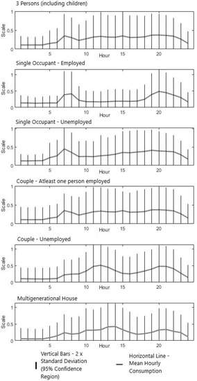
Figure 2.
Possibility curves for considered household types showing average loading and possible values in a 95% confidence interval.
2.7. Distributed Generation
The weather data for Berlin for the year 2014 shows the following trends:
Using this weather data mentioned in Table 2, solar production for an average day can be estimated from a normal distribution. This is used as data for solar panel production at different hours of the day, as shown in Figure 3.
Table 2.
Solar irradiation data [24].
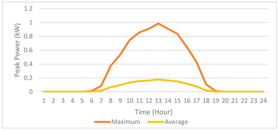
Figure 3.
Solar production data.
2.8. EV Implementation
Structurally, EVs are interfaces between mobile energy storage via batteries, through power electronics in both the charge controller (dc-dc converter), as well as through the electricity supply cabling required to output from the battery to the required powertrain. An EV charger provides carefully regulated DC voltage supply to the battery for charging the car. For low-voltage networks, both switch-mode power supply (SMPS) charging, also called slow charging, and typical are considered. Most EVs have the ability to charge from both. The model of a typical charging circuit is summarized in Figure 4.

Figure 4.
EV charging structure overview [26].
The electromagnetic interference filter removes high frequency noise from the input supply, which is converted to DC from AC and supplied to the battery for charging. For the purpose of this study, the EVs are assumed to be the commonly known Tesla Model S. This vehicle has a common range of between 250 and 350 miles per full charge of its 60 KWh battery pack. For this simulation, the cars are assumed to charge from a DC charging station supplying constant 7 kW instantaneous power. Current versus the charging characteristics of the Tesla Model S are summarized in Figure 5.
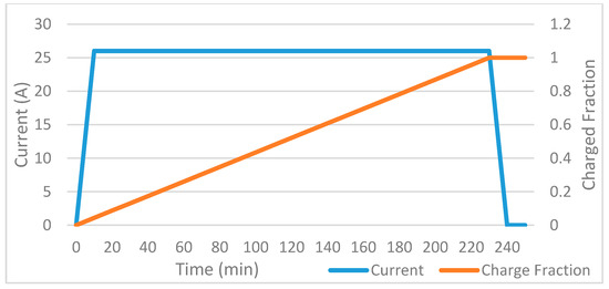
Figure 5.
Current vs. battery charging fraction for Tesla Model S measured by authors.
2.9. EV Penetration
It is expected that higher penetration of EVs in a population will lead to higher overall load profiles over the grid. These will be distributed nonlinearly, independent of the electricity consumption of the modelled houses. For this study, scenarios highlighted in Table 3 are compared.
Table 3.
Penetration scenarios.
2.10. EV Charging Distribution
In order to understand the likelihood of charging at a particular time and day, data from a study in southern Germany based on German and French EV adopters indicates that the likelihood of charging on a particular day varies slightly and can be assumed to be constant [13]. The variation in likelihood to plug in is significant. Figure 6 shows the variation between the number of vehicles charging at any given hour. The data shows a peak at hour 14 and another at hour 18, which is consistent with other such studies done in the past [13].

Figure 6.
EV State of Charge Estimation [13].
The amount of energy required every time an EV is plugged in is dependent on its state-of-charge (SOC) at the moment of plug in. Different users have been shown to react differently to their vehicle’s SOC, and the likelihood of plugging in therefore shows significant variation. An equivalent study on the use of EVs showed that the mean energy required per instance of charging is 6.31 kWh, with a standard deviation of 8.12 kWh [13,27]. This results in a normal distribution, as shown in Figure 7a.
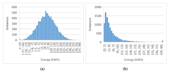
Figure 7.
(a) Normal distribution energy requirement per charging instance, (b) Lognormal distribution energy requirement per charging instance.
Upon conversion of these normal distribution parameters to logarithmic normal distribution, the distribution shows a mean of 1.3537 and a standard deviation of 0.9883. Figure 7b shows the related lognormal distribution sampling, showing the likely energy requirements per instance of charging for EVs.
Using these distributions and a neural network is trained that represents line loading percentage (based on instantaneous current as a fraction of individual cable rated current), voltage drops and line losses (based on instantaneous current and cable resistivity) individually. This neural network represents the grid accurately with a mean square error (MSE) less than 5% of the expected value in every scenario. Some intentional white noise is allowed in the network so as to allow variations in solar irradiance due to cloud cover or other imperfections. The algorithm for the entire simulation is summarized in Figure 8.
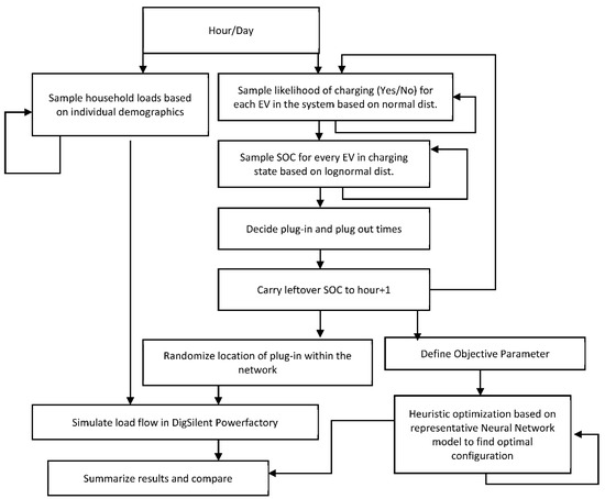
Figure 8.
Overall Monte Carlo simulation methodology. For each hour, the simulation is repeated 107 times to achieve a representative normal distribution.
3. Optimization Formulation
3.1. Optimization of Charging Locations Based on Minimizing Peak Line Loading
The overall objective function for minimizing the peak loading percentage across all lines as a product of varying the spatial distribution of charging EVs in the network is defined as follows,
where x1 refers to the set of values representing the number of EV charging in the network at a given time t on all of the possible charge locations. While, is the current flowing through line n and is the rated current of that individual line. The term refers to the current in line n observed in the lines as a result of household loads, in the absence of any EV load. This is time-dependent and originates from a separate set of probability distributions, hence dependent on the independently sampled variable x2, signifying the set of household load values with dimensions (1,11). Two scenarios are calculated for this redistribution optimization:
- No limit on the number of EVs charging at every node (ideal)
- No node can charge a number of EVs greater than 25% of the total vehicles charging in that grid at any given instant.
3.2. Optimization of Charging Locations Based on Minimizing Peak Voltage Drops Loading
The objective function for minimizing observed voltage drops at any given node in the network can be expressed as a maximization function of the minimum value in a set of voltages, observed at every terminal of the network. This can be determined as follows,
where is the minimum value from a set of voltage differences observed between the rated voltage and the observed line to line voltage at every node in the network. The observed line-to-line voltage is calculated using the equation(X), and is dependent on the sets x1 and x2, where x1 refers to the set of values representing the number of EV charging in the network at a given time t on all of the possible charge locations. Similarly, x2 is the set of independently sampled household loads with dimensions (1,11). Two scenarios are calculated for this redistribution optimization:
- No limit on the number of EVs charging at every node (ideal).
- No node can charge a number of EVs greater than 25% of the total vehicles charging in that grid at any given instant.
3.3. Optimization of Charging Locations Based on Minimizing Total Line Losses
For the purpose of this optimization, total loss in the system is the sum of all individual thermal losses in the lines, as a result of their inherent line impedance characteristics interacting with an increase in the current flowing in each line due to an additional EV charging at a particular location. This is calculated as the sum of the product of the square of the current flowing in a line n, and its equivalent impedance Z:
In this optimization equation, the variable x2 representing a set of values of household loads at a time t is independently sampled from a random distribution, and the sum of the set of values representing the number of EVs at every node is x1.
4. Simulation Results
Figure 9 shows a simplified layout of the grid with terminals 1–11 and lines 1–11 labelled.
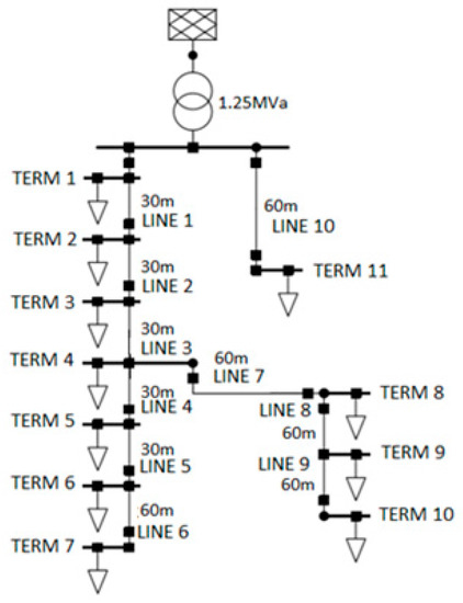
Figure 9.
Simplified grid layout line diagram—single-phase equivalent.
4.1. Charging Location Likelihood
The costs associated with increasing EV penetration, when run in tandem with peak theoretical household loads, results in different preferences for where the EVs should be charged and are summarized in Figure 10.
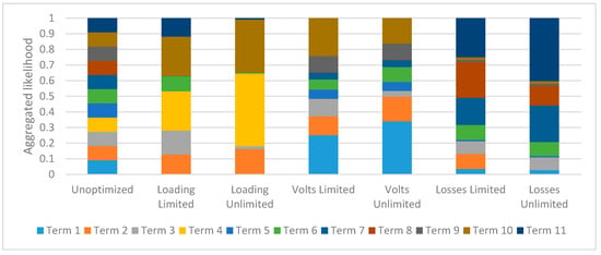
Figure 10.
Aggregated likelihood of new EV being plugged into a terminal when optimized for associated cost reduction.
4.2. Results—Optimization of Charging Locations Based on Minimizing Peak Voltage Drops Loading
Optimizing for a reduction in peak lineloading percentage results in lowering of line loads by 30 percent of their individual rated capacities in lines 1, 2 and 5, as shown in Figure 11. In all observed lines, adjusting the vehicle configuration according to the peak load results in the added increase for every 20 new EVs being kept almost negligible, as opposed to the nonlinear increase observed in the unoptimized case.
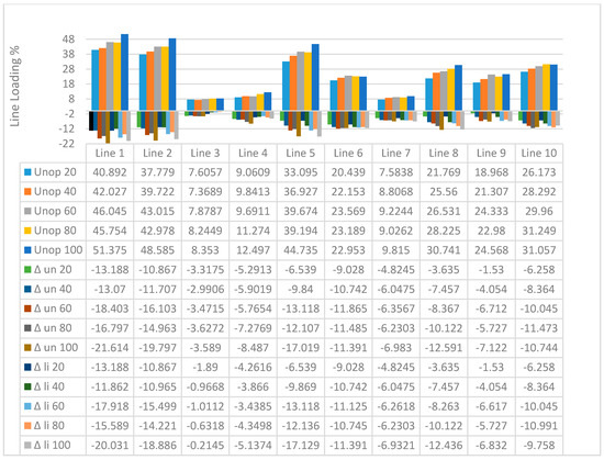
Figure 11.
Worst case line loading %–Unop (20–100): unoptimized with 20–100 EVs in the system; ∆ un (20–100) showing the change in loading percentages when optimized with no limit on the configuration configuration for between 20–100 EVs and ∆ li (20–100) showing the results optimized for minimizing peak line loading across all lines with no limit on configuration for between 20–100 EVs.
As can be seen in Figure 11, plugging in EVs in an optimized manner can result in maximum cable loading value being lowered by between 13% and 21% in line 1. Line 1 is the most significantly impacted due to increased EV penetration as it is the thoroughfare cable to other charging locations below. It is also observed that increasing number of EVs in the network allows for greater cable loading percentage shavings. This behavior can be attributed to more current being drawn by the larger magnitude of plugged in loads, which can then be lowered via optimizaiton. Forcing vehicles not to aggregate on a few terminals can lower the cable loading shavings to 11% but also encourages diversity in plug-in locations. Here, it is important to note that the number of simulations for every result is 107 and the shown values are the worst observed values across individual cables and nodes, not uniform scenarios. Figure 12 shows that the approach results in lower average loading percentage observed, and incremental increases in EV penetration also result in lower increases in average cable loading as a result.
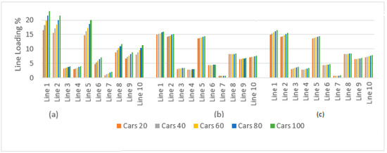
Figure 12.
Average observed line loading—(a) unoptimized versus, (b) optimized for minimizing peak line loading across all lines per vehicle with no limit on configuration, and (c) optimized for minimizing peak line loading across all lines per vehicle with no charging station having more than 25% of the vehicles charging at that hour.
By lowering the peak line loading observed in the simulation, the average line loading in cables 1, 2 and 5 also show lower values. The difference in average values is about 6%. This is seen across the other cables to a lesser extent. Cable 3 and 4 show no major decrease. Furthermore, the decrease in average loading caused by the addition of every 20 vehicles is reduced across all cables. In cable 8, this is reduced to an almost negligible increase. The difference in average loading observed between the unlimited optimization case, and when there is a limit on the configuration is negligible as well, showing no greater harm in not allowing the overall optimal situation.
4.3. Results—Optimization of Charging Locations Based on Minimizing Peak Voltage Drops Loading
In the unoptimized scenario, with 7 kW chargers, the peak load for 100 cars can lower the voltage by up to 6 volts across terminals 8, 9, 10, and 11. Optimizing for maximizing the minimum observed voltage shows an improvement in all terminals except terminal 4, which remains almost the same. Furthermore, when the configuration is limited to allow for only 25% of the total number of cars charging at that instant to charge at any one location, the performance is reduced in terminals 9 and 10 the most. In this optimization scheme, it is evident that the potential of redistributing electric vehicle charging configurations can yield significant improvements. It is also pertinent to note that in the available dataset, the times for peak EV charging and peak distributed solar production overlap, allowing peak load to be offset locally as well. As can be seen in Figure 13, plugging in EVs in an optimized manner can result in a reduction in maximum observed voltage drops across almost all nodes. Terminals 8 and 11 show increases in observed voltage levels by 7 V. This significantly reduces the problem of overloading causes high values of voltage drops due to high EV penetrations, as shown in Figure 13 and Figure 14.
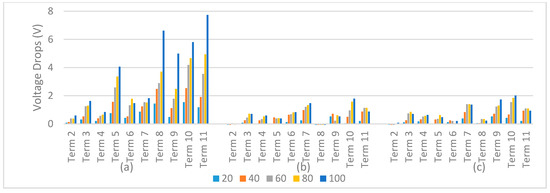
Figure 13.
Worst case voltage drops (line to ground) observed—(a) unoptimized versus, (b) optimized for minimizing peak voltage drops across all cables per vehicle with no limit on configuration, (c) optimized for minimizing peak voltage drops across all cables per vehicle with with no charging station having more than 25% of the vehicles charging at that hour.
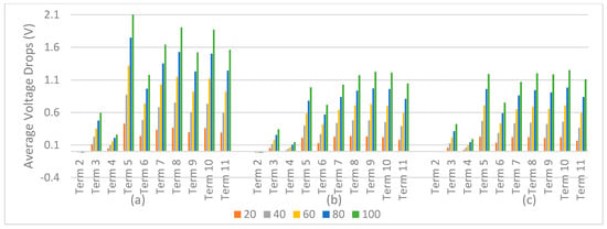
Figure 14.
Average case voltage level observed—(a) unoptimized versus, (b) optimized for minimizing peak voltage drops across all cables per vehicle with no limit on configuration, (c) optimized for minimizing peak voltage drops across all cables per vehicle with with no charging station having more than 25% of the vehicles charging at that hour.
4.4. Optimization of Charging Locations Based on Minimizing Total Line Losses in the Network
Optimization for reducing the sum of peak line losses at any given instant results in negligible benefits. In the worst case, line losses in individual cables are reduced between 2 and 5 watts. The total reduction in line losses is from 21 W instantaneous to 7 W in the worst case scenario as shown in Figure 15 and Figure 16. In the best-case scenario, cable losses are up to 1.5 W per cable. Extrapolating the worst case line losses to the entire year results in savings of approximately 173 units of energy, roughly equal to a cost savings of €25 annually at €0.20 per unit. This is an insignificant amount of savings that does not justify further work in optimization of electric vehicle charging configurations across densely packed low voltage networks. It is potentially important in networks with higher voltage levels and longer cable lengths. On average, Figure 17 shows insignificant savings across the network.
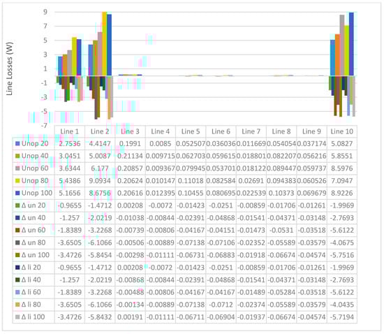
Figure 15.
Worst case line losses observed (W): Unop (20–100): unoptimized with 20–100 EVs in the system; ∆ un (20–100) showing the change in line losses across individual cables when optimized with no limit on the configuration configuration for between 20–100 EVs and ∆ li (20–100) showing the results optimized for minimizing line losses across all lines with no limit on configuration for between 20–100 EVs.
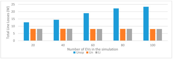
Figure 16.
Worst case total line losses (W) Unop—Unoptimized; Un—Unlimited configuration optimization; Li—Optimization with no node connected to more than 25% of the vehicles charging at that hour.
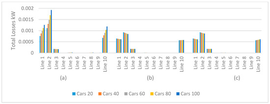
Figure 17.
Average line losses observed—(a) unoptimized versus, (b) optimized for minimizing total (sum) of line losses in the entire across all cables with no limit on confiuguration versus, (c) across all cables per vehicle with with no charging station having more than 25% of the vehicles charging at that hour.
5. Discussion
The simulation of electrical vehicle charging behavior, according to the associated probabilities shows equal propensity for charging at any of the available terminals, due to the inherent randomness. In the loading-unlimited case, the optimization prefers to connect to terminal 4 because lines 1, 2 and 3 are the have the largest diameter (240 mm) and show lower peak loading percentage and are not considered the choke point. Line 4 onwards have smaller diameters and longer lengths, so an increase in current flowing will increase the loading percentage greatly, due to lower rated current. Therefore, the optimization is avoiding placing the load in those locations, which would increase peak percentage loading in these cables. This is followed by terminal 2 for the same reason. For cars it cannot accommodate here, it is placing them at terminal 10, this is because household (not EV) load in terminals 5, 6 and 7 is higher than in terminals 8, 9 and 10 which means placing EVs in this string leads to less peak loading percentage in the cables.
In the voltage unlimited optimization case, it is placing most EVs at terminal 1, which is connected to the terminal directly with no voltage drop due to cable losses. This results in the lowest peak voltage drop. Terminal 2 is the closest and shows the same trend (lowest voltage drop due to current in only 1 cable with 240mm diameter). The other combination is distributed between terminals 3 to 10. While cables 4, 5 and 6 are shorter, they have higher peak household load, and terminals 8, 9 and 10 are further away but with less load. These are optimization results and depend on the time of the day, the type of household load at that time and the number of EVs needing to charge.
For line losses, the problem is optimized differently. The model prefers to place EVs at terminal 11, because that string is connected by only one cable, leading to the lowest sum of line losses. It also completely avoids terminal 9 and 10, which are the furthest from the grid connection, and thus, result in the highest sum of loads observed. However, the total saved power loss is approximately 17 watts across the network. This number is insignificant compared to the voltage drop and line loading scenarios. It is evident that in similar LV networks, power loss values will not warrant significant change in charging behaviour. For all the limited loading scenarios, the optimization model(s) result in similar trends but show hard cuts where no single terminal is allowed to charge more than 25% of the total EVs charging at that hour. This causes the likelihood to appear more distributed.
It is difficult to compare the results of the three different optimization results presented. This is due to the differences between the optimization objective function itself. Comparing the percentage line loading to voltage drops is not feasible, due to the propensity of voltage drops to fluctuate in single digits, whereas cable loading shows significantly greater possible ranges. Furthermore, line loading percentage is a relatively easy problem to solve by increasing the number of parallel conductors across lines 1, 2 and 5. Voltage drops are unlikely to be resolved by cable upgrades and would require reactive power injection at specific locations, a technique whose effectiveness at the 0.4 kV level requires further inquiry to recommend. Line losses are insignificant in the low voltage network and do not warrant heuristic optimization. In comparison to literature, optimizing EV charging locations within one feeder as opposed to optimizing the availability of charging spots over one day allows an easier solution that does not involve significant changes in user behavior. This approach can be used to come up with a location dependent price surcharge factor later on.
6. Conclusions
The simulation results suggest that EVs will add a significant amount of loading and voltage drops when added randomly to low-voltage networks over time. This can be mitigated by exploiting the inherent structure of any LV network, where differences in cable sizes and household load profiles can be used to rearrange vehicles, or limit access of some vehicles at some locations, in order to reduce overall negative overloading effects in the network. This can be achieved through optimizing of a reduction in peak loading and voltage drops and voltage drops. In smaller LV networks with less cable diameters, particularly in developing areas, this methodology could be essential to allow for the addition of fast chargers in LV networks, in order to enable the introduction of EVs without having to install thicker cables, and install other costly equipment upgrades to account for the increased demand.
In the next phase, the authors propose development of a spatial pricing system to account for differences in system overloading based on vehicle charging configuration. This pricing should be used in conjunction with existing temporal pricing models to better reflect the loading caused in the cost of electricity available to EVs. The optimization model would unify the optimization models discussed in this study by way of quantifying their effects and introducing surge pricing at smart meters within one feeder. Further simulation should also look at the possibility of changing the car charging algorithm from a car-by-car basis, as currently presented, to an overall configuration, which might further improve optimization results as compared to the current model.
Author Contributions
Literature search, S.H.; data curation and creation, S.H.; methodology design, S.H. and P.S.; data validation, S.H.; simulation and results consolidation, S.H.; Supervision, P.S.; revisions and proofreading, P.S. Both authors have read and agreed to the published version of the manuscript.
Funding
This research was made possible by the funding provided by the Boysen–TU Dresden ResearchTraining Group.
Conflicts of Interest
The authors declare no conflict of interest.
References
- Strunz, K.; Abbasi, E.; Abbey, C.; Andrieu, C.; Gao, F.; Gaunt, T.; Iravani, R. Benchmark systems for network integration of renewable and distributed energy resources. Cigre Task Force C 2009, 6, 78. [Google Scholar]
- Hu, J.; Morais, H.; Sousa, T.; Lind, M. Electric vehicle fleet management in smart grids: A review of services, optimization and control aspects. Renew. Sustain. Energy Rev. 2016, 56, 1207–1226. [Google Scholar] [CrossRef]
- Widén, J.; Lundh, M.; Vassileva, I.; Dahlquist, E.; Ellegård, K.; Wäckelgård, E. Constructing load profiles for household electricity and hot water from time-use data—Modelling approach and validation. Energy Build. 2009, 41, 753–768. [Google Scholar] [CrossRef]
- Al-Alawi, B.M.; Bradley, T.H. Review of hybrid, plug-in hybrid, and electric vehicle market modeling Studies. Renew. Sustain. Energy Rev. 2013, 21, 190–203. [Google Scholar] [CrossRef]
- Hawkins, T.R.; Singh, B.; Majeau-Bettez, G.; Strømman, A.H. Comparative Environmental Life Cycle Assessment of Conventional and Electric Vehicles. J. Ind. Ecol. 2012, 17, 53–64. [Google Scholar] [CrossRef]
- Sioshansi, R.; Denholm, P. Emissions Impacts and Benefits of Plug-In Hybrid Electric Vehicles and Vehicle-to-Grid Services. Environ. Sci. Technol. 2009, 43, 1199–1204. [Google Scholar] [CrossRef]
- Green, R.C.; Wang, L.; Alam, M. The impact of plug-in hybrid electric vehicles on distribution networks: A review and outlook. Renew. Sustain. Energy Rev. 2011, 15, 544–553. [Google Scholar] [CrossRef]
- Sachan, S.; Adnan, N.; Amini, M.H. Stochastic charging of electric vehicles in smart power distribution grids. Sustain. Cities Soc. 2018, 40, 91–100. [Google Scholar] [CrossRef]
- Shi, Y.; Tuan, H.D.; Savkin, A.V.; Duong, T.Q.; Poor, H.V. Model Predictive Control for Smart Grids With Multiple Electric-Vehicle Charging Stations. IEEE Trans. Smart Grid 2018, 10, 2127–2136. [Google Scholar] [CrossRef]
- Alonso, M.; Amaris, H.; Germain, J.G.; Galan, J.M. Optimal Charging Scheduling of Electric Vehicles in Smart Grids by Heuristic Algorithms. Energies 2014, 7, 2449–2475. [Google Scholar] [CrossRef]
- Fäßler, B.; Schuler, M.; Preißinger, M.; Kepplinger, P. Battery Storage Systems as Grid-Balancing Measure in Low-Voltage Distribution Grids with Distributed Generation. Energies 2017, 10, 2161. [Google Scholar] [CrossRef]
- Ensslen, A.; Will, C.; Jochem, P. Will Simulating Electric Vehicle Diffusion and Charging Activities in France and Germany. World Electr. Veh. J. 2019, 10, 73. [Google Scholar] [CrossRef]
- Schäuble, J.; Kaschub, T.; Ensslen, A.; Jochem, P.; Fichtner, W. Generating electric vehicle load profiles from empirical data of three EV fleets in Southwest Germany. J. Clean. Prod. 2017, 150, 253–266. [Google Scholar] [CrossRef]
- Sachan, S.; Deb, S.; Singh, S. Different charging infrastructures along with smart charging strategies for electric vehicles. Sustain. Cities Soc. 2020, 60, 102238. [Google Scholar] [CrossRef]
- Bradley, T.H.; Frank, A.A. Design, demonstrations and sustainability impact assessments for plug-in hybrid electric vehicles. Renew. Sustain. Energy Rev. 2009, 13, 115–128. [Google Scholar] [CrossRef]
- Gnann, T.; Stephens, T.S.; Lin, Z.; Plötz, P.; Liu, C.; Brokate, J. What drives the market for plug-in electric vehicles? A review of international PEV market diffusion models. Renew. Sustain. Energy Rev. 2018, 93, 158–164. [Google Scholar] [CrossRef]
- Uddin, M.; Romlie, M.; Abdullah, M.F.; Halim, S.A.; Abu Bakar, A.H.; Kwang, T.C. A review on peak load shaving strategies. Renew. Sustain. Energy Rev. 2018, 82, 3323–3332. [Google Scholar] [CrossRef]
- Liao, F.; Molin, E.; Van Wee, B. Consumer preferences for electric vehicles: A literature review. Transp. Rev. 2016, 37, 252–275. [Google Scholar] [CrossRef]
- Fasugba, M.A.; Krein, P.T. Gaining vehicle-to-grid benefits with unidirectional electric and plug-in hybrid vehicle chargers. In Proceedings of the 2011 IEEE Vehicle Power and Propulsion Conference, Chicago, IL, USA, 6–9 September 2011; pp. 1–6. [Google Scholar]
- Haider, S.; Schegner, P. Data for Heuristic Optimization of Electric Vehicles’ Charging Configuration Based on Loading Parameters. Data 2020, 5, 102. [Google Scholar] [CrossRef]
- Statistisches Bundesamt. Statistisches Bundesamt wissen.nutzen. 2019. Available online: https://www.destatis.de/EN/Themes/Society-Environment/Population/_node.html (accessed on 12 January 2020).
- Pflugradt, N.; Muntwyler, U. Synthesizing residential load profiles using behavior simulation. Energy Procedia 2017, 122, 655–660. [Google Scholar] [CrossRef]
- Zhao, H.; Yan, X.; Ren, H. Quantifying flexibility of residential electric vehicle charging loads using non-intrusive load extracting algorithm in demand response. Sustain. Cities Soc. 2019, 50, 101664. [Google Scholar] [CrossRef]
- NASA. POWER Project, NASA Langley Research Center (LaRC) POWER Project. 2019. Available online: https://power.larc.nasa.gov/ (accessed on 20 January 2020).
- Siano, D.B. The log-normal distribution function. J. Chem. Educ. 1972, 49. [Google Scholar] [CrossRef]
- Gautam, D.S.; Musavi, F.; Edington, M.; Eberle, W.; Dunford, W.G. An Automotive Onboard 3.3-kW Battery Charger for PHEV Application. IEEE Trans. Veh. Technol. 2012, 61, 3466–3474. [Google Scholar] [CrossRef]
- Ensslen, A.; Jochem, P.; Schäuble, J.; Babrowski, S.; Fichtner, W. User Acceptance of Electric Vehicles in the French-German Transnational Context: Results out of the french-german fleet test ‘cross-border mobility for electric vehicles’ (CROME). In Proceedings of the 13th WCTR, Rio de Janeiro, Brazil, 15–18 July 2013. [Google Scholar]


Publisher’s Note: MDPI stays neutral with regard to jurisdictional claims in published maps and institutional affiliations. |
© 2020 by the authors. Licensee MDPI, Basel, Switzerland. This article is an open access article distributed under the terms and conditions of the Creative Commons Attribution (CC BY) license (http://creativecommons.org/licenses/by/4.0/).