Article

A Simulation Approach for Optimising Energy-Efficient Driving Speed Profiles in Metro Lines †

1
Department of Engineering, University of Sannio, Piazza Roma 21, 82100 Benevento, Italy
2
Department of Civil, Architectural and Environmental Engineering, Federico II University of Naples, Via Claudio 21, 80125 Naples, Italy
3
Rete Ferroviaria Italiana S.P.A. (RFI), Via Marsala 75, 00185 Rome, Italy
*
Author to whom correspondence should be addressed.
This paper is an extended version of our paper published in 20th IEEE International Conference on Environment and Electrical Engineering (IEEE EEEIC 2020) and 4th Industrial and Commercial Power Systems Europe (I&CPS 2020), Madrid, Spain, 9–12 June 2020; pp. 886–891.
Energies 2020, 13(22), 6038; https://doi.org/10.3390/en13226038
Submission received: 26 October 2020 / Revised: 16 November 2020 / Accepted: 17 November 2020 / Published: 19 November 2020

Abstract

:
We propose a model for optimising driving speed profiles on metro lines to reduce traction energy consumption. The model optimises the cruising speed to be maintained on each section between two stations; the functions that link the cruising speed to the travel time on the section and the corresponding energy consumption are built using microscopic railway simulation software. In addition to formulating an optimisation model and its resolution through a gradient algorithm, the problem is also solved by using a simulation model and the corresponding optimisation module, with which stochastic factors may be included in the problem. The results are promising and show that traction energy savings of over 25% compared to non-optimised operations may be achieved.

1. Introduction

Energy savings, and hence, the reduction in greenhouse gas emissions and air pollutants are major challenges for planners and transport operators. The importance of this theme is underlined in European documents [1,2]. Transport activities contribute significantly to energy consumption and harmful emissions: For example, in Europe, 31% of the total energy consumed is accounted for by the transport sector [3]. From this perspective, the White Paper [4] disseminated by the European Union identifies several actions that need to be implemented to reduce emissions.
Although road transport can be identified as the main culprit, rail systems have also been examined from this angle [5]. Indeed, all components of the transport sector can contribute to the reduction in energy consumption. Besides, the rising costs and the increased demand for electricity (especially in developing countries) make it important to reduce energy consumption in the rail sector as well.
Among the possible strategies that can be used to reduce rail energy consumption (low consumption engines, energy recovery systems, etc.), energy-efficient driving, or eco-driving, is one of the most promising [6,7,8]. This lies in the following strengths: (1) It can be adopted even with current trains (rolling stock need not be changed); (2) it requires low investments (the cost of the information system needed to implement the strategy is very low compared to the procurement cost of the train); (3) the time needed for its implementation can be low because the system does not require any intervention on the railway infrastructure or rolling stock.
It is necessary to distinguish energy-efficient driving applied to automatic train operation (ATO), where the whole driving speed profile may be designed, from the same strategy applied to human-driven trains, where only some movement parameters can be effectively controlled and optimised. In this document, we focus on energy-efficient driving applied to human-driven trains, which could also be implemented on lines currently in operation, with limited monetary investments.
Energy efficiency has been extensively studied mainly from a technological point of view. Indeed, technology is constantly evolving, and urban rapid transit systems are now managed with a high degree of automation, improving reliability and safety in rail traffic control [9]; such automation can introduce energy-efficient driving strategies [10]. Automatic train operation (ATO) systems have been widely managed, especially in urban and suburban contexts, by determining optimal speed profiles in terms of running time or energy expenditure [11]. Interesting results have been obtained by loading predefined speed profiles into the system so that, based on the departure time and the minimum running time required, the speed profile that best suits the requirements of the strategy is selected [12]. Other significant results on specific rail systems can be found in Reference [13] on the operation of freight trains, in Reference [14] on the planning of mass rapid transit systems and in Reference [15] on the signalling systems of moving blocks. Optimisation procedures for the definition of energy-efficient speed profiles have also been extensively studied. Some papers have addressed the topic by formulating an optimal control problem [16,17]. Other interesting results on the optimisation of speed profiles were obtained in References [18,19,20,21,22,23,24,25,26,27,28].
New information technologies, together with the continuous evolution of optimisation algorithms and the opportunity offered by new ICT, have recently pushed many studies to implement different solutions that lead to very interesting results and prospects [29,30,31,32,33]. Concerning train/driver interaction, in Reference [34] the author proposed energy-optimal train control, based on a two-level algorithm that leads to the energy-optimal regime sequence with the minimum number of regime changes, to be easily followed by the driver.
Timetable reprogramming procedures and algorithms are often used jointly with eco-driving strategies [35,36]; Especially to reallocate train starts or acceleration regimes to coincide with the braking regime of other trains within the same powered section to optimise the use of recovered energy that would otherwise be dissipated in heating resistors [37]. Further, in Reference [38] the authors proposed an optimisation procedure which first optimises the speed profiles of each train and then increases the receptivity of the network to achieve a compromise between efficient speed profiles and regenerated energy maximisation. In Reference [39], the authors proposed several efficient on-board recovery systems that allow train operations to be independent of other train regimes. In References [40,41], the authors adopted a microscopic approach to analyse the effects of different driving strategies in terms of energy consumption.
This paper extends the authors’ research into driving speed profile optimisation [42], proposed at the 20th IEEE International Conference on Environment and Electrical Engineering (IEEE EEEIC 2020) and 4th Industrial and Commercial Power Systems Europe (I&CPS 2020). The above work was enhanced by extending the description of the problem and the case study, which were tackled by using a simulation-based methodology. This innovation also allowed stochastic aspects to be considered, neglected with the resolution of the optimisation problem. Use was made, in particular, of the general-purpose simulation software Arena in which the case study was implemented. Therefore, the final results were also extended.
However, in contrast to the existing literature where the problem has been studied almost exclusively for suburban and regional railways, this work focuses on the case of urban metro lines, where the lengths of the sections (i.e., the distances between two successive stations) are usually less than 2 km. In this case, as will be clearer in the next section, the strategies of running management are significantly different from the case of suburban and regional railways.
The paper is organised as follows: Section 2 examines the problem, highlighting the differences with the cases already covered in the literature; the mathematical formulation of the optimisation model is reported in Section 3; Section 4 illustrates the case study; Section 5 summarises the numerical results; finally, Section 6 concludes the work and outlines research prospects.

2. Problem Description

Energy-efficient driving on rail systems aims to save traction energy by optimising the running profile on a section between two stations or along a route. In this case, we operate only on the train speed profiles along the section. As mentioned in Section 1 and shown in the literature, good results can be achieved both by fully automatic train control and by acting on driving behaviour, providing the driver with the necessary information in real-time to get as close as possible to the optimal driving pattern.
For suburban and regional services, where stations are usually more than 2 km apart, it is assumed that the scheduled timetable, and hence, the departure time of each train from each station are known. Scheduled timetables are designed so that the departure time from a station is equal to the departure time from the previous station plus the minimum running time, mrt, between stations, plus the dwell time (necessary for passengers to board and alight), dt, plus the reserve time, rt (see Figure 1). The reserve time is provided to recover a possible delay of a train so that the departure time from the next station is respected (if the delay is less than the scheduled reserve time). Details on the definition of dwell time can be found in Reference [43]; similarly, the reserve time calculation is shown in Reference [44].
If a train departs late, the driving style must ensure the minimum running time, i.e., maximum acceleration, maximum cruising speed and maximum deceleration (compatible with comfort standards, speed limits and available power). This driving style is also known as time-optimal (or all-out) and is the driving style with the maximum energy consumption; in Figure 2 an all-out driving profile is schematically shown, where tacc is the duration of the acceleration phase, tcru is the duration of the cruising phase, tdec is the duration of the deceleration phase, and spmax is the maximum travel speed.
By contrast, if the train is on time, the reserve time can be used to optimise the driving style to minimise energy consumption. Indeed, reducing the cruising speed and/or introducing a coasting phase (the propulsion system is turned off and the train runs using kinetic energy, reducing its speed) allows energy consumption to be reduced. In Figure 3, two possible energy-saving driving styles are reported: (a) With a coasting phase; (b) without a coasting phase. In Figure 3, besides the already defined terms, tcoa is the duration of the coasting phase, and spcru is the (optimised) cruising speed.
Compared to the case of regional or suburban services, metro lines have two different characteristics that require us to formulate the problem differently. First of all, reserve time is not available at each section because the service is not schedule-based but frequency-based: The operator will try to respect only the departure times from the terminals, to maintain the expected headway, but no departure time is defined at each station. Consequently, the reserve time is provided only at terminals (see Figure 4). The second difference concerns the substantial impossibility of operating an energy-saving driving style with coasting, given the short length of the sections; only with a fully automated train would it be possible. In the next section, an optimisation model based only on speed optimisation is proposed.

3. Optimisation Model

Although the problem of eco-driving on suburban and regional railway lines has been widely addressed in the literature [22,23,24,25,26,27], to our best knowledge there has been no specific coverage of metro lines, except for the paper that we are now extending [42].
Herein we assume that, as usually happens, the metro line is frequency-based, reserve time is available only at both terminals, and that the decision variables are only the cruising speeds which the driver must not exceed. The problem, therefore, is to optimise the cruising speeds on the different sections of the line to reduce energy consumption while respecting the departure times from the terminals.
Although not covered in this work, the practical application of the results obtained is possible by training staff and equipping the driver’s cab with an intelligent dashboard that communicates with the driver or, if necessary, automatically limits the maximum speed on the section. This speed must, of course, be lower than the maximum technically possible depending on the elevation and curvature characteristics of the track. If the train is late, the dashboard will communicate the maximum possible cruising speed (all-out); if, on the other hand, the train is on time, compared to the expected values, the dashboard will communicate the optimal speed obtained with the procedure.
The problem can be solved by formulating a non-linear constrained optimisation model, where the function to optimise (minimise in this case) is the total traction energy used by the train running on a metro line and the constraints concern the possible speed ranges on each section and the respect of departure times from the terminals. The proposed optimisation model is as follows:
sp^ = Arg sp min ET(sp) = Arg sp min Σi EiT(spi)
s.t.
spminispispmaxi        ∀ i
Σiot ti(spi) ≤ Σiot ti(spmaxi) + RTot
Σirt ti(spi) ≤ Σirt ti(spmaxi) + RTrt
where
  • sp is the decision variables vector, whose generic element is term spi;
  • spi is the cruising speed (m/s) that the train must not exceed when running on section i;
  • sp^ is the optimal value for sp;
  • ET(.) is the total traction energy used by a convoy on the metro line for each outward plus return trip;
  • EiT(.) is the traction energy used by a metro train on section i;
  • spmini is the minimum value of spi on section i (m/s);
  • spmaxi is the maximum value of spi on section i (m/s), which depends on the features of the railway track and of rolling stock: Such values are those corresponding to a non-optimised (all-out driving style) solution;
  • ti(.) is the expected running time (s) of each section i, which depends on spi;
  • ot represents the set of rail sections belonging to a direction of the metro line (for instance, from terminal A to terminal B);
  • rt represents the set of rail sections belonging to the other direction of the metro line (for instance, from terminal B to terminal A);
  • RTot is the reserve time available at terminal B;
  • RTrt is the reserve time available at terminal A.
Note that ti(spmaxi) is the minimum running time on rail section i (all-out driving style), and in constraints (3) and (4) the dwell times are neglected. Indeed, they are the same in all driving styles and thus, if considered, they cancel each other out in the constraints.
Whatever the resolution method of the model (1–4), we need to know the functions that link traction power consumption and total travel time with the cruising speed value, respectively EiT(spi) and ti(spi). These functions cannot be generalised, but must be calibrated on each section, taking into account the performance of the rolling stock and the real curvature and elevation track profile. Therefore, we propose that these functions should be calibrated using a microscopic simulation model of railway motion, which can take into account the specific situation of each section and the rolling stock travelling on it. The definition of these functions is thus reported in the next section, where the case study is presented.

4. Case Study

The proposed method was applied to a real case, Line 1 of the Naples Metro. The city of Naples has just under one million inhabitants, is the capital of the region of Campania, and is the third-most populous city in Italy after Rome and Milan. Line 1 is a fundamental infrastructure for urban mobility and connects the northern part of the city with the historic centre and the central station, passing through the densely populated hillside districts. Figure 5 shows the layout of the line, which has 18 stations and 17 sections.
As underlined in the previous section, the functions that link traction energy consumption and travel times to cruising speeds have to be calibrated. To do so, a detailed model of the line was built using OpenTrack railway microsimulation software; Figure 6 shows the graphic representation of the supply model. To build a microscopic simulation model of a rail line, it is generally necessary to reproduce its features in terms of infrastructure, signalling and control systems, rolling stock, timetable and travel demand flows. However, in this specific case, given the fact that the goal is limited to capturing the relationship between speed values on the one hand and related travel times and energy consumption on the other, the modelling of infrastructure features (in terms of slope, curvature radii and tunnel sections) and rolling stock characteristics (in terms of the tractive effort curve) is required. Further, it is worth noting that the simulation model, given its calibration purposes, considers an isolated convoy, and therefore, circulation rules related to the spacing between two successive convoys, dictated by signalling and control systems, are neglected. By contrast, signalling and control issues governing trains entering and leaving stations were accurately modelled.
Once the model was built, several simulations were performed, considering different maximum cruising speeds, falling within a range between a minimum of 30 km/h and a maximum of 80 km/h, with steps of 2 km/h, for a total of 26 simulated scenarios. The upper limit (80 km/h) takes into account the maximum speed allowed on the fastest section of the line, while the lower limit (30 km/h) is set to avoid excessively long travel times. Clearly, on some sections the maximum value was reduced to take into account the actual maximum speed possible for safety reasons; on other sections, on the other hand, the convoy cannot reach the maximum speed (especially on some uphill sections). For each scenario (cruising speed) and each section, the simulation results were extracted, in terms of travel time and traction energy consumed. These data made it possible to calibrate the functions to be used in the optimisation model.
In Figure 7, some examples of the relationship between travel time and cruising speed are reported; the interpolating functions for each metro section are assumed quadratic:
ti(spi) = a0 + a1 spi + a2 spi2
In Figure 8, instead, some examples are reported of the relation between energy consumed and maximum speed resulting from the simulations; the interpolating functions, in this case, are assumed linear:
EiT(spi) = b0 + b1 spi
Table 1 and Table 2 report the values assumed by the coefficients for each section. Note that the values of the coefficient of determination are almost always very close to 1, and therefore, the calibrated functions accurately reflect the actual line.

5. Solution Approaches and Numerical Results

For solving the optimisation model (1–4), we propose two different approaches. The first is based on using a generalised reduced gradient (GRG) algorithm. In this case, the possibility of on-line delays is not considered in any way and the values obtained, thus, represent ideal ones. It is expected that it is not always possible to reach such values because, as stated above, the optimal cruising speed can be used on the section only if the train is not delayed. The second approach consists in implementing the line through a discrete simulation model, built, in our case, with Arena software [45] and Optquest for Arena [46], which is an optimisation module that can be used in Arena. It is thereby possible to include in the model some delay travel time functions on every section and simulate, should the delay of one train be such as to prevent the next train occupying the same section, the propagation of the delay to the following trains. The functions calibrated in Section 4 were used in both cases and the following assumptions, considering the real operation of the metro line, were considered: (i) Dwell times of 20 s at each station; (ii) a reserve time of 240 s at each terminal.

5.1. Results with the GRG Algorithm

The optimisation model (1–4) was implemented in Excel and solved with the GRG algorithm included in the Solver tool. In Table 3, we report the data before optimisation of cruising speeds; in this case, all speed profiles are those corresponding to the minimum running times (all-out). In Table 4, instead, the same data after optimisation are reported; note that the reserve times are entirely used. Indeed, the solution of the problem distributes the reserve time between the rail sections, optimising the maximum speed on each section. Total traction energy consumption decreases from 678.332 kWh to 505.668 kWh, amounting to a reduction of about 25%.
It should be pointed out that this reduction is the most that can be achieved, assuming that there are no delays to be made up along the line. Indeed, when a train has accumulated a delay, the following sections will have to be run assuming the highest value of the maximum speed along the sections until the delay is recovered. The real savings can be assessed based on the regularity of the line. Using the whole reserve time, the number of trains needed for the service is 11, which is the same as the case of all-out driving style. Of course, although the cycle time, which includes the recovery times, is the same, the travel times for users increase up to about 13% (depending on trip length).
Moreover, the optimisation model was also applied to several reserve times to assess how much energy could be saved by increasing the train cycle time, and hence, the time available to implement the energy-saving strategy. The reserve time was, therefore, increased up to 400 s, verifying whether an additional train would need to be put into operation. Table 5 summarises the results obtained.
These results show that energy consumption may be significantly reduced with appropriate management of metro trains. The energy-saving values, shown in Table 5 (varying from 25% to 30%), are the maximum obtainable (service perfectly regular). However, even if the actual savings were only one-third of the maximum, an 8–10% reduction in energy consumption can be achieved, with a significant benefit in the overall energy balance of a line.

5.2. Results with Arena and Optquest

The outward and return routes of line 1 were modelled with Arena software. A portion of the outward route (sections: Piscinola-Chiaiano, Chiaiano-Frullone) is reported in Figure 9. The modules used to construct the simulation model are as follows:
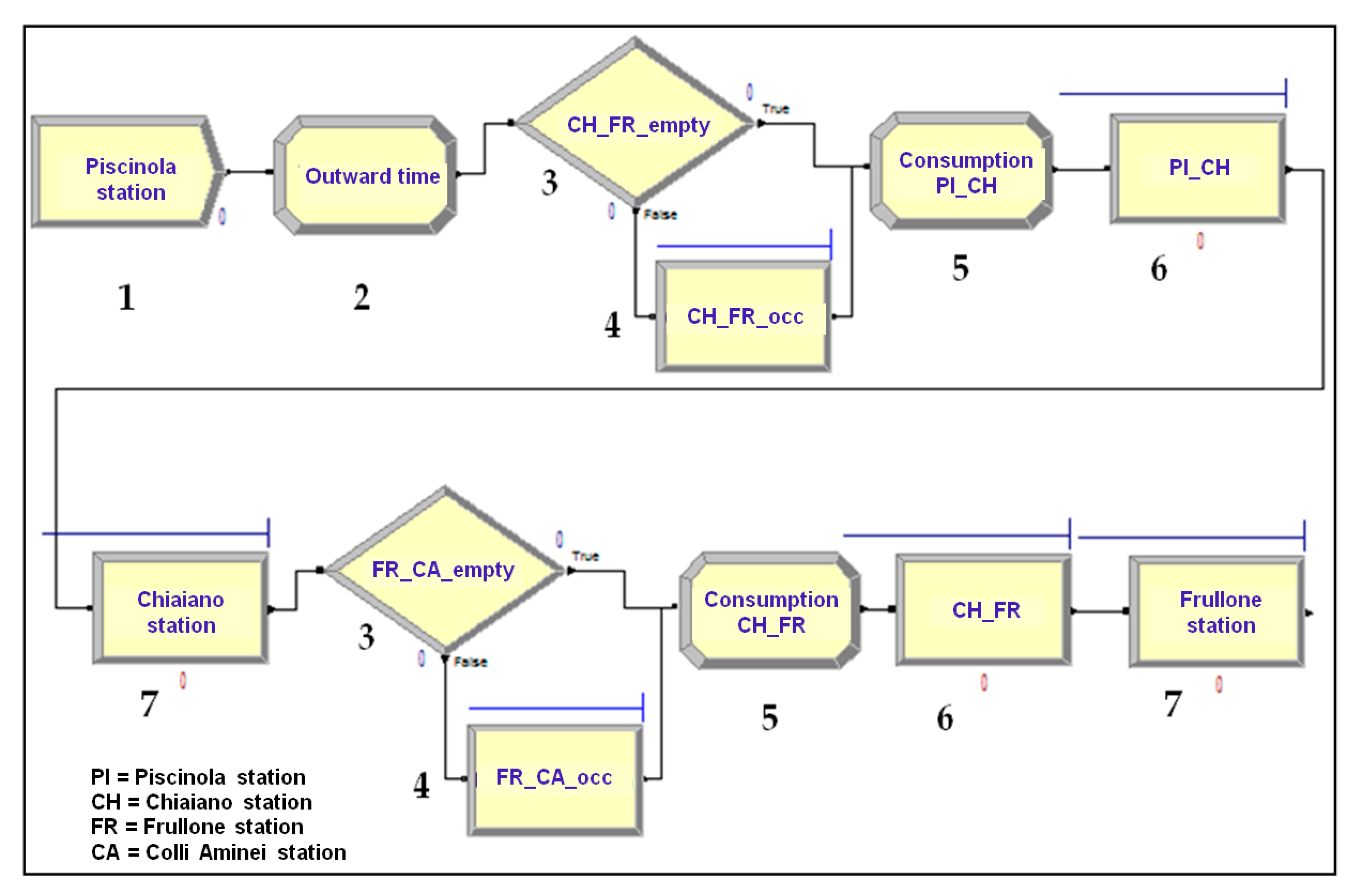
  • Create. This module represents the end of the line; it was set to generate a convoy every 480 s, which is the headway of the line.
  • Assign. This module is necessary to record the outward time of the convoy from the terminal to arrive at the other terminal (before arrival there is a Record module, not shown in the figure, which is used to record statistics on convoy journey times).
  • Decide. This module verifies the occupation of the sections and allows the train to enter the section (module 5) only if the next two sections are empty. Otherwise, the train will have to wait, and in the simulation model, it will be directed to module 4.
  • Hold. This module hosts the convoy until the next two sections are empty.
  • Assign. This second assign module is used to calculate the traction energy consumption variable on the section. This expression links travel times to consumption and is obtained, on each section, by combining Equation (5) with Equation (6) to obtain a relation between consumption and travel time.
  • Process. This module represents the resources, in terms of railway tracks, of the section. The capacity attributed to the module is equal to 1: Only one train can occupy the section at the same time. Moreover, a delay function is included, representing a negative exponential distribution of an average of 7.5% of the total travel time of the section.
  • Process. This second process module represents the presence of the train in the station. In this case, the time the train stays in the station is represented by a normal variable of mean 20 s and a standard deviation of 0.2.
This scheme is replicated for all sections. After the last section, two final modules are inserted: (a) a Record module to register the total outward time and an Assign module to represent the total consumption variable, equal to the sum of the consumption on each section; (b) a Dispose module representing the last station, where the convoy ends its run.
The simulation of the overall system was performed considering 18 h of operation and was repeated 100 times, since the problem has several stochastic aspects (delays on sections and dwell times at stations).
After simulating the outward and return operation of line 1, OptQuest software for Arena was used to optimise energy consumption. The decision variables (or control variables), in this case, are the travel times on each section, clearly as a function of cruising speed, while the objective function is overall consumption along the route. The constraints of the problem are the minimum and maximum travel time (depending on the maximum and minimum speed planned on each section) and the total travel time which cannot exceed the time in all-out conditions plus the reserve time. In this case, we assumed a reserve time of 300 s at each terminal.
In Table 6, we report, the values of consumption and cruising speed before and after optimisation for each section. Upon examining the results, a reduction in consumption was noted, from 661.54 kWh to 495.67 kWh (−25.07%). The reduction is lower with respect to the optimisation approach (−27.20% with a reserve time of 300 s), due to the stochastic effects considered in the simulation approach. It is worth noting that there is no significant difference between the results obtained with the two approaches. This may well be due to the duration of the headway: Given that the latter is 8 min, convoy delays are unlikely to be such as to delay access of the next convoy to a section.

6. Conclusions

Our results show that it is possible to obtain significant reductions in energy consumption by working on driving style. The literature has highlighted this opportunity especially on regional or suburban railway lines (with distances between stations of about 3 to 10 km), in which case the coasting phase can be used to reduce consumption, in addition to acting on the cruising speed of the line. For urban metro lines, it is assumed that it is only possible to act on the cruising speed of the section, given the short distances between stations. The tests reported in this paper, referring to the Naples metro case study, have underlined the possibility of obtaining reductions in traction energy consumption of up to 25%, in the current case, and up to about 30%, if the available reserve time, and hence, the total travel time are increased.
The application of the proposed model is limited to frequency-based lines; other models proposed in the literature (see, for instance [8,35]) must be used for schedule-based services. Clearly, the application of the model to other metro lines requires the recalibration of time and consumption functions and the construction of the corresponding simulation models. Moreover, it is worth accompanying these promising results with the following observations. Against a reduction in energy consumption, an increase in train running time occurs. This has a two-fold implication. On the operational-side, a reduction in the capacity of the line may occur; while, on the demand-side, the greater the train running time, the greater the passengers travel time, with a consequent increase in travellers’ discomfort. Considering such a trade-off phenomenon when eco-driving is applied turns out to be, therefore, crucial for making the energy-efficient strategy feasible and effective.
Besides a classic optimisation approach, the problem was also solved by using a simulation model with a tool for optimising variables. The latter permitted the inclusion of stochastic elements in the model, such as in-line delays and the duration of dwell times. The results obtained, relative to a reserve time of 5 min, show a reduction in energy that can be saved (about 25% against about 27% of the classic optimisation model). This result is expected, and the difference for this case study is limited because the line has headways of 8 min. Indeed, in this case, the delay on a route is unlikely to be such as to propagate to the following trains.
Future research will focus on extending the proposed method to other cases, especially those with lower headways and higher mean delays. Besides, the model can be improved by distributing the reserve time according to the distance from the arrival terminal, to prevent the available reserve time being over-consumed in the initial sections and not being sufficient to recover possible delays in later sections.

Author Contributions

Conceptualization, M.G. and L.D.; Data curation, M.B. and A.R.; Formal analysis, M.G. and L.D.; Investigation, M.B. and L.D.; Methodology, M.G., M.B., A.R. and L.D.; Validation, M.B. and A.R.; Writing—original draft, M.G., M.B., A.R. and L.D.; Writing—review and editing, M.G., M.B., A.R. and L.D. All authors have read and agreed to the published version of the manuscript.

Funding

This research received no external funding.

Conflicts of Interest

The authors declare no conflict of interest.

References

  1. European Environment Agency. Air Quality in Europe—2019 Report, EEA Report No. 10/2019; Publications Office of the European Union: Luxembourg, 2019. [Google Scholar]
  2. European Environment Agency. Greenhouse Gas Emissions from Transport in Europe; EEA: Copenhagen, Denmark, 2017; Available online: https://www.eea.europa.eu/data-and-maps/indicators/transport-emissions-of-greenhouse-gases/transport-emissions-of-greenhouse-gases-12 (accessed on 21 September 2020).
  3. European Environment Agency. Final Energy Consumption by Sector and Fuel in Europe; EEA: Copenhagen, Denmark, 2018; Available online: https://www.eea.europa.eu/data-and-maps/indicators/final-energy-consumption-by-sector-10/assessment (accessed on 21 September 2020).
  4. European Commission. White Paper: Roadmap to a Single European Transport Area—Towards a Competitive and Resource Efficient Transport System; European Commission: Brussels, Belgium, 2011. [Google Scholar]
  5. Botte, M.; D’Acierno, L. Dispatching and rescheduling tasks and their interactions with travel demand and the energy domain: Models and algorithms. Urban Rail Transit 2018, 4, 163–197. [Google Scholar] [CrossRef]
  6. Mo, P.; Yang, L.; Gao, Z. Energy-efficient train operation strategy with speed profiles selection for an urban metro line. Transp. Res. Rec. 2019, 2673, 348–360. [Google Scholar] [CrossRef]
  7. Cunillera, A.; Fernández-Rodríguez, A.; Cucala, A.P.; Fernández-Cardador, A.; Falvo, M.C. Assessment of the worthwhileness of efficient driving in railway systems with high-receptivity power supplies. Energies 2020, 13, 1836. [Google Scholar] [CrossRef]
  8. Yuan, W.; Frey, H.C. Potential for metro rail energy savings and emissions reduction via eco-driving. Appl. Energy 2020, 268, 1–13. [Google Scholar] [CrossRef]
  9. Hansen, I.; Pachl, J. Railway, Timetable and Traffic: Analysis, Modelling, Simulation; Eurailpres: Hamburg, Germany, 2008. [Google Scholar]
  10. Liu, R.; Golovitcher, I.M. Energy-efficient operation of rail vehicles. Transp. Res. A-Pol. 2003, 37, 917–932. [Google Scholar] [CrossRef]
  11. Dominguez, M.; Fernandez-Cardador, A.; Cucala, A.P.; Pecharroman, R.R. Energy savings in metropolitan railway substations through regenerative energy recovery and optimal design of ATO speed profiles. IEEE Trans. Autom. Sci. Eng. 2012, 9, 496–504. [Google Scholar] [CrossRef]
  12. Miyatake, M.; Ko, H. Optimization of train speed profile for minimum energy consumption. IEEJ Trans. Electr. Electr. 2010, 5, 263–269. [Google Scholar] [CrossRef]
  13. Lukaszewicz, P. Energy saving driving methods for freight trains. WIT Trans. Built Environ. 2004, 74, 901–909. [Google Scholar]
  14. Ke, B.R.; Chen, N. Signalling block layout and strategy of train operation for saving energy in mass rapid transit systems. IEE Proc. Electr. Power Appl. 2005, 152, 129–140. [Google Scholar] [CrossRef]
  15. Gu, Q.; Lu, X.Y.; Tang, T. Energy saving for automatic train control in moving block signalling system. In Proceedings of the 14th International IEEE Conference on Intelligent Transportation Systems (IEEE ITSC 2011), Washington, DC, USA, 5–7 October 2011. [Google Scholar]
  16. Howlett, P. The optimal control of a train. Ann. Oper. Res. 2000, 98, 65–87. [Google Scholar] [CrossRef]
  17. Khmelnitsky, E. On an optimal control problem of train operation. IEEE Trans. Autom. Control 2000, 45, 1257–1266. [Google Scholar] [CrossRef]
  18. Albrecht, T.; Oettich, S. A new integrated approach to dynamic schedule synchronization and energy saving train control. WIT Trans. Built Environ. 2002, 61, 847–856. [Google Scholar]
  19. Franke, R.; Terwiesch, P.; Meyer, M. An algorithm for the optimal control of the driving of trains. In Proceedings of the 39th IEEE Conference on Decision and Control, Sydney, Australia, 12–15 December 2000. [Google Scholar]
  20. Ko, H.; Koseki, T.; Miyatake, M. Application of dynamic programming to optimization of running profile of a train. WIT Trans. Built Environ. 2004, 74, 103–112. [Google Scholar]
  21. Wang, Y.; De Shutter, B.; Van der Boom, T.J.J.; Ning, B. Optimal trajectory planning for trains—A pseudospectral method and a mixed integer linear programming approach. Transp. Res. C-Emerg. 2013, 29, 97–114. [Google Scholar] [CrossRef]
  22. Gallo, M.; Simonelli, F.; De Luca, G.; De Martinis, V. Estimating the effects of energy-efficient driving profiles on railway consumption. In Proceedings of the 15th International Conference on Environment and Electrical Engineering (IEEE EEEIC 2015), Rome, Italy, 10–13 June 2015. [Google Scholar]
  23. Gallo, M.; Simonelli, F.; De Luca, G. The potential of energy-efficient driving profiles on railway consumption: A parametric approach. In Transport Infrastructure and Systems; Dell’Acqua, G., Wegman, F., Eds.; Taylor & Francis Group: London, UK, 2017; pp. 819–824. [Google Scholar]
  24. Simonelli, F.; Gallo, M.; Marzano, V. Kinematic formulation of energy-efficient train speed profiles. In Proceedings of the 2015 AEIT International Annual Conference, Naples, Italy, 16 October 2015. [Google Scholar]
  25. D’Acierno, L.; Botte, M. A passenger-oriented optimization model for implementing energy-saving strategies in railway contexts. Energies 2018, 11, 2946. [Google Scholar] [CrossRef] [Green Version]
  26. Botte, M.; D’Acierno, L. A Total Cost Approach (TCA) for optimising energy-saving measures in disruption conditions. WSEAS Trans. Environ. Dev. 2019, 15, 182–188. [Google Scholar]
  27. Botte, M.; D’Acierno, L.; Gallo, M. Effects of rolling stock unavailability on the implementation of energy-saving policies: A metro system application. Lect. Notes Comput. Sci. 2019, 11620, 120–132. [Google Scholar]
  28. Fernández-Rodríguez, A.; Su, S.; Fernández-Cardador, A.; Cucala, A.P.; Cao, Y. A multi-objective algorithm for train driving energy reduction with multiple time targets. Eng. Optim. 2020. [Google Scholar] [CrossRef]
  29. D’Ariano, A.; Albrecht, T. Running time re-optimization during real-time timetable perturbations. WIT Trans. Built Environ. 2006, 88, 531–540. [Google Scholar]
  30. Corman, F.; D’Ariano, A.; Pacciarelli, D.; Pranzo, M. Evaluation of green wave policy in real-time railway traffic management. Transp. Res. C-Emerg. 2009, 17, 607–616. [Google Scholar] [CrossRef]
  31. Dicembre, A.; Ricci, S. Railway traffic on high density urban corridors: Capacity, signalling and timetable. J. Rail Transp. Plan. Manag. 2011, 1, 59–68. [Google Scholar] [CrossRef]
  32. Krasemann, J.T. Design of an effective algorithm for fast response to the re-scheduling of railway traffic during disturbances. Transp. Res. C-Emerg. 2012, 20, 62–78. [Google Scholar] [CrossRef]
  33. Beugin, J.; Marais, J. Simulation-based evaluation of dependability and safety properties of satellite technologies for railway localization. Transp. Res. C-Emerg. 2012, 22, 42–57. [Google Scholar] [CrossRef] [Green Version]
  34. Albrecht, T.; Gassel, C.; Binder, A.; van Luipen, J. Dealing with operational constraints in energy efficient driving. In Proceedings of the IET Conference on Railway Traction Systems (RTS 2010), Birmingham, UK, 13–15 April 2010. [Google Scholar]
  35. Wang, P.; Goverde, R.M.P. Multi-train trajectory optimization for energy-efficient timetabling. Eur. J. Oper. Res. 2019, 272, 621–635. [Google Scholar] [CrossRef]
  36. Su, S.; Wang, X.; Cao, Y.; Yin, J. An energy-efficient train operation approach by integrating the metro timetabling and eco-driving. IEEE Trans. Intell. Transp. Syst. 2020, 21, 4252–4268. [Google Scholar] [CrossRef]
  37. Pena-Alcaraz, M.; Fernández, A.; Cucala, P.; Ramos, A.; Pecharromán, R.R. Optimal underground timetable design based on power flow for maximizing the use of regenerative-braking energy. Proc. Inst. Mech. Eng. Part F J. Rail Rapid Transit 2012, 226, 397–408. [Google Scholar] [CrossRef]
  38. Bocharnikov, Y.V.; Tobias, A.M.; Roberts, C. Reduction of train and net energy consumption using genetic algorithms for trajectory optimization. In Proceedings of the IET Conference on Railway Traction Systems (RTS 2010), Birmingham, UK, 13–15 April 2010. [Google Scholar]
  39. Iannuzzi, D.; Tricoli, P. Metro trains equipped onboard with supercapacitors: A control technique for energy saving. In Proceedings of the International Symposium on Power Electronics, Electrical Drives, Automation and Motion (SPEEDAM 2010), Pisa, Italy, 14–16 June 2010. [Google Scholar]
  40. Corapi, G.; Sanzari, D.; De Martinis, V.; D’Acierno, L.; Montella, B. A simulation-based approach for evaluating train operating costs under different signalling systems. WIT Trans. Built Environ. 2013, 130, 149–161. [Google Scholar]
  41. De Martinis, V.; Gallo, M.; D’Acierno, L. Estimating the benefits of energy-efficient train driving strategies: A model calibration with real data. WIT Trans. Built Environ. 2013, 130, 201–211. [Google Scholar]
  42. Gallo, M.; Botte, M.; Ruggiero, A.; D’Acierno, L. The optimisation of driving profiles for minimising energy consumptions in metro lines. In Proceedings of the 20th IEEE International Conference on Environment and Electrical Engineering (IEEE EEEIC 2020) and 4th Industrial and Commercial Power Systems Europe (I&CPS 2020), Madrid, Spain, 9–12 June 2020; pp. 886–891. [Google Scholar]
  43. D’Acierno, L.; Botte, M.; Placido, A.; Caropreso, C.; Montella, B. Methodology for determining dwell times consistent with passenger flows in the case of metro services. Urban Rail Transit 2017, 3, 73–89. [Google Scholar] [CrossRef]
  44. D’Acierno, L.; Botte, M.; Gallo, M.; Montella, B. Defining reserve times for metro systems: An analytical approach. J. Adv. Transp. 2018, 2018, 1–15. [Google Scholar] [CrossRef] [Green Version]
  45. Rockwell Automation. Arena, User’s Guide; NYSE: ROK: Milwaukee, WI, USA, 2014. [Google Scholar]
  46. Rockwell Automation. OptQuest for Arena, User’s Guide; NYSE: ROK: Milwaukee, WI, USA, 2012. [Google Scholar]
Figure 1. Scheduled timetable scheme. mrt, minimum running time; dt, dwell time; rt, reserve time.
Energies 13 06038 g001
Figure 2. Time-optimal driving style. tacc, the duration of the acceleration phase; tcru, the duration of the cruising phase; tdec, the duration of the deceleration phase; spmax, the maximum travel speed.
Energies 13 06038 g002
Figure 3. Energy-saving driving styles: (a) With a coasting phase; (b) without a coasting phase. tcoa, the duration of the coasting phase; spcru, the (optimised) cruising speed.
Energies 13 06038 g003
Figure 4. Reserve times for suburban and regional lines (a) and metro lines (b).
Energies 13 06038 g004
Figure 5. Line 1 of Naples Metro system.
Energies 13 06038 g005
Figure 6. Detail of the supply model implemented in OpenTrack.
Energies 13 06038 g006
Figure 7. Examples of the relationship between travel time and cruising speed.
Energies 13 06038 g007
Figure 8. Examples of the relationship between energy consumed and cruising speed.
Energies 13 06038 g008
Figure 9. A portion of Line 1 implemented in Arena.
Energies 13 06038 g009
Table 1. Coefficients of Equation (5) for each section.
Sectiona0a1a2R2
Piscinola−Chiaiano382.58−7.31530.04940.995
Chiaiano−Frullone311.59−5.92630.04120.994
Frullone−Colli Aminei308.64−5.99250.04260.995
Colli Aminei−Policlinico193.63−3.69400.02780.993
Policlinico−Rione Alto137.07−3.41540.03460.998
Rione Alto−Montedonzelli208.99−4.29720.03430.993
Montedonzelli−Medaglie d’Oro277.64−7.39520.07140.999
Medaglie d’Oro−Vanvitelli214.36−5.42640.05220.995
Vanvitelli−Quattro Giornate347.22−7.6590.06210.994
Quattro Giornate−Salvator Rosa303.51−6.39790.04900.997
Salvator Rosa−Materdei152.39−3.08930.02580.994
Materdei−Museo319.45−6.64720.05020.996
Museo−Dante129.67−2.36010.02230.997
Dante−Toledo167.81−3.13150.02530.993
Toledo−Municipio155.36−3.40480.02980.999
Municipio−Università165.01−4.41230.04170.998
Università−Garibaldi355.30−6.80610.04700.993
Garibaldi−Università348.93−6.5420.04400.994
Università−Municipio165.10−4.2000.04170.997
Municipio−Toledo172.21−4.16880.03950.998
Toledo−Dante182.46−3.72640.03220.998
Dante−Museo *7300
Museo−Materdei307.77−6.54520.05070.997
Materdei−Salvator Rosa162.36−3.54140.03120.993
Salvator Rosa−Quattro Giornate296.22−6.25730.04860.996
Quattro Giornate−Vanvitelli308.43−6.69770.05360.995
Vanvitelli−Medaglie d’Oro228.10−6.23050.06310.995
Medaglie d’Oro−Montedonzelli266.19−7.10810.06980.998
Montedonzelli−Rione Alto228.22−4.94910.04090.996
Rione Alto−Policlinico132.20−3.07120.02960.994
Policlinico−Colli Aminei208.79−4.29710.03410.994
Colli Aminei−Frullone324.50−6.76360.05100.997
Frullone−Chiaiano335.00−6.38420.04390.994
Chiaiano−Piscinola367.75−6.68080.04730.995
* For this segment the maximum and minimum speeds are 30 km/h.
Table 2. Coefficients of Equation (6) for each section.
Sectionb0b1R2
Piscinola−Chiaiano32.1300.17140.970
Chiaiano−Frullone21.0170.18770.979
Frullone−Colli Aminei22.5360.21840.918
Colli Aminei−Policlinico0.3860.27680.986
Policlinico−Rione Alto−4.4510.22000.959
Rione Alto−Montedonzelli−3.3460.18900.984
Montedonzelli−Medaglie d’Oro−4.1930.21420.965
Medaglie d’Oro−Vanvitelli29.9330.03330.246 **
Vanvitelli−Quattro Giornate−3.8860.20880.987
Quattro Giornate−Salvator Rosa−3.6450.19790.985
Salvator Rosa−Materdei−3.3460.18900.984
Materdei−Museo−3.2750.18770.984
Museo−Dante−4.7660.23060.958
Dante−Toledo−3.8230.17550.981
Toledo−Municipio−5.3360.24930.958
Municipio−Università−5.3660.25030.958
Università−Garibaldi−8.05330.40450.991
Garibaldi−Università−0.86270.22950.961
Università−Municipio0.21060.23150.963
Municipio−Toledo28.1980.00460.029
Toledo−Dante14.332
Dante−Museo *43.5700.08510.850
Museo−Materdei23.6180.01020.067 **
Materdei−Salvator Rosa41.3340.10800.957
Salvator Rosa−Quattro Giornate31.0980.08120.814
Quattro Giornate−Vanvitelli−3.4030.19010.974
Vanvitelli−Medaglie d’Oro26.0930.05280.499 **
Medaglie d’Oro−Montedonzelli34.7570.04370.636
Montedonzelli−Rione Alto17.0310.00300.006 **
Rione Alto−Policlinico−5.7710.25740.982
Policlinico−Colli Aminei−5.6330.25200.980
Colli Aminei−Frullone−5.5240.24830.991
Frullone−Chiaiano−5.0290.23630.993
Chiaiano−Piscinola−8.05330.40450.991
* For this segment the maximum and minimum speeds are 30 km/h. ** These low values of R2 correspond to a function with a low variation with a maximum speed (b2 very low); the corresponding MSE is variable from 0.225 and 0.209.
Table 3. Data before optimisation.
Sectionspcru
[km/h]
ti
[s]
dt
[s]
rt
[s]
EiT
[kWh]
Piscinola-Chiaiano77112.192024045.328
Chiaiano-Frullone7799.542035.470
Frullone-Colli Aminei7799.792039.353
Colli Aminei-Policlinico7774.022021.700
Policlinico-Rione Alto4553.44205.449
Rione Alto-Montedonzelli6574.59208.939
Montedonzelli-Medaglie d’Oro4589.44205.446
Medaglie d’Oro-Vanvitelli6582.192027.769
Vanvitelli-Quattro Giornate65111.76209.686
Quattro Giornate-Salvator Rosa6594.67209.218
Salvator Rosa-Materdei6560.59208.939
Materdei-Museo6599.48208.926
Museo-Dante4568.62205.611
Dante-Toledo7776.69209.691
Toledo-Municipio4562.49205.882
Municipio-Università7787.752013.907
Università-Garibaldi80111.612023.722
Garibaldi-Università77106.072024023.093
Università-Municipio7788.942016.809
Municipio-Toledo4564.602010.628
Toledo-Dante7786.442028.552
Dante-Museo*3073.002014.332
Museo-Materdei6596.542049.102
Materdei-Salvator Rosa6563.992024.281
Salvator Rosa-Quattro Giornate6594.832048.354
Quattro Giornate-Vanvitelli6599.542036.376
Vanvitelli-Medaglie d’Oro6589.72208.953
Medaglie d’Oro-Montedonzelli6599.072029.525
Montedonzelli-Rione Alto6579.332037.598
Rione Alto-Policlinico6557.632017.226
Policlinico-Colli Aminei6573.552010.960
Colli Aminei-Frullone65100.342010.748
Frullone-Chiaiano77103.702013.595
Chiaiano-Piscinola77133.772013.167
Total 4129.92678.335
Table 4. Data after optimisation.
Sectionspcru
[km/h]
ti
[s]
dt
[s]
rt
[s]
EiT
[kWh]
Piscinola-Chiaiano60121.1520 42.458
Chiaiano-Frullone54111.992031.118
Frullone-Colli Aminei50115.592033.447
Colli Aminei-Policlinico30107.83208.690
Policlinico-Rione Alto3065.75202.149
Rione Alto-Montedonzelli4190.84204.354
Montedonzelli-Medaglie d’Oro4096.30204.345
Medaglie d’Oro-Vanvitelli5573.672028.118
Vanvitelli-Quattro Giornate48122.16206.200
Quattro Giornate-Salvator Rosa49107.29206.098
Salvator Rosa-Materdei3181.82202.462
Materdei-Museo51110.49206.363
Museo-Dante3078.94202.152
Dante-Toledo3490.13202.201
Toledo-Municipio3080.04202.143
Municipio-Università3076.11202.143
Università-Garibaldi37168.76205.457
Garibaldi-Università30192.2720 4.082
Università-Municipio3076.63206.022
Municipio-Toledo3082.70207.156
Toledo-Dante5774.672028.460
Dante-Museo*3073.002014.332
Museo-Materdei55101.192048.247
Materdei-Salvator Rosa5561.972024.178
Salvator Rosa-Quattro Giornate52102.652046.915
Quattro Giornate-Vanvitelli54103.222035.468
Vanvitelli-Medaglie d’Oro3292.99202.710
Medaglie d’Oro-Montedonzelli4786.532028.553
Montedonzelli-Rione Alto5480.032037.134
Rione Alto-Policlinico5152.542017.185
Policlinico-Colli Aminei30110.57201.951
Colli Aminei-Frullone38140.93203.961
Frullone-Chiaiano40148.76204.505
Chiaiano-Piscinola42170.41204.912
Total 4129.92505.669
Table 5. Results with different reserve times (for both terminals).
Reserve Time [s]Consumption [kWh]Train Cycle Time [s]Running Travel Time [s]Vehicle Number [#]
Non-optimised678.3324130365011
240 (480)505.6684130413011
260 (520)501.5134170417011
280 (560)497.5674250425011
300 (600)493.8054290429011
320 (640)490.2144330433011
340 (680)486.8134370437011
360 (720)483.6024410441011
380 (760)480.6404450445011
400 (800)477.9584490449012
Table 6. Data before and after optimisation.
Before OptimisationAfter Optimisation
SectionEiT
[kWh]
spcru
[km/h]
EiT
[kWh]
spcru
[km/h]
Piscinola-Chiaiano44.927744.3269
Chiaiano-Frullone35.507731.6153
Frullone-Colli Aminei38.807730.8344
Colli Aminei-Policlinico19.807712.9545
Policlinico-Rione Alto5.59452.4531
Rione Alto-Montedonzelli7.68654.5841
Montedonzelli-Medaglie d’Oro5.60454.7240
Medaglie d’Oro-Vanvitelli27.856516.8234
Vanvitelli-Quattro Giornate8.89656.4648
Quattro Giornate-Salvator Rosa8.23652.9234
Salvator Rosa-Materdei8.44651.2135
Materdei-Museo7.67655.6950
Museo-Dante5.20454.7940
Dante-Toledo7.83772.6540
Toledo-Municipio5.36453.5036
Municipio-Università13.75772.8633
Università-Garibaldi20.97803.9839
Garibaldi-Università25.447711.7839
Università-Municipio16.42775.8031
Municipio-Toledo10.934510.8344
Toledo-Dante28.087715.9432
Dante-Museo*14.223014.1932
Museo-Materdei48.176546.7144
Materdei-Salvator Rosa24.056520.2437
Salvator Rosa-Quattro Giornate48.456548.1559
Quattro Giornate-Vanvitelli35.496535.2047
Vanvitelli-Medaglie d’Oro8.80652.0734
Medaglie d’Oro-Montedonzelli28.206528.0940
Montedonzelli-Rione Alto36.556536.5348
Rione Alto-Policlinico16.256513.2436
Policlinico-Colli Aminei10.52652.8934
Colli Aminei-Frullone11.486510.7448
Frullone-Chiaiano12.84778.7853
Chiaiano-Piscinola13.61802.1140
Total661.54 495.67
Publisher’s Note: MDPI stays neutral with regard to jurisdictional claims in published maps and institutional affiliations.

