Three-Dimensional Streamline Tracing Method over Tetrahedral Domains

Abstract

Getting a clear understanding of the fluid velocity field in underground porous media is critical to various engineering applications, such as oil/gas reservoirs, CO₂ sequestration, groundwater, etc. As an effective visualization tool and efficient transport behaviors solution algorithm, the streamline-based method was improved significantly by numerous studies conducted in the last couple of decades. However, the implementation of streamline simulation is still challenging while working with Finite Element Method (FEM) over 3D tetrahedral domains, where the mass conservation is not guaranteed. Considering the increased computational cost to enforce mass conservation in FEM and additional complexity, a new three-dimensional streamline tracing algorithm is presented that only relies on the velocity vector of a flow field on each vertex of a tetrahedron in a 3D unstructured mesh system. Owning to the shape functions and transformation equations between the master element and actual element, the exit coordinate leaving a tetrahedral element can be determined effectively. As a result, Time of Flight (TOF), the coordinate variable along each streamline, can be calculated accurately and efficiently because that the analytical solution depicting the trajectory in Master Element is deduced. The presented streamline-based method is tested under FEniCS, a programming framework for FEM, which eases the implementation and further development of the presented method.

1. Introduction

The dynamic physical processes of fluid flow and transport in underground porous media play an important role in a lot of applications, i.e., fast history matching [1,2], enhanced oil recovery [3,4,5,6,7], polymer flooding simulation [8], fractured reservoir simulation [9,10], CO₂ storage [11,12], and solving the solute transport and reactive transport in underground porous media [13,14,15,16,17,18,19]. The streamline-based simulation can describe dynamic physical processes of fluid flowing and transporting in underground porous media.

Due to the application of numerical theories such as stream-tube concept, image-of-well, and the superposition principle [20,21,22], the streamline method has been developing since the 1950s in the petroleum industry, which can trace the fluid pathway. After the introduction of the new concept of “Time Of Flight” (TOF, denoted symbolically by τ) introduced in streamline simulation, the modern streamline simulation concept has been presented and studied by many researchers [7,23,24] since the 1990s. From then on, the streamline simulation is not just used to visualize a flow field tool but to solve transport problems in complex domains. One feature of streamline-based simulation is that a complex 3D fluid-flow simulation could be decoupled into a series of 1D solutions along each streamline, which makes the streamline-based simulation efficient when dealing with large, heterogeneous reservoir and complex enhanced oil recovery (EOR) processes. Some principles for most streamline simulations [25,26] are shown as follows: (1) tracing streamlines and constructing a 1D coordinate system according to the concept of TOF; (2) updating streamlines; (3) using TOF to express the mass equations; and (4) solving the 1D formulation of the transport equation along each streamline in terms of TOF.

The streamline tracing algorithm plays an important role in streamline-based simulation. One category of such algorithm is to use numerically methods such as Runge–Kutta-type solvers to trace streamlines. These methods are applicable if all we need is to generally visualize flow pathways. However, to solve the transport behaviors along these streamlines (known as the concept of modern streamline stimulation), Runge–Kutta-type methods are not acceptable, because these methods are not accurate or efficient enough for 3D large-scale domains and very difficult to construct the TOF grid system [27]. The other category is semi-analytical approaches, which are a good choice for tracing streamlines for the presented purpose. In early streamline-based simulation applications, Lin [22] adopted the image-well method to trace streamlines in a 2D reservoir, which is not robust to determine the positions and numbers through a trial-and-error procedure.

Then, Numbere [28] built a streamline system via the Boundary Element Method, which can address the problem of the image-well method, but it is difficult to be implemented in a 3D and heterogeneous computation domain. Fortunately, Pollock [29] has presented a very famous semi-analytical streamline tracing approach, assuming that the velocity in all directions is linearly distributed and does not affect each other. In addition, the concept of time of flight (TOF) has been introduced, which is efficient and widely applied to a lot of streamline-based simulation in 3D reservoirs [24,27,30,31,32,33,34,35]. The Pollock method is widely used to establish streamlines over structured grids. Prevost et al. [30] extended the Pollock method to finite-volume flow solutions using distorted quadrilaterals (2-D) or hexahedra (3-D). Although the Pollock method has many advantages in tracing streamlines, the drawbacks are obvious. For instance, it relies on conservative flux at each facet of a cell, and it could not trace streamlines in a mesh system when the cells contain sink or source [26,29,36].

Although most of these streamline tracing methods have been applied to structured meshes, some researches on tracing streamlines in unstructured meshes has been presented [27,31,32,33,34,36,37,38,39,40,41,42,43,44,45,46,47] There exist some drawbacks in those algorithms, which are listed below:

Firstly, it is required that the flux must be conservative flux and the flux must belong to each facet of an element during the tracing streamline process.

Secondly, all the formulations of tracing the streamlines should depend on a control volume.

Thirdly, during the tracing streamline process, another numerical solver is needed to solve the Ordinary Differential Equations (ODEs). Therefore, the TOFs could not be computed efficiently, which limits the implementation of the streamline-based simulation.

Fourthly, this type of streamline tracing method is just a visualization tool for the fluid flow field and could not implement streamline-based simulation.

Fifth, although there are some presented methods for streamline tracing methods in 2D and 3D unstructured mesh system such as triangle mesh [31,39,44,47], Perpendicular Bisector (PEBI) cell [32], and fully unstructured 3D Voronoi grids [45,46], to the best knowledge of the authors, few research studies on tracing streamlines over tetrahedral domains (created by FEM) are based on the velocity vector on each vertex.

The objectives of this paper are, on one hand, to present a new three-dimensional streamline tracing method based on the flow field in unstructured tetrahedron mesh systems where the conservative flux is not necessary; on the other hand, the presented work is implemented and tested in FEniCS; when the flow solver runs in FEniCS, only the finite element mesh and the resultant velocity vector are needed. The advances and features of the new method are summarized as follows.

(1)

During the process of streamline tracing, only the coordinate and velocity vector on the vertex are acquired. Neither flux on element facets nor the flux conservation within an element need to be considered.

(2)

For any given coordinate of an entrance point in an unstructured tetrahedron element, the corresponding exit coordinate can be determined.

(3)

The time of flight can be calculated accurately and efficiently because the analytical solution that could describe the pathway of a particle in an unstructured tetrahedron element is deduced.

2. Mathematics Fundamentals for Tracing Streamlines over Tetrahedron Grid System

To trace streamlines over the tetrahedron grid system created by the Finite Element Method (FEM), the mathematics fundamentals are summarized as following sections.

2.1. Fundamentals of Shape Function

In this paper, the main fundament for tracing streaming over the unstructured tetrahedron mesh is the shape function in the Master Element (the Master Element schematic is shown as Figure 1b), which is used to evaluate value through the known values, which acquired on the tetrahedron vertices. The values need to interpolate in this study are coordinates and velocity vectors. The shape function used in this study is the 1st-order Lagrange function, which yields Equation (1). For any variable (U, belonging at point (ξ, η, ζ)) could be evaluated by Equation (2), when the values U₁, U₂, U₃, and U₄ at tetrahedron vertex P₁(0,0,0), P₂(1,0,0), P₃(0,1,0) and P₄(1,1,1) are acquired.

$$\begin{array}{l}{S}_1\left(\xi ,\eta ,\zeta \right)=a_1+b_1\xi +c_1\eta +d_1\zeta \\ S_2\left(\xi ,\eta ,\zeta \right)=a_2+b_2\xi +c_2\eta +d_2\zeta \\ S_3\left(\xi ,\eta ,\zeta \right)=a_3+b_3\xi +c_3\eta +d_3\zeta \\ S_4\left(\xi ,\eta ,\zeta \right)=a_4+b_4\xi +c_4\eta +d_4\zeta \end{array}$$

(1)

$$U\left(\xi ,\eta ,\zeta \right)=S_1\left(\xi ,\eta ,\zeta \right)U_1+S_2\left(\xi ,\eta ,\zeta \right)U_2+S_3\left(\xi ,\eta ,\zeta \right)U_3+S_4\left(\xi ,\eta ,\zeta \right)U_4$$

(2)

Taking vertex coordinates P₁(0,0,0), P₂(1,0,0), P₃(0,1,0), and P₄(0,0,1) as U₁, U₂, U₃ and U₄, respectively, the result is shown as Equation (3), and the shape function is given by Equation (4), which is solved from Equations (1) and (2).

$$\begin{array}{l}{S}_1\left(0,0,0\right)=1;S_2\left(0,0,0\right)=0;S_3\left(0,0,0\right)=0;S_4\left(0,0,0\right)=0\\ S_1\left(1,0,0\right)=0;S_2\left(1,0,0\right)=1;S_3\left(1,0,0\right)=0;S_4\left(1,0,0\right)=0\\ S_1\left(0,1,0\right)=0;S_2\left(0,1,0\right)=0;S_3\left(0,1,0\right)=1;S_4\left(0,1,0\right)=0\\ S_1\left(0,0,1\right)=0;S_2\left(0,0,1\right)=0;S_3\left(0,0,1\right)=0;S_4\left(0,0,1\right)=1\end{array}$$

(3)

$$\begin{array}{l}{S}_1\left(\xi ,\eta ,\zeta \right)=1-\xi -\eta -\zeta \\ S_2\left(\xi ,\eta ,\zeta \right)=\xi \\ S_3\left(\xi ,\eta ,\zeta \right)=\eta \\ S_4\left(\xi ,\eta ,\zeta \right)=\zeta \end{array}$$

(4)

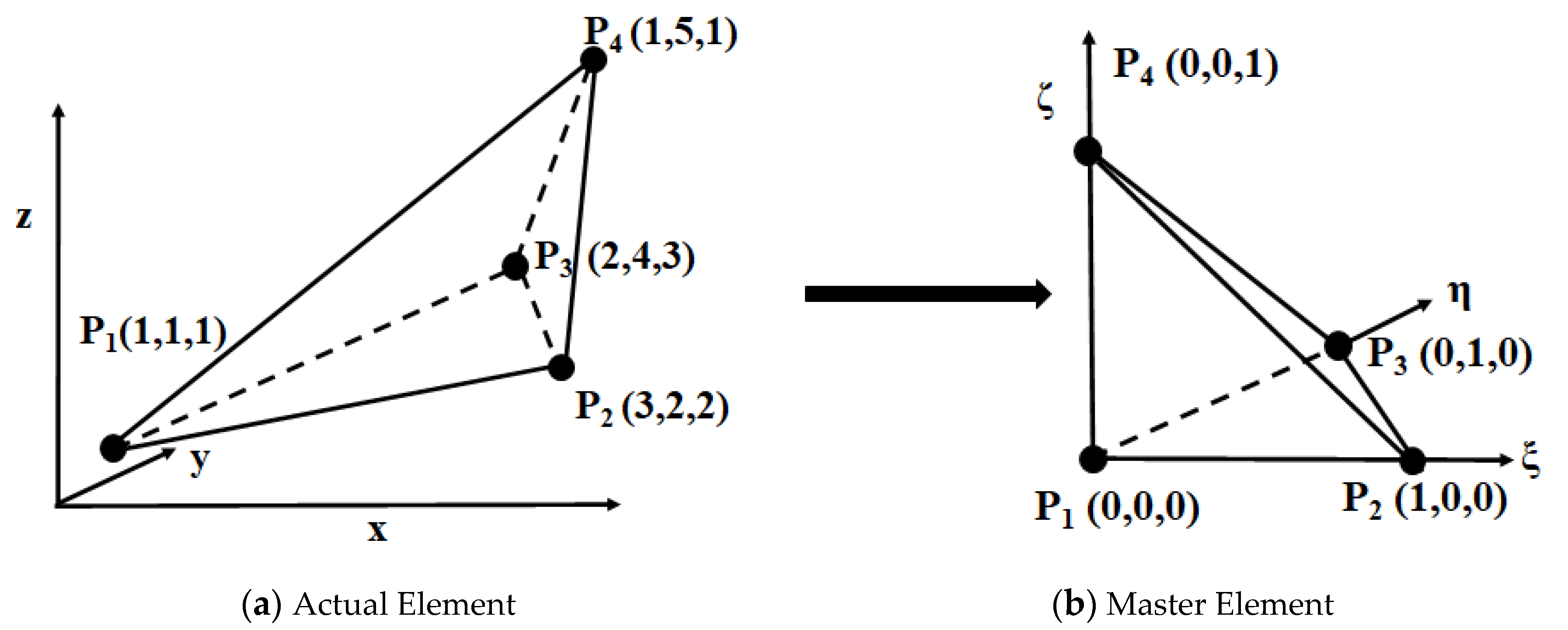
2.2. Transformation Formulation of Coordinates and Velocity Vectors between Actual and Mater Element

Arbitrary shape tetrahedron elements in Actual Element (x-y-z plane) are shown in Figure 1a, the geometrical is very complex for tracing a streamline, so it is very important to minimize the geometrical complexity. Therefore, tetrahedron elements in Actual Element need to transform into Master Element (ξ-η-ζ plane) where the geometrical complexity is minimized, as shown in Figure 1b, and the transform process schematic from Actual Element to Master Element is shown as Figure 1.

The first variable needed to transform between Master and Actual Elements is the coordinates. The coordinates in Actual Elements could transform to Master Elements easily by Equation (2), which only needs to take coordinates (x, y, z) into Equation (2) and replace U; the result is shown in Equation (5). The (x₁, y₁, z₁), (x₂, y₂, z₂), (x₃, y₃, z₃) and (x₄, y₄, z₄), are the coordinates of four vertexes of the tetrahedron in the Actual Element.

$$\begin{array}{l}x=\left(1-\xi -\eta -\zeta \right)x_1+\xi x_2+\eta x_3+\zeta x_4\\ y=\left(1-\xi -\eta -\zeta \right)y_1+\xi y_2+\eta y_3+\zeta y_4\\ z=\left(1-\xi -\eta -\zeta \right)z_1+\xi z_2+\eta z_3+\zeta z_4\end{array}$$

(5)

Then, transformation coordinates (x, y, z) in Actual Elements to coordinates (ξ, η, ζ) in Master Element is more complex. The transformation formulation is shown as Equation (6), which is derived from Equation (5).

$$\left[\begin{array}{l}\xi \\ \eta \\ \zeta \end{array}\right]={\left[\begin{array}{l}{x}_1-x_2{x}_1-x_3{x}_1-x_4\\ y_1-y_2{y}_1-y_3 y_1-y_4\\ z_1-z_2{z}_1-z_3{z}_1-z_4\end{array}\right]}^{-1}\left[\begin{array}{l}{x}_1-x\\ y_1-y\\ z_1-z\end{array}\right]$$

(6)

Another variable needed to transform between Actual and Master Elements is the velocity vector. For any given velocity vector [v_x, v_y, v_z] at a point (x, y, z) in an Actual Element, it needs to be transformed to the Master Element ([v_ξ, v_η, v_ζ]). According to Equation (6), the transformation formula for velocity vectors from an Actual Element to a Master Element is expressed as shown in Equation (7).

$$\left[\begin{array}{l}{\upsilon }_{\mathsf{\xi }}\\ {\upsilon }_{\mathsf{\eta }}\\ {\upsilon }_{\mathsf{\zeta }}\end{array}\right]=\left[\begin{array}{l}\frac{\partial \xi }{\partial x} \frac{\partial \xi }{\partial y} \frac{\partial \xi }{\partial z} \\ \frac{\partial \eta }{\partial x} \frac{\partial \eta }{\partial y} \frac{\partial \eta }{\partial z}\\ \frac{\partial \zeta }{\partial x} \frac{\partial \zeta }{\partial y} \frac{\partial \zeta }{\partial z}\end{array}\right]\left[\begin{array}{l}{\upsilon }_{\mathrm{x}}\\ {\upsilon }_{\mathrm{y}}\\ {\upsilon }_{\mathrm{z}}\end{array}\right]=-{\left[\begin{array}{l}{x}_1-x_2{x}_1-x_3{x}_1-x_4\\ y_1-y_2{y}_1-y_3 y_1-y_4\\ z_1-z_2{z}_1-z_3{z}_1-z_4\end{array}\right]}^{-1}\left[\begin{array}{l}{\upsilon }_{\mathrm{x}1}\\ {\upsilon }_{\mathrm{y}1}\\ {\upsilon }_{\mathrm{z}1}\end{array}\right]$$

(7)

2.3. The Analytical Solution for Describing the Trajectory in Master Element

In order to obtain the analytical solution for describing the trajectory in Master Element, it needs to know the motion equations at any point (ξ, η, ζ), that is to say, the velocity vector for any point is the key point. According to the shape function in the Master Element, the velocity vector of any point yields Equation (8), when the velocity vectors ([v_ξ1, v_η1, v_ζ1], [v_ξ2, v_η2, v_ζ2], [v_ξ3, v_η3, v_ζ3], and [v_ξ4, v_η4, v_ζ4]) at each vertex are obtained.

$$\begin{array}{l}{\upsilon }_{\mathsf{\xi }}=\frac{d\xi }{dt}={\upsilon }_{\mathsf{\xi }1}-\left({\upsilon }_{\mathsf{\xi }1}-{\upsilon }_{\mathsf{\xi }2}\right)\xi -\left({\upsilon }_{\mathsf{\xi }1}-{\upsilon }_{\mathsf{\xi }3}\right)\eta -\left({\upsilon }_{\mathsf{\xi }1}-{\upsilon }_{\mathsf{\xi }4}\right)\zeta \\ {\upsilon }_{\mathsf{\eta }}=\frac{d\eta }{dt}={\upsilon }_{\mathsf{\eta }1}-\left({\upsilon }_{\mathsf{\eta }1}-{\upsilon }_{\mathsf{\eta }2}\right)\xi -\left({\upsilon }_{\mathsf{\eta }1}-{\upsilon }_{\mathsf{\eta }3}\right)\eta -\left({\upsilon }_{\mathsf{\eta }1}-{\upsilon }_{\mathsf{\eta }4}\right)\zeta \\ {\upsilon }_{\mathsf{\zeta }}=\frac{d\zeta }{dt}={\upsilon }_{\mathsf{\zeta }1}-\left({\upsilon }_{\mathsf{\zeta }1}-{\upsilon }_{\mathsf{\zeta }2}\right)\xi -\left({\upsilon }_{\mathsf{\zeta }1}-{\upsilon }_{\mathsf{\zeta }3}\right)\eta -\left({\upsilon }_{\mathsf{\zeta }1}-{\upsilon }_{\mathsf{\zeta }4}\right)\zeta \end{array}$$

(8)

The initial conditions are shown in Equation (9).

$$\begin{array}{l}\xi \left(t=0\right)={\xi }_0;\eta \left(t=0\right)={\eta }_0;\zeta \left(t=0\right)={\zeta }_0\\ \frac{d\xi }{dt}(t=0)={\upsilon }_{\mathsf{\xi }0};\frac{d\eta }{dt}(t=0)={\upsilon }_{\mathsf{\eta }0};\frac{d\zeta }{dt}(t=0)={\upsilon }_{\mathsf{\zeta }0}\end{array}$$

(9)

Then, the matrix format of Equation (8) is described as shown in Equation (10):

$$\begin{array}{l}\frac{dX}{dt}=B+AX\\ X=\left(\begin{array}{l}\xi \\ \eta \\ \zeta \end{array}\right), B=\left(\begin{array}{l}{\upsilon }_{\mathsf{\xi }1}\\ {\upsilon }_{\mathsf{\eta }1}\\ {\upsilon }_{\mathsf{\zeta }1}\end{array}\right), A=\left(\begin{array}{l}-\left({\upsilon }_{\mathsf{\xi }1}-{\upsilon }_{\mathsf{\xi }2}\right) -\left({\upsilon }_{\mathsf{\xi }1}-{\upsilon }_{\mathsf{\xi }3}\right) -\left({\upsilon }_{\mathsf{\xi }1}-{\upsilon }_{\mathsf{\xi }4}\right)\\ -\left({\upsilon }_{\mathsf{\eta }1}-{\upsilon }_{\mathsf{\eta }2}\right) -\left({\upsilon }_{\mathsf{\eta }1}-{\upsilon }_{\mathsf{\eta }3}\right) -\left({\upsilon }_{\mathsf{\eta }1}-{\upsilon }_{\mathsf{\eta }4}\right)\\ -\left({\upsilon }_{\mathsf{\zeta }1}-{\upsilon }_{\mathsf{\zeta }2}\right) -\left({\upsilon }_{\mathsf{\zeta }1}-{\upsilon }_{\mathsf{\zeta }3}\right) -\left({\upsilon }_{\mathsf{\zeta }1}-{\upsilon }_{\mathsf{\zeta }4}\right)\end{array}\right)\end{array}$$

(10)

According to Gregory et al. [48], the general solution of Equation (11) is of the form

$$X(t)=E_1{\mathsf{\Phi }}_1\left(t\right)+E_2{\mathsf{\Phi }}_2\left(t\right)+E_3{\mathsf{\Phi }}_3\left(t\right)+C$$

(11)

where the particular function Φ₁(t), Φ₂(t) and Φ₃(t), and coefficients E₁, E₂, E₃, and C depend on the eigenvalues of A. There are nine separate cases that X(t) takes depending on different combinations eigenvalues. Here is Case 1 (Equation (12)), which means A has three nonzero real eigenvalues (0 ≠ r₁ ≠ r₂ ≠ r ₃≠ 0), and the other cases are shown in Appendix A.

(1) Case 1: A has three nonzero real eigenvalues (0 ≠ r₁ ≠ r₂ ≠ r₃ ≠ 0)

$$\begin{array}{l}X\left(t\right)=E_1{e}^{r_{1}t}+E_2{e}^{r_{2}t}+E_3{e}^{r_{3}t}+X_{\mathrm{c}}\\ E_1=\left(\frac{A-r_{2}I}{r_1-r_2}\right)\left(\frac{r_{3}I-A}{r_3-r_1}\right)\left(X_0-X_{\mathrm{c}}\right)\\ E_2=\left(\frac{A-r_{3}I}{r_2-r_3}\right)\left(\frac{r_{1}I-A}{r_1-r_2}\right)\left(X_0-X_{\mathrm{c}}\right)\\ E_3=\left(\frac{A-r_{1}I}{r_3-r_1}\right)\left(\frac{r_{2}I-A}{r_2-r_3}\right)\left(X_0-X_{\mathrm{c}}\right)\\ X_{\mathrm{c}}=-B{A}^{-1},X_0=\left(\begin{array}{l}{\xi }_0\\ {\eta }_0\\ {\zeta }_0\end{array}\right)\end{array}$$

(12)

2.4. Computing the TOF and Exit Coordinate

For any particle in the Mater Element whose start point is P₀, it will leave tetrahedron elements at exit points P_e on one face of the tetrahedron element. The time that the particle spends to leave the tetrahedron element from the start point to the exit point is TOF (Time of Flight), which is denoted by ∆τ. The ∆τ and P_e could be computed by the following steps.

Step 1: Calculation of the TOFs.

Assume that one fluid particle could leave a tetrahedron element from any face. Therefore, it is needed to compute the time that the particle spent from start point P₀ to each face, which is denoted by ∆τ₁, ∆τ₂, ∆τ₃, and ∆τ₄ to Face 1 (face P₂-P₁-P₄), Face 2 (face P₂-P₁-P₃), Face 3 (face P₃-P₁-P₄), and Face 4 (face P₂-P₃-P₄), respectively, which is shown in Figure 1b. Taking Case 1 (Section 2.3) as an example, for any given time, the coordinates can be computed; while for given coordinates, the time could be calculated by the Newton–Raphson method. So, when the position coordinate satisfies η = 0, the ∆τ₁ could be calculated, which yields Equation (13). In order to compute ∆τ₂, ∆τ₃, and ∆τ₄, the position coordinate should satisfy ζ = 0, ξ = 0 and ξ + η+ ζ = 1, yielding Equations (14)–(16), respectively.

$$0=\eta =E_{12}{e}^{r_1\Delta {\tau }_1}+E_{22}{e}^{r_2\Delta {\tau }_1}+E_{32}{e}^{r_3\Delta {\tau }_1}+P_{\mathrm{c}2}$$

(13)

$$0=\zeta =E_{13}{e}^{r_1\Delta {\tau }_2}+E_{23}{e}^{r_2\Delta {\tau }_2}+E_{33}{e}^{r_3\Delta {\tau }_2}+P_{\mathrm{c}3}$$

(14)

$$0=\xi =E_{11}{e}^{r_1\Delta {\tau }_3}+E_{21}{e}^{r_2\Delta {\tau }_3}+E_{31}{e}^{r_3\Delta {\tau }_3}+P_{\mathrm{c}1}$$

(15)

$$\begin{array}{ll}1=\xi +\eta +\zeta =& E_{11}{e}^{r_1\Delta {\tau }_4}+E_{21}{e}^{r_2\Delta {\tau }_4}+E_{31}{e}^{r_3\Delta {\tau }_4}+P_{\mathrm{c}1}\\ & +E_{12}{e}^{r_1\Delta {\tau }_4}+E_{22}{e}^{r_2\Delta {\tau }_4}+E_{32}{e}^{r_3\Delta {\tau }_4}+P_{\mathrm{c}2}\\ & +E_{13}{e}^{r_1\Delta {\tau }_4}+E_{23}{e}^{r_2\Delta {\tau }_4}+E_{33}{e}^{r_3\Delta {\tau }_4}+P_{\mathrm{c}3}\end{array}$$

(16)

Step 2: Determination of the real ∆τ from calculated TOFs.

Now, ∆τ₁, ∆τ₂, ∆τ₃, and ∆τ₄ have been calculated, but these TOFs may be negative or positive. According to the physical meaning of particle flow, the real ∆τ should be the minimum value of positive TOFs, which yields ∆τ = minPositive (∆τ₁, ∆τ₂, ∆τ₃ and ∆τ₄).

Step 3: Determination of the coordinate of P_e.

Now that the real TOF is determined, the exit coordinate (ξ_e, η_e, ζ_e) could be determined by the following equations.

$$\begin{array}{l}{\xi }_{\mathrm{e}}=E_{11}{e}^{r_1\Delta \tau }+E_{21}{e}^{r_2\Delta \tau }+E_{31}{e}^{r_3\Delta \tau }+P_{\mathrm{c}1}\\ {\eta }_{\mathrm{e}}=E_{12}{e}^{r_1\Delta \tau }+E_{22}{e}^{r_2\Delta \tau }+E_{32}{e}^{r_3\Delta \tau }+P_{\mathrm{c}2}\\ {\zeta }_{\mathrm{e}}=E_{13}{e}^{r_1\Delta \tau }+E_{23}{e}^{r_2\Delta \tau }+E_{33}{e}^{r_3\Delta \tau }+P_{\mathrm{c}3}\end{array}$$

(17)

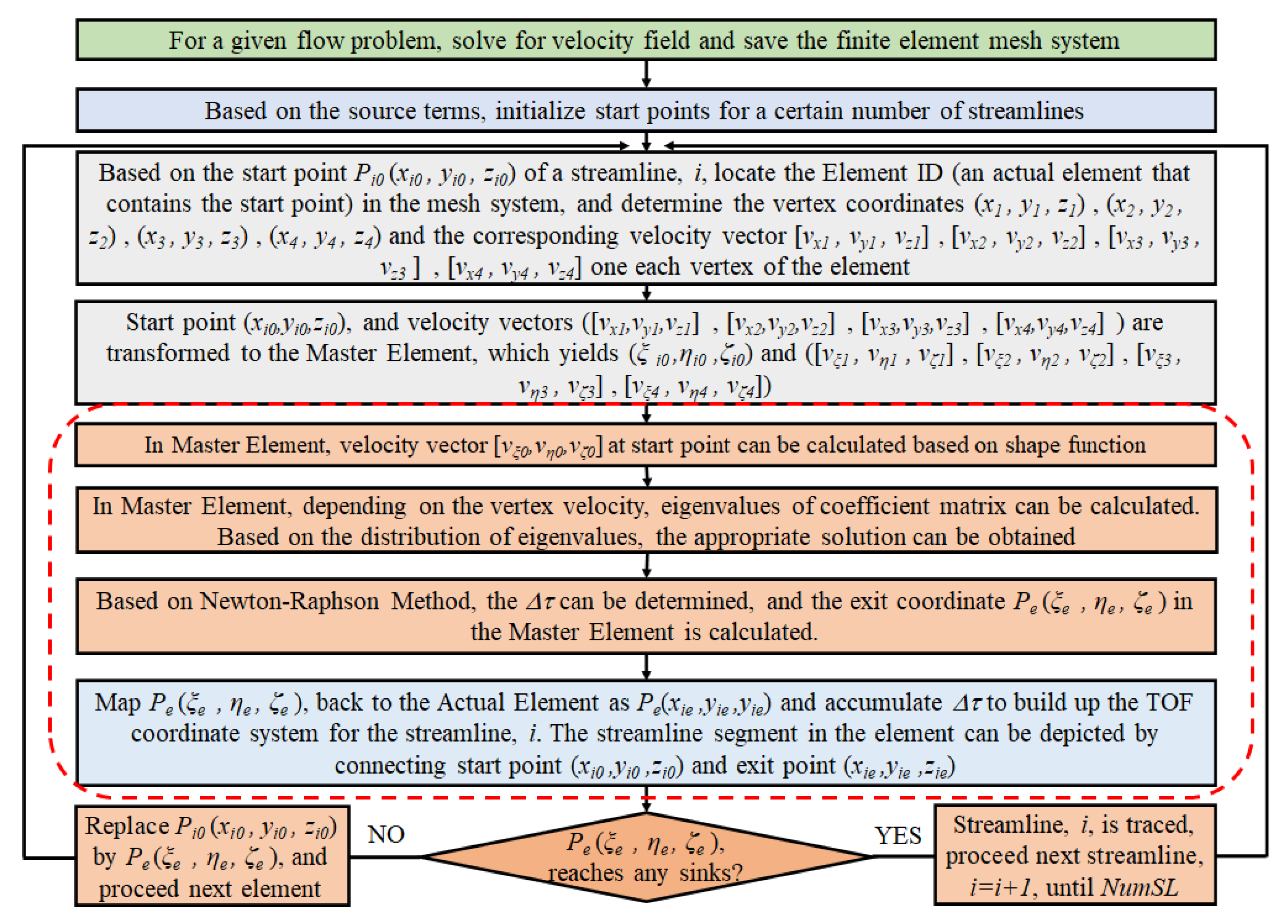
3. The Method to Trace Streamlines over Tetrahedron Grid Created by FEM

A new method is presented to trace streamlines over the tetrahedron grid system created by FEM, and the flowchart is shown in Figure 2. Based on a given velocity field, the process of tracing one streamline is shown in the steps below:

(1)

Import a tetrahedron mesh system created by FEM and the velocity field.

(2)

Give a start point P₀ in the x-y-z plane (Actual Element); then, find the cell where the start point is located, and obtain these element properties such as the coordinates on each vertex of the cell and the corresponding velocity vector.

(3)

Transform the coordinates and velocity vectors at four vertexes of the tetrahedron element.

(4)

Convert start point properties (such as velocity vector and coordinate) to the Master Element (ξ-η-ζ plane).

(5)

Trace a streamline in the tetrahedron element and determine the exit point P_e* coordinate and time (TOF) spent from start point to exit point in the Master Element.

(6)

Map the exit point coordinate P_e* (ξ_e, η_e, ζ_e) in Master Element back to Actual Element as P_e (x_e, y_e, z_e) and accumulate Δτ to construct the TOF coordinate system;

(7)

Check whether the exit point P_e reaches a sink or not. If yes, it means this streamline is traced successfully, and stop tracing this streamline. If does not reach, replace the start point P₀ by using the calculated exit point P_e and repeat Steps 2–7.

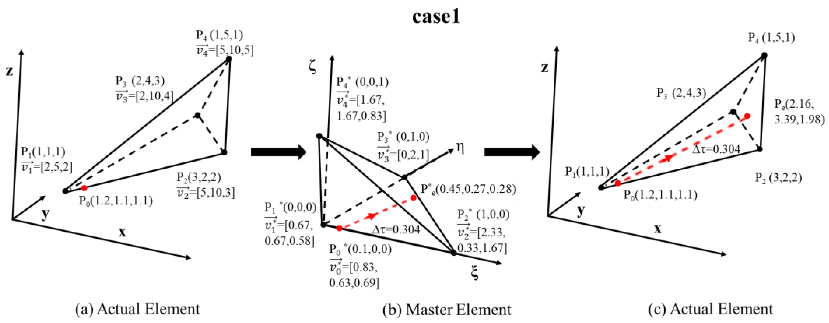
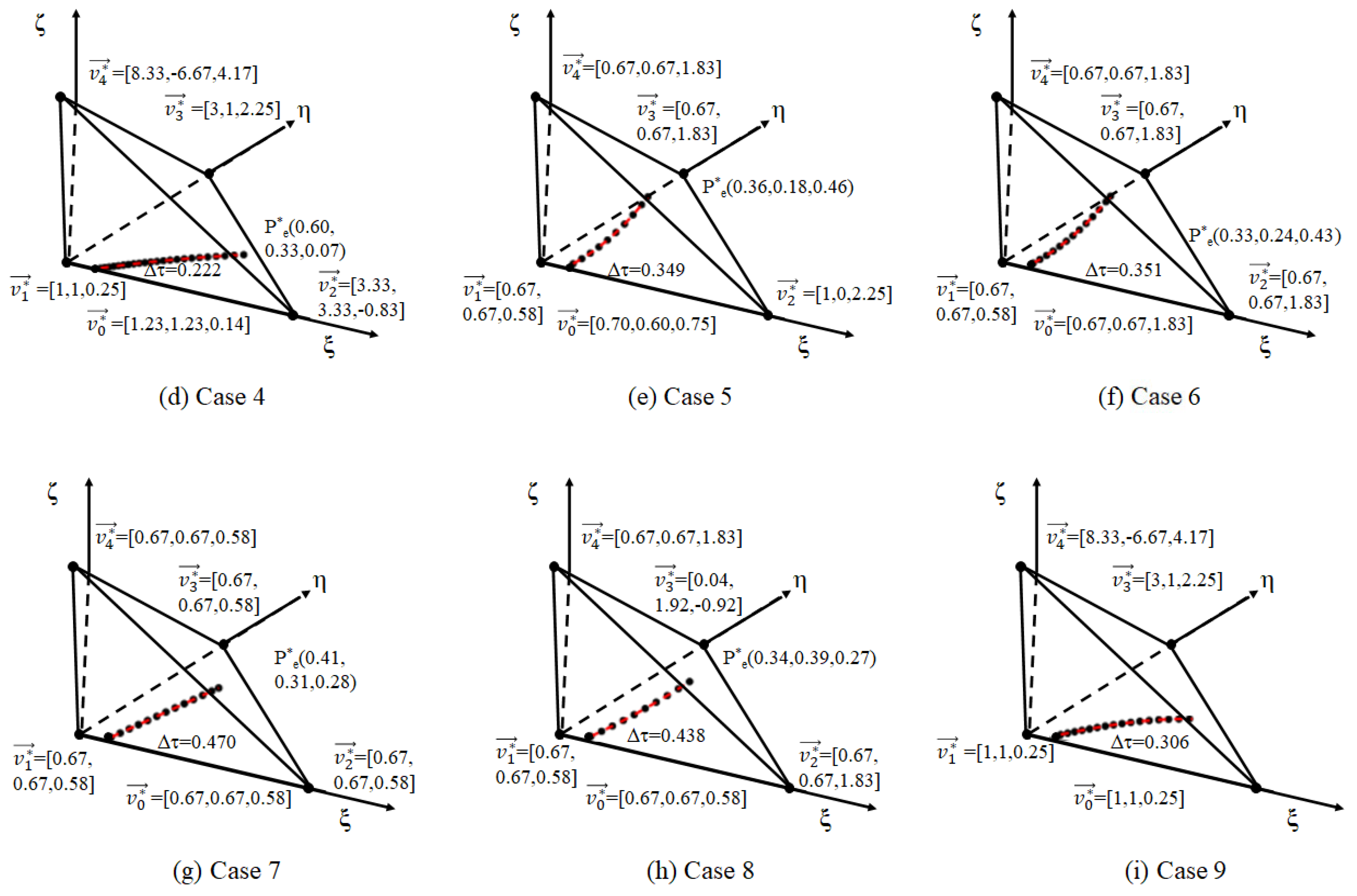
3.1. Tracing Streamline over a Tetrahedron Element

This subsection will elaborate how to trace a streamline over a tetrahedron element in an Actual Element, which includes Step 2 to Step 7.

In Step 2, for any given start point (P₀(x₀, y₀, z₀)) in the Actual Element, find the tetrahedron element where P₀ is located and obtain the parameters of this tetrahedron element, such as the coordinates of each vertex (P₁(x₁, y₁, z₁), P₂(x₂, y₂, z₂), P₃(x₃, y₃, z₃), P₄(x₄, y₄, z₄)) and velocity vectors on the each vertex ([v_x1, v_y1, v_z1], [v_x2, v_y2, v_z2], [v_x3, v_y3, v_z3], [v_x4, v_y4, v_z4]).

In Step 3, those parameters are used to calculate the start point (ξ₀, η₀, ζ₀) via Equation (5) and the velocity vector on each vertex ([v_ξ1, v_η1, v_ζ1], [v_ξ2, v_η2, v_ζ2], [v_ξ3, v_η3, v_ζ3], [v_ξ4, v_η4, v_ζ4] at ξ-η-ζ coordinate of (0,0,0), (1,0,0), (0,1,0), (0,0,1), respectively) in the Master Element via Equation (7).

In Step 4, based on the start point coordinate (ξ₀, η₀, ζ₀) and tetrahedron element properties (coordinates and velocity vectors at each vertex), the velocity vector [v_ξ0, v_η0, v_ζ0] at the start point can be calculated by the shape function. Now, the start points properties (coordinate and velocity vectors) and tetrahedron element properties (coordinate and velocity vectors at each vertex of the tetrahedron element) have been converted into Master Element.

In Step 5, now it is time to determine the pathway of a streamline over one tetrahedron element, noting that this is only a streamline segment. The equation for illuminating the trajectory of a streamline is presented in Section 2.3. When given a time, t, the position coordinate in the Master Element can be determined. Additionally, the TOF in one tetrahedron element could be calculated according the process expressed in Section 2.4. Then, the exit point coordinate could be calculated by taking the calculated TOF into the corresponding equation (such as Equation (17)).

In Step 6, Map the exit point coordinate P_e*(ξ_e, η_e, ζ_e) in Master Element back from to Actual Element as P_e(x_e, y_e, z_e) via Equation (6).

The procedure of tracing a streamline segment in a tetrahedron element and the relative formulations in Section 2.3 and Section 2.4 are demonstrated, which are verified by an example shown in Figure 3. A tetrahedron is defined in Actual Element with four vertices, which are P₁(1, 1, 1), P₂(3, 2, 2), P₃(1, 4, 3), and P₄(1, 5, 1) whose unit is m, respectively, as well as the corresponding velocity vector at four vertices are also given. When a particle starts from a start point which is located at one face of this tetrahedra element, then it will leave this tetrahedron element at an exit point. The procedure of tracing a streamline segment over a tetrahedron element in the Master Element is shown in Figure 3, which is referred to as Case 1, whose start point P₀(1.2, 1.1, 1.1) is located at Face 1 (Face P₁-P₂-P₄) of this tetrahedron element. The corresponding velocity vectors at four vertices of this tetrahedron element are v₁ = [2,5,2], v₂ = [5,10,3], v₃ = [2,10,4], and v₄ = [5,10,5], which yields Case 1, whose feature is that Equation (12) has three nonzero and real eigenvalues, as shown in Section 2.3. The velocities unit is m/s.

The geometrical sketch and parameters of a tetrahedron element in Actual Element (such as the coordinates and velocity vectors) are shown in Figure 3a. Then, coordinates and velocity vectors are transformed into Master Element via Equations (6) and (7), respectively, and the result is shown in Figure 3b. Thereby, the streamline pathway, Time of Flight (TOF) and the exit point coordinate P_e* are determined by relative formulations in Section 2.3 and Section 2.4; the result is also shown in Figure 3b. Finally, the results of the streamline segment (streamline pathway and exit point) could be converted to Actual Element, which is shown in Figure 3c. This example verified the procedure of tracing a streamline segment over a tetrahedron element.

The calculation results by relative formulations in Section 2.3 and Section 2.4 are verified by the RK4 method. The RK4 is the so-called fourth-order Runge–Kutta method, which is adopted to verify ODEs, since it is easily to implement during calculation. Equation (10) has nine cases according to the eigenvalue combination caused by the different velocity vectors at each vertex.

Figure 4 shows nine verification cases for Case 1 (three nonzero real eigenvalues shown as Equation (12), Case 2 (one real and two equal-nonzero real eigenvalues shown as Equation (A1)), Case 3 (a single nonzero real eigenvalue shown as Equation (A2)), Case 4 (one nonzero real and two complex eigenvalues shown as Equation (A3)), Case 5 (one zero real and two nonzero real eigenvalues shown as Equation (A4)), Case 6 (one nonzero real and two zero eigenvalues shown as Equation (A5)), Case 7 (only zero eigenvalues shown as Equation (A6)), Case 8 (one zero and two equal-nonzero real eigenvalues shown as Equation (A7)), Case 9 (two complex and one zero eigenvalues shown as Equation (A8)).

The comparison results are shown in Figure 4, including Case 2, where v₁ = [2,5,2], v₂ = [5.375,10,5], v₃ = [5,10,8], and v₄ = [2,10,2]; Case 3, where v₁ = [2,5,2], v₂ = [5,10,5], v₃ = [3,10,4] and v₄ = [2,9,2]; Case 4, where v₁ = [3,5,3], v₂ = [10,10,10], v₃ = [7,15,5] and v₄ = [10,5, −5]; Case 5, where v₁ = [2,5,2], v₂ = [2,10,1], v₃ = [2,10,2], and v₄ = [2,10,2]; Case 6, where v₁ = [2,5,2], v₂ = [2,10,2], v₃ = [2,10,2], and v₄ = [2,10,2]; Case 7, where v₁ = [2,5,2], v₂ = [2,5,2], v₃ = [2,5,2]; and v₄ = [2,5,2], Case 8, where v₁ = [2,5,2], v₂ = [2,5,2], v₃ = [2,5,3.875], and v₄ = [2,10,2], as well as Case 9 where v₁ = [3,5,3], v₂ = [3,5,3], v₃ = [7,15,5], and v₄ = [10,5,−5]. The velocities unit is m/s.

All the given velocities are in Actual Element, and all corresponding values are in Master Element, which is denoted as v₁*, v₂*, v₃*, and v₄* can be found in Figure 4. The streamline for different cases is calculated, and we compared the analytical solution and the 4th-order Runge–Kutta method, and the procedures of using the 4th-order Runge–Kutta method solve partial differential equation (such as Equation (10)), which is shown in Appendix B.

Despite RK4 having numerical errors, if reducing the value of Δt, the results will be convergent to an accurate solution. When Δt = 0.001 s, all the results of RK4 match perfectly with the result of the analytical solution, which is shown in Section 2.3 in this study. In addition, the TOFs (Δτ) calculated by RK4 give equal results in this study (value is shown in Figure 4). Although RK4 can also compute a streamlined pathway, the RK4 is not suited for streamline-based simulation due to its low efficiency and numerical errors.

As is shown in

Table 1. The calculation results and error of TOF by analytical solution and RK4 method for nine cases.

Case	TOF Calculated by Analytical Solution	TOF Calculated by RK4
		Δt = 0.01 s			Δt = 0.001 s			Δt = 0.0001 s
	TOF (s)	TOF (s)	Error (%)	Number of Iterations	TOF (s)	Error (%)	Number of Iterations	TOF (s)	Error (%)	Number of Iterations
Case 1	0.30432	0.3	1.42	450	0.304	0.105	4560	0.3043	0.007	45645
Case 2	0.30525	0.31	−1.556	465	0.305	0.082	4575	0.3051	0.049	45765
Case 3	0.32123	0.32	0.383	480	0.321	0.072	4815	0.3212	0.009	48180
Case 4	0.2214	0.22	0.632	330	0.221	0.181	3330	0.2213	0.045	33195
Case 5	0.34923	0.35	−0.22	375	0.349	0.066	5235	0.3491	0.037	52365
Case 6	0.35111	0.35	0.316	525	0.351	0.031	5265	0.3511	0.003	52665
Case 7	0.46956	0.47	−0.094	705	0.469	0.119	7035	0.4695	0.013	70425
Case 8	0.43823	0.44	−0.404	660	0.438	0.052	6570	0.4382	0.007	64920
Case 9	0.30615	0.31	−1.258	465	0.306	0.049	4590	0.3061	0.016	45915

, the error of TOF and the number of iterations by RK4 is up to large ∆t or small ∆t. Taking Case 1 as an example, when using small ∆t(∆t = 0.0001s), the RK4 could calculate an accurate TOF (error of TOF is 0.007%), but it needs to repeat 45645 iterations; while using large ∆t(∆t = 0.01s), the number of iterations decreased drastically (only 450 iterations), but the error of TOF is 1.42%, which is bigger. Considering the efficiency and the accuracy, 0.001 s is selected to calculate TOF by RK4, which was used to verify the analytical solution. Table 1 implies that although RK4 could determine the trajectory and TOF, there are some problems limiting its applications. (1) The computational accuracy and efficiency depend on the step(∆t) size. A small ∆t could determine an accurate TOF and coordinate, which decrease the computational efficiency, while a large ∆t could increase the computational efficiency but could not determine an accurate TOF and coordinate. (2) When tracing streamlines in the entire domain, only TOF and exit coordinates are needed to calculate each element, and it is not significant to know the detailed trajectory in one element. However, it requires repeating a large number of iterations to determine the TOF and exit coordinate by the RK4 method compared to only a few iterations in the analytical solution method; the process of determining the exit points and TOF by the analytical solution method is outlined in Section 2.4.

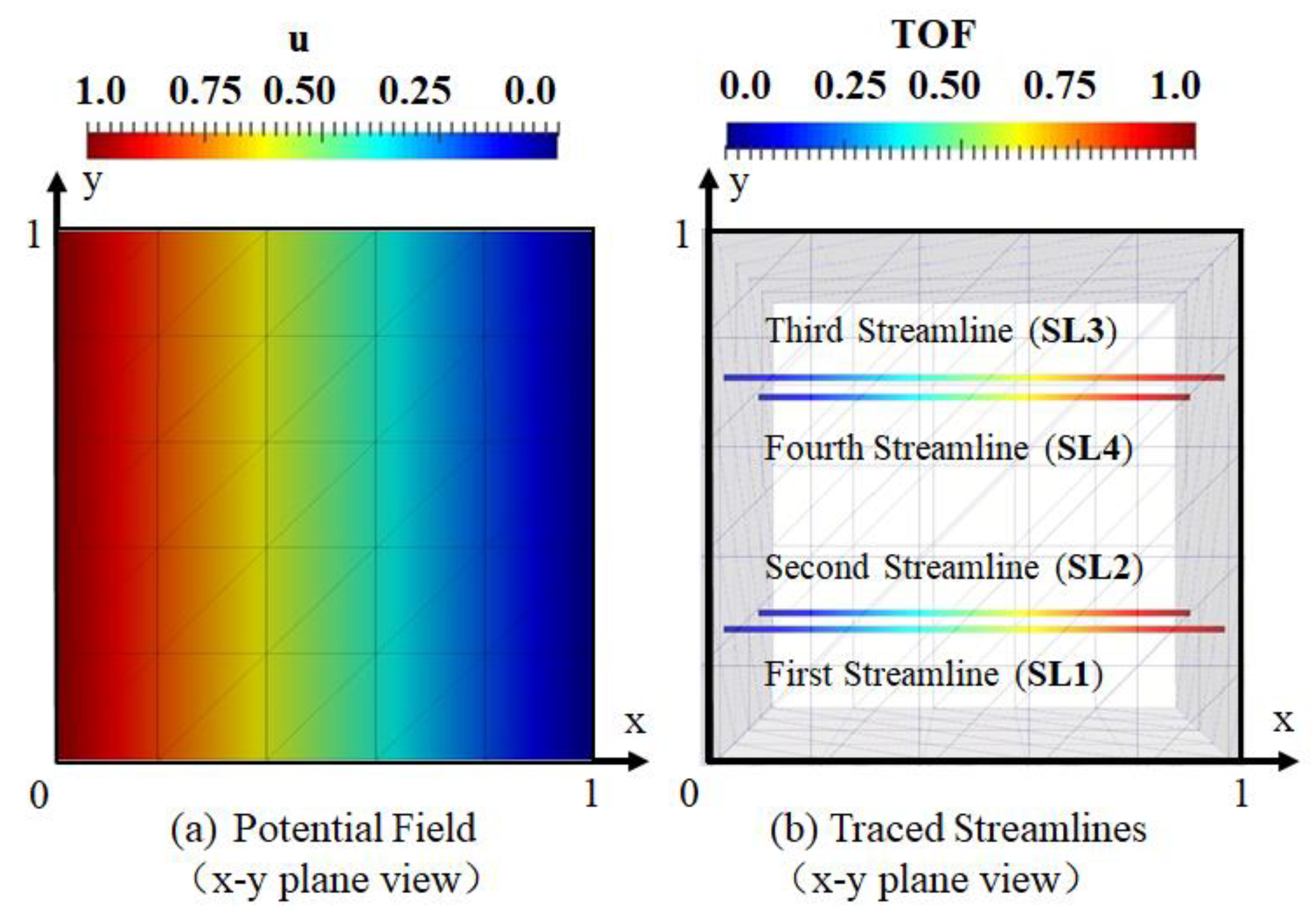
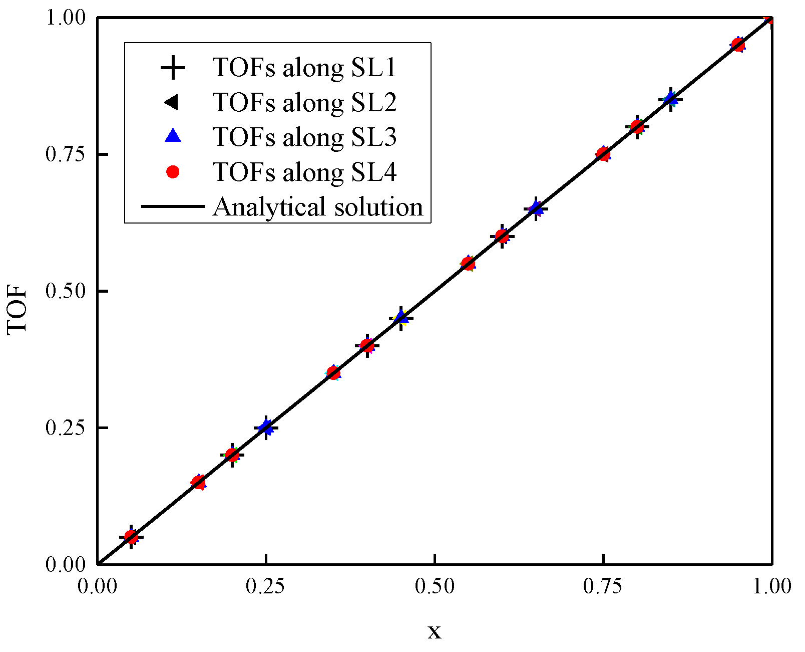
3.2. Tracing Streamline over the Whole Domain

This subsection demonstrates the process of tracing streamlines in the whole domain and building up a streamline system. After tracing a streamline over a tetrahedron element, it is important to make sure whether the exit point reaches the sink or not. If yes, this streamline is the end. However, if it does not, take the exit point as the start point in the next element and repeat the step of tracing a streamline over a tetrahedron element until the exit point reaches the sink. One streamline is formed by connecting the start point and exit point in each tetrahedron element. The process of tracing streamlines for the whole domain is verified by Case 1, which is shown in Section 4.1.

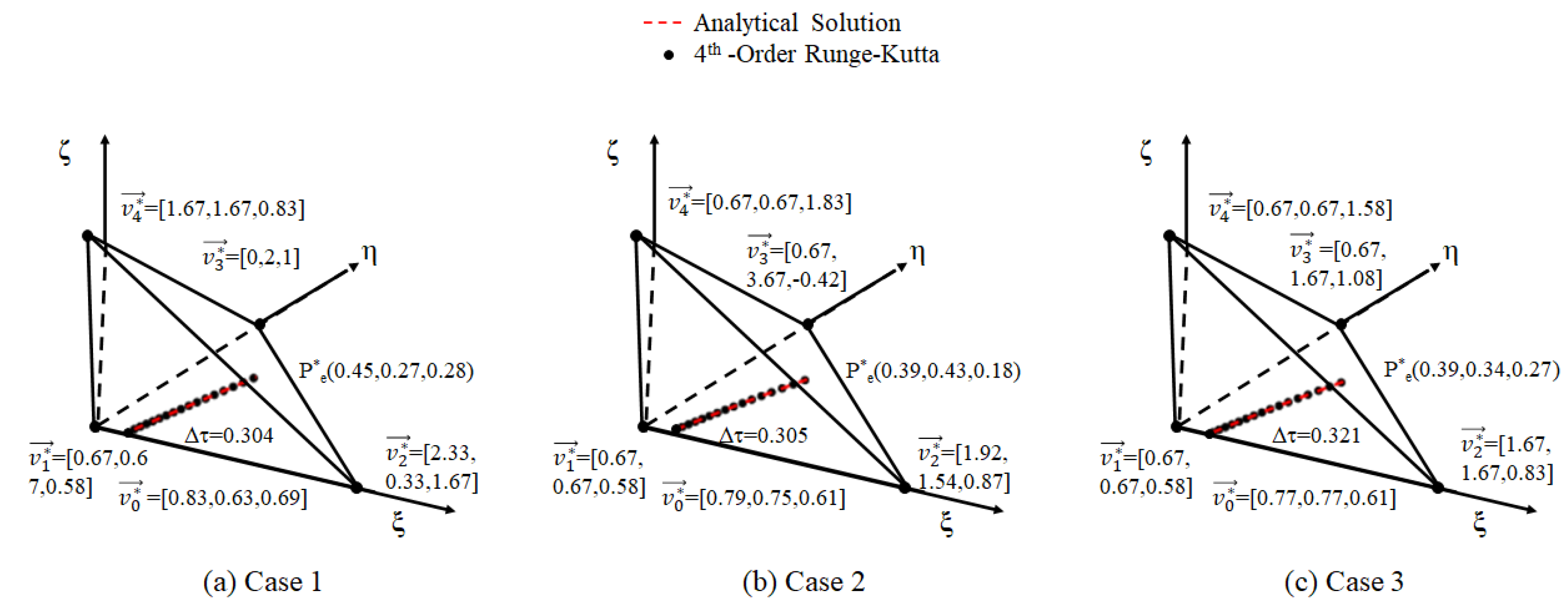
4. Results and Discussion

Some cases are studied to verify the process of tracing streamlines for the whole domain and illustrate the computational power of the method presented in this paper about tracing streamlines. The purpose of this paper is to propose a general tracing streamline method, so it does not involve any specific physical problems. The following case is based on the Laplace type equation, and the velocity and TOFs are calculated, but not in units. The flow field of the case in this paper is achieved in FEniCS; the details about FEniCS are shown in https://fenicsproject.org. The streamline tracing method in this paper is implemented via the FEniCS framework.

4.1. Case 1

The process of tracing streamlines for the whole domain is verified by a simple fluid flow problem (reference as Case 1), which is shown in Figure 5. Figure 5a is showing a simple fluid flow field of u in a unit cubic domain whose governing equation is Laplace’s equation, ∇²u = 0, where u, which is scalar, represents the potential field, and υ represents the velocity vector υ = −∇u. The boundary conditions are the Neumann boundary condition and Dirichlet boundary condition, where the Dirichlet boundary condition is applied to the left face (u = 1 when x = 0, y and z equal any values) and the right face (u = 0 when x = 1, y and z equal any values), while the Neumann boundary condition is applied to the top face (∂u/∂n = 0 when y = 1, x and z equal any values), bottom face ((∂u/∂n = 0 when y = 0, x and z equal any values), front face (∂u/∂n = 0 when z = 0, x and y equal any values) and the back face (∂u/∂n = 0 when z = 0, x and y equal any values). So, the flow field (u) in a unit cubic domain is distributed linearly from 1 to 0, which leads to a uniform velocity vector [v_x = 1, v_y = 0, v_z = 0]. Therefore, the streamlines of this flow field are a set of parallel straight lines, such as SL1, SL2, SL3, and SL4 shown in Figure 5b, whose start points are at (0.0, 0.25, 0.25), (0.0, 0.25, 0.75), (0.0, 0.75, 0.25) and (0.0, 0.75, 0.75), respectively.

As the velocity field is a uniform velocity vector, the TOF of one streamline is linear distributed from 0 at the left face boundary (x = 0) to 1 at the right face (x = 1), which means the analytical solution of TOF of one streamline could be represented as a line (slope equals one) on the graph of the relationship between TOF and x. Therefore, the TOF of this study could be verified by an exact solution, which is shown in Figure 5b as the solid line. As is shown in Figure 6, the TOFs of four streamlines are in perfect agreement with the analytical solution of TOFs on the plot of TOF and x, which means the new streamline tracing method over the tetrahedron mesh system presented in this paper is accurate.

4.2. Case 2

Case 2 is used to study the computational power of tracing a streamline in a vertical direction and horizontal direction, respectively. The purpose of this paper is to propose a general tracing streamline method, so it does not involve any specific physical problems.

Case 2 is shown in Figure 7, the calculation domain is a cube with length equaling 1.0, the governing equation is a Laplace equation, whose boundary condition is that the six faces of cube under the no-flow Neumann boundary condition (∂u/∂n = 0), and the source and sink are under the Dirichlet boundary condition (u = 1 and u = 0, respectively). The source is noted as a cylinder whose top coordinate is (0.1, 0.1, 1.0), bottom coordinate is (0.1, 0.1, 1.0), and radius is 0.05, while the sink is noted as a cylinder whose top coordinate is (0.9, 0.9, 1.0), bottom coordinate is (0.9, 0.9, 0.0), and radius is 0.05.

The discretization of the calculation domain is shown in Figure 7a. In the FEniCS framework, the resolution of a mesh system is determined via specifying a resolution number instead of the average mesh size, such as the ’20′ in code “mesh = generate_mesh(geometry, 20)”. The calculation domain was discretized into 8595 elements. Then, the Laplace equation is solved by FEniCS with boundary conditions in the calculation domain, and it extends the program to compute potential field (u), which is shown in Figure 7a.

Figure 7b presents the result of tracing 100 streamlines whose start points are located at the surface of the source and linearly distributed along the direction of the cylinder centerline. The TOF color map in Figure 7b,c shows the traveling time of a particle spending from the start point to the sink. Near the start point, the color of the streamline is blue, while near the sink, the color of the streamline is red. In Figure 7b, all the streamlines could start from the start point and reach the surface of the sink, which implies that the new method can trace the streamline in the vertical direction successfully.

Figure 7c shows that 100 streamlines were traced in the horizontal direction. The start points of 100 streamlines in Figure 7c are evenly distributed along the horizontal direction at the surface of the source, and all the z coordinates of start points equal 0.5. As shown in Figure 7c, 100 streamlines along the horizontal direction are traced successfully and are evenly distributed on a plane (whose plane equation is z = 0.5), which means that the method for tracing a streamline over the tetrahedron grid system presented in this study can trace all the streamlines in the horizontal direction.

According to the streamline tracing results in Figure 7b,c, the method to tracing a streamline over the tetrahedron grid system presented in this study is a robust method.

4.3. Case 3

The method for tracing a streamline over the tetrahedron grid system presented in this study could trace all the streamlines in both the vertical direction and horizontal direction, as implied from Case 2. However, the computational power of the algorithm is not studied when there is an obstacle in the computation domain. So, Case 3 is introduced, where an impermeable sphere is artificially introduced to add computational complexity. The center of the sphere is at (0.5, 0.5, 0.5), and the sphere radius is 0.4. The boundary condition at the surface sphere is the Neumann boundary condition ((∂u/∂n = 0), the boundary conditions are same as those in Case 2. Figure 8a shows the discretization of the calculation domain and the potential field (u), which represents that the fluids flow from the source and bypass the obstacles before finally flowing out from the sink. Figure 8b shows 100 streamlines (10 layers in the vertical direction, 10 streamlines launched in the horizontal direction) are traced successfully, and all the streamlines start from the source, then steer by obstacles and reach the sink.

5. Conclusions

In this paper, a new method to trace streamlines over unstructured tetrahedron elements based on vertex velocities is presented. The following conclusion are drawn:

(1)

The exit coordinate leaving a tetrahedral element and the Time of Flight (TOF) could be computed accurately and efficiently because the analytical solution that could depict the trajectory in Master Element is deduced.

(2)

Two verification cases are studied, whose results are agreeing to the new method to trace streamlines over unstructured tetrahedron elements based on vertex velocities. One of the verifications verifies the analytical solution for depicting the trajectory in Master Element by comparing it with the results of the RK4 method, while the other one verifies the process of tracing streamlines in the entire domain.

(3)

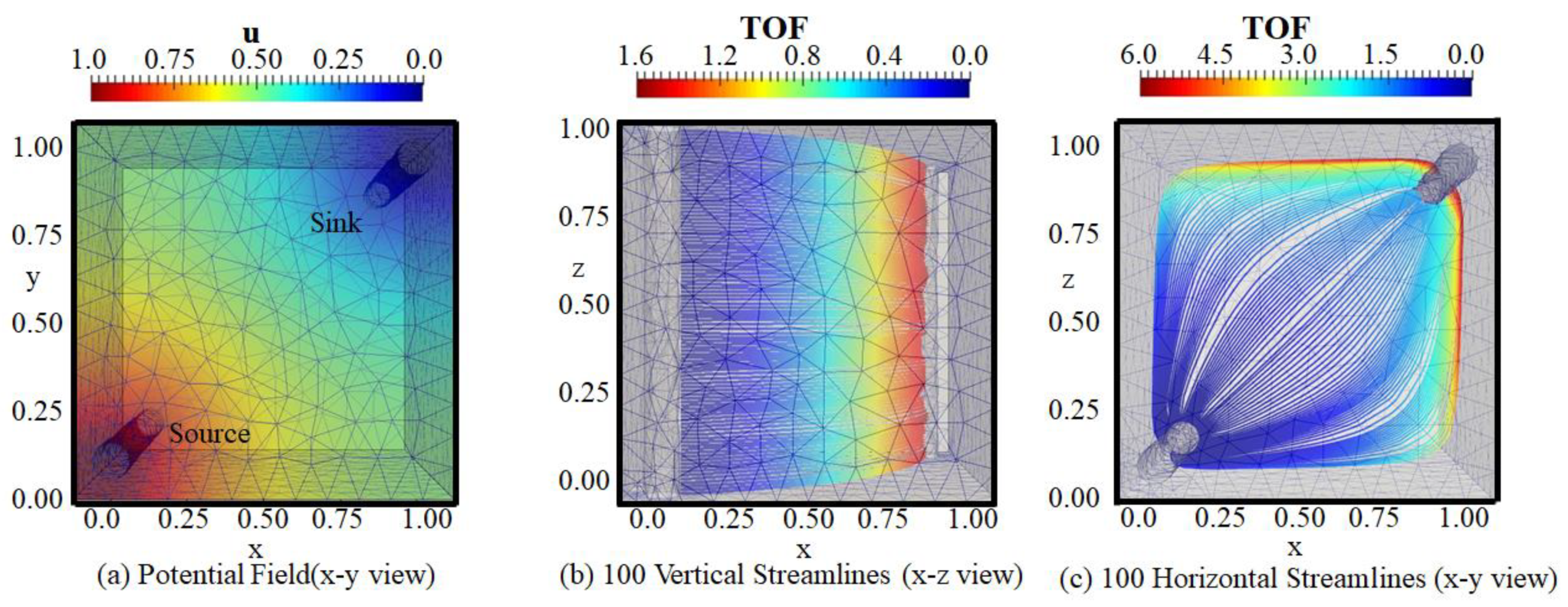
Two cases with different geometric complexity are studied to demonstrate the computational power of the method presented in this paper. The new method to trace streamlines over unstructured tetrahedron elements is a robust method that can handle a complex computational domain.

(4)

The presented method is implemented in FEniCS, which is a programming framework for Finite Element Method (FEM) that can be easily extend the method to other research fields. If the velocity field and tetrahedron mesh system are obtained during any fluid field solving in FEniCS, the new method can trace the streamlines of this fluid field, which can easily extend the method to other research fields.

References

1. Gautier, Y.; Noetinger, B.; Roggero, F. History Matching Using a Streamline-Based Approach and Gradual Deformation. SPE J. 2004, 9, 88–101. [Google Scholar] [CrossRef]
2. Singh, A.P.; Knabe, S.P.; Maucec, M. History Matching Using Streamline Trajectories. In Proceedings of the Abu Dhabi International Petroleum Exhibition & Conference, Abu Dhabi, UAE, 10–13 November 2013; Society of Petroleum Engineers (SPE): London, UK, 2014; pp. 10–13. [Google Scholar]
3. Ramirez, W.F. Application of Optimal Control Theory to Enhanced Recovery; Development of Petroleum Science series; Elsevier Science: New York, NY, USA, 1987; Volume 21. [Google Scholar]
4. Siavashi, M.; Tehrani, M.R.; Nakhaee, A. Efficient Particle Swarm Optimization of Well Placement to Enhance Oil Recovery Using a Novel Streamline-Based Objective Function. J. Energy Resour. Technol. 2016, 138, 052903. [Google Scholar] [CrossRef]
5. Zhu, Z.; Gerritsen, M.; Thiele, M. Thermal Streamline Simulation for Hot Waterflooding. SPE Reserv. Eval. Eng. 2010, 13, 372–382. [Google Scholar] [CrossRef]
6. Wen, T.; Thiele, M.R.; Ciaurri, D.E.; Aziz, K.; Ye, Y. Waterflood management using two-stage optimization with streamline simulation. Comput. Geosci. 2014, 18, 483–504. [Google Scholar] [CrossRef]
7. Batycky, R.P. A Three-Dimensional Two-Phase Field Scale Streamline Simulator. Ph.D. Thesis, Stanford University, Stanford, CA, USA, 1997. [Google Scholar]
8. Alsofi, A.M.; Blunt, M.J. Streamline-Based Simulation of non-Newtonian Poly Flooding. SPE J. 2010, 15, 895–905. [Google Scholar] [CrossRef]
9. Huang, W.; di Donato, G.; Blunt, M.J. Comparison of streamline-based and grid-based dual porosity simulation. J. Pet. Sci. Eng. 2004, 43, 129–137. [Google Scholar] [CrossRef]
10. Park, C.; Kang, J.M.; Jung, Y.; Kim, S. Streamline-based simulation to investigate interwell connectivity and tracer transport in 3D discrete fractured reservoir. In Proceedings of the SPE Europec/EAGE Annual Conference and Exhibition, Vienna, Austria, 12–15 June 2006. [Google Scholar]
11. Atchley, A.L.; Maxwell, R.M.; Navarre-Sitchler, A.K. Using streamlines to simulate stochastic reactive transport in heterogeneous aquifers: Kinetic metal release and transport in CO2 impacted drinking water aquifers. Adv. Water Resour. 2013, 52, 93–106. [Google Scholar] [CrossRef]
12. Qi, R.; la Force, T.; Blunt, M.J. A three-phase four-component streamline-based simulator to study carbon dioxide storage. Comput. Geosci. 2009, 13, 493–509. [Google Scholar] [CrossRef]
13. Crane, M.J.; Blunt, M.J. Streamline-based simulation of solute transport. Water Resour. Res. 1999, 35, 3061–3078. [Google Scholar] [CrossRef]
14. Maxwell, R.M.; Welty, C.; Tompson, A.F.B. Streamline-based simulation of virus transport resulting from long term artificial recharge in a heterogeneous aquifer. Adv. Water Resour. 2003, 26, 1075–1096. [Google Scholar] [CrossRef]
15. Di Donato, G.; Blunt, M.J. Streamline-based dual-porosity simulation of reactive transport and flow in fractured reservoirs. Water Resour. Res. 2004, 40, 1–12. [Google Scholar] [CrossRef]
16. Obi, E.-O.; Blunt, M.J. Streamline-based simulation of advective–dispersive solute transport. Adv. Water Resour. 2004, 27, 913–924. [Google Scholar] [CrossRef]
17. Herrera, P.A.; Valocchi, A.J.; Beckie, R.D. A multidimensional streamline-based method to simulate reactive solute transport in heterogeneous porous media. Adv. Water Resour. 2010, 33, 711–727. [Google Scholar] [CrossRef]
18. Batycky, R.P.; Thiele, M.R. Technology Update: Mature Flood Surveillance Using Streamlines. J. Pet. Technol. 2016, 68, 22–25. [Google Scholar] [CrossRef]
19. Zefreh, M.G.; Nilsen, H.M.; Lie, K.; Raynaud, X.; Doster, F. Streamline simulation of a reactive advective flow with discontinuous flux function. Comput. Geosci. 2018, 23, 255–271. [Google Scholar] [CrossRef] [Green Version]
20. Caudle, B.H. Fundamentals of Reservoir Engineering; Society of Petroleum: Richardson, TX, USA, 1967. [Google Scholar]
21. Collins, R.E. Japanese research in flow of fluids through porous materials and filtration. Trans. Am. Geophys. Union 1964, 45, 151–164. [Google Scholar] [CrossRef]
22. Lin, J.K. An Image well Method for Bounding Arbitrary Reservoir Shapes in the Streamline Model. Ph.D. Thesis, University of Texas at Austin, Austin, TX, USA, 1972. [Google Scholar]
23. Thiele, M.R. Modeling Multiphase Flow in Heterogeneous Media Using Streamtubes. Ph.D. Thesis, Stanford University, Stanford, CA, USA, 1994. [Google Scholar]
24. Datta-Gupta, A.; King, M.J. A semi analytical approach to tracer flow modeling in heterogeneous permeable media. Adv. Water Res. 1995, 18, 9–29. [Google Scholar] [CrossRef]
25. Thiele, M.R. Streamline simulation. In 6th International Forum on Reservoir Simulation; Schloss Fuschl: Salzburg, Austria, 2001. [Google Scholar]
26. Datta-Gupta, A.; King, M.J. Streamline Simulation: Theory and Practice; Society of Petroleum Engineering: Houston, TX, USA, 2007. [Google Scholar]
27. Hægland, H.; Dahle, H.; Eigestad, G.; Lie, K.-A.; Aavatsmark, I. Improved streamlines and time-of-flight for streamline simulation on irregular grids. Adv. Water Resour. 2007, 30, 1027–1045. [Google Scholar] [CrossRef]
28. Numbere, D.T. A General Streamline Modeling Technique for Homogeneous Porous with Application to Streamflood Prediction. Ph.D. Thesis, University of Oklahoma, Norman, OK, USA, 1982. [Google Scholar]
29. Pollock, D.W. Semianalytical Computation of Path Lines for Finite-Difference Models. Ground Water 1988, 26, 743–750. [Google Scholar] [CrossRef]
30. Prévost, M.; Edwards, M.G.; Blunt, M.J. Streamline Tracing on Curvilinear Structured and Unstructured Grids. SPE J. 2002, 7, 139–148. [Google Scholar] [CrossRef]
31. Juanes, R.; Matringe, S.F. Unified formulation for highorder streamline tracing on two-dimensinal unstructured grids. J. Sci. Comput. 2008, 38, 50–73. [Google Scholar] [CrossRef]
32. Zhang, Y.; King, M.J.; Datta-Gupta, A. Robust streamline tracing using inter-cell fluxes in locally refined and unstructured grids. Water Resour. Res. 2012, 48, 1–19. [Google Scholar] [CrossRef] [Green Version]
33. Siavashi, M.; Blunt, M.J.; Raisee, M.; Pourafshary, P. Three-dimensional streamline-based simulation of non-isothermal two-phase flow in heterogeneous porous media. Comput. Fluids 2014, 103, 116–131. [Google Scholar] [CrossRef]
34. Zuo, L.; Lim, J.; Chen, R.; King, M. Efficient Calculation of Flux Conservative Streamline Trajectories on Complex and Unstructured Grids. In Proceedings of the 78th EAGE Conference and Exhibition 2016, Vienna, Austria, 30 May–2 June 2016; EAGE Publications: Vienna, Austria. [Google Scholar]
35. Vasco, D.W.; Pride, S.R.; Zahasky, C.; Benson, S.M. Calculating Trajectories Associated with Solute Transport in a Heterogeneous Medium. Water Resour. Res. 2018, 54, 6890–6908. [Google Scholar] [CrossRef] [Green Version]
36. Wang, B.; Feng, Y.; Du, J.; Wang, Y.; Wang, S.; Yang, R. An Embedded Grid-Free Approach for Near-Wellbore Streamline Simulation. SPE J. 2018, 23, 567–588. [Google Scholar] [CrossRef]
37. Cordes, C.; Kinzelbach, W. Continuous groundwater velocity fields and path lines in linear, bilinear, and trilinear finite element. Water Resour. Res. 1992, 28, 2903–2911. [Google Scholar] [CrossRef]
38. Ham, D.A.; Pietrzak, J.; Stelling, G.S. A streamline tracking algorithm for semi-Lagrangian advection schemes based on the analytic integration of the velocity field. J. Comput. Appl. Math. 2006, 192, 168–174. [Google Scholar] [CrossRef] [Green Version]
39. Matringe, S.F.; Juanes, R.; Tchelepi, H.A. Streamline Tracing on General Triangular or Quadrilateral Grids. SPE J. 2007, 12, 217–233. [Google Scholar] [CrossRef]
40. Park, C.; Kang, J.M. Characterization of Tracer Transport in Heterogeneous Fractured Reservoir by a Streamline Approach on Unstructured Grids. Energy Sources 2008, 30, 856–871. [Google Scholar] [CrossRef]
41. Klausen, R.A.; Rasmussen, A.F.; Stephansen, A.F. Velocity interpolation and streamline tracing on irregular geometries. Comput. Geosci. 2011, 16, 261–276. [Google Scholar] [CrossRef]
42. Painter, S.L.; Gable, C.W.; Kelkar, S. Pathline tracing on fully unstructured control-volume grids. Comput. Geosci. 2012, 16, 1125–1134. [Google Scholar] [CrossRef]
43. Hao, J.; Wang, W.; Duo, Z. An efficient algorithm for streamline visualization in unstructured steady vector field. In Proceedings of the 2nd International Conference on Computer Science and Application Engineering, Hohhot, China, 22–24 October 2018. [Google Scholar]
44. Yin, F.; Erxiu, S.; Yi, L.; Bin, W.; Liehui, Z.; Yulong, Z. Implementation of streamline simulation based on finite element method in FEniCS. Comput. Geosci. 2019, 24, 1–5. [Google Scholar]
45. Bonduà, S.; Bortolotti, V. A tool for pathline creation using TOUGH simulation results and fully unstructured 3D Voronoi grids. Environ. Model. Softw. 2019, 115, 63–75. [Google Scholar] [CrossRef]
46. Craig, J.; Ramadhan, M.; Muffels, C. A Particle Tracking Algorithm for Arbitrary Unstructured Grids. Ground Water 2019, 58, 19–26. [Google Scholar] [CrossRef] [PubMed]
47. Batista, D. Mesh-independent streamline tracing. J. Comput. Phys. 2020, 401, 108967. [Google Scholar] [CrossRef]
48. Gregory, M.N.; II-Hong, J. Tools for computing tangent curves for linearly baring vector fields over tetrahedral domains. IEEE Trans. Vis. Comput. Graph. 1999, 5, 360–372. [Google Scholar]
Figure 1. The transform process schematic for coordinate of the Actual Element and Master Element where (a) represents tetrahedron in the Actual Element and (b) represents the tetrahedron in the Master Element.
Energies 13 06027 g001
Figure 2. The flowchart of tracing a streamline over the tetrahedron grid system created by Finite Element Method (FEM).
Energies 13 06027 g002
Figure 3. The procedure of tracing a streamline in a tetrahedron element generated by FEM. (a) The coordinates and velocity vectors at each vertex and the start point over a tetrahedron element in Actual Element. (b) The results of coordinates and velocity vectors transformed to Master Element and a streamline trajectory from the start point to the exit point in the Master Element, as well as the Time of Flight (TOF). (c) The streamline trajectory and coordinates of each vertex, start point, and exit point, which mapped back to Actual Element.
Energies 13 06027 g003
Figure 4. The comparison of this study result (solid lines) and RK4 result (discrete points) for different cases in Master Element. (ai) represents the result of comparison trajectory between this study and RK4 for Case 1, Case 2, Case 3, Case 4, Case 5, Case 6, Case 7, Case 8, and Case 9, respectively.
Energies 13 06027 g004aEnergies 13 06027 g004b
Figure 5. The simple fluid flow problem (Case 1) to verify the process of tracing streamlines for the whole domain where (a) shows the fluid field, u, and (b) shows four traced streamlines whose start points are at (0.0,0.25,0.25), (0.0,0.25,0.75), (0.0,0.75,0.25), and (0.0,0.75,0.75), respectively.
Energies 13 06027 g005
Figure 6. Comparison between analytical TOF shown as solid line and the calculated TOFs along four streamlines (SL1, SL2, SL3, and SL4) shown as discrete points.
Energies 13 06027 g006
Figure 7. The result of Case 2. (a) The discretization of the calculation domain and the potential field (u), (b,c) show the streamline pattern from the x-y plane view and x-z plane view, respectively.
Energies 13 06027 g007
Figure 8. The result of Case 3. (a) The discretization of the calculation domain and the potential field (u), and (b) streamline pattern from the x-y plane view.
Energies 13 06027 g008