Abstract
It is commonly believed that matrix and natural fractures randomly distribute in carbonate gas reservoirs. In order to increase the effective connected area to the storage space as much as possible, highly deviated wells are widely used for development. Although there have been some studies on the composite model for highly deviated wells, they have not considered the effects of stress sensitivity and threshold pressure gradient in a dual-porosity gas reservoir. In this paper, a semi-analytical composite model for low permeability carbonate gas reservoir was established to study the effect of non-Darcy flow. By employing source function, Fourier transform and the perturbation method, the pressure performance and typical well test curves were obtained. Eight flow regimes were identified, and their characteristics were discussed. As a result, it can be concluded that the effects of stress sensitivity and threshold pressure gradient would make pseudo-pressure and derivative curves rise, which is the characteristic of non-Darcy flow to determine whether there is stress sensitivity or threshold pressure gradient.
1. Introduction
Increasing global energy demand and recent advances in drilling techniques for highly deviated wells have accelerated the exploration and development of the carbonate gas reservoir. It has been reported that strong heterogeneity is an important characteristic of carbonate gas reservoirs [1]. Three types of reservoir space are randomly distributed, including matrix pores, natural fractures and vugs with different degrees of development [2]. In order to connect as many fracture-vug blocks as possible, highly deviated wells are widely used in carbonate gas reservoirs to improve the production. One of these challenges is how to analyze the pressure performance of highly deviated wells with consideration of these multiple-porosity system. In addition, unlike the conventional carbonate reservoirs, the sizes of pores and vugs are small and the connectivity of fractures is poor in the Gaoshiti-Moxi carbonate gas reservoir of the Sichuan Basin [3,4]. There are a series of nonlinear seepage influences such as stress sensitivity effect and threshold pressure gradient, which are caused by the low permeability of the carbonate gas reservoir [5]. So, another prominent problem is how to deal with the nonlinearity of flow equations coupled with the above two effects.
A lot of models have been proposed to describe the heterogeneity and multiple-porosity characteristic of a carbonate gas reservoir. A dual-porosity model proposed by Warren and Root [6] was a classical analytical model, which assumed that the reservoir was composed of matrix blocks (high-porosity but low-permeability) and fractures (high-permeability but low-porosity). Then a triple-porosity model was employed to characterize the unsteady-state interporosity flow in a carbonate reservoir [7]. In this model, two types of matrix blocks were assumed to have different storativity and mobility. Only the single permeability of fractures was considered, that is to say, fractures were the only channels to the wellbore. Similarly, there were triple-porosity dual-permeability models [8] and dual-fracture models [9]. Based on these equivalent simplified models, the pressure transient analysis in a carbonate reservoir was presented with an analytical method. Multiple media models were widely used in reservoirs with fractures, like shale gas reservoir [10]. However, for a carbonate reservoir, the distribution of the fracture and hole is strongly heterogeneous and random. This kind of simple equivalent treatment will result in a large deviation. So, some numerical models were proposed to characterize the discrete fractures and vugs. Chen Peng et al. [11] studied the effects of location and size of vugs on pressure performance with the boundary element method. He Jie et al. [12] presented a transient flow model coupling Darcy and Stokes flow in different area of medium. The model was solved by finite difference method and several applications were verified based on realistic geologic model. Some attempts on reservoir numerical simulation were performed for numerical well testing and secondary oil recovery [13,14]. These numerical models were required to depict the shape of various mediums and discretize them. It is too time-consuming and complicated to use in practice. To reduce computational complexity, some semi-analytical models were proposed to deal with multiple-porosity mediums, including linear composite models and radial composite models. Medeiros Flavio [15] presented a linear composite model, which divided the reservoir into a series of continuously distributed rectangular blocks. The nature of each homogeneous block is different from that of the others. The pressure transient responses of the horizontal well in the heterogeneous formation were analyzed and the flux distributions along the horizontal well were compared. Olarewaju J S et al. [16,17] proposed a radial composite model for fractured well or high negative skin well. Based on this model, a number of investigators extended the scope of composite model. Wei M et al. [18] presented a Blasingame production decline analysis method for multi-fractured horizontal wells with considering stimulated reservoir volume (SRV) in shale gas reservoir. Zeng et al. [19] obtained a semi-analytical solution of multi-fractured horizontal well using a composite model. Zhang L et al. [20] established a multi-region radially heterogeneous model for a vertical well with non-uniform thickness. Most of these studies have focused on vertical wells or multi-fractured horizontal wells, which could be simplified to two dimensions. However, for a highly deviated well, there is also the vertical flow besides 2D planar flow. It is necessary to study the pressure responses of highly deviated wells in a carbonate gas reservoir with consideration of multiple-porosity features.
The results of laboratory experiments on carbonate rocks show that porosity and permeability are sensitive to effective pressure [21]. Wu H et al. [22] studied the low-velocity nonlinear flow in carbonate rocks and the results showed that there was a pseudo-threshold pressure gradient during the low-velocity flow. To analyze the performance in a carbonate reservoir, Wang K et al. [23] presented a semi-analytical model of a highly deviated well in a carbonate reservoir and obtained the solution of pressure and production based on the triple-porosity assumption. Wang Y et al. [24] analyzed the transient pressure responses of multi-fractured horizontal wells in a triple media carbonate reservoir. These studied did not take stress sensitivity and threshold pressure gradient into account. Wei M et al. [25] and Meng F et al. [26] analyzed the effect of stress sensitivity on production performance, respectively, in multi-fractured horizontal wells and deviated wells. Although stress sensitivity was also considered in the model presented by Zhang L et al. [20], the effect of threshold pressure gradient was not taken into account. Thus, they were not suitable for carbonate gas reservoirs with threshold pressure gradient.
Above all, previous studies have the following three problems: (1) They either only considered the composite model or only considered the dual-porosity media, and no combination of the two was found. (2) Most of these studies have focused on vertical wells or multi-fractured horizontal wells, which could be simplified to two dimensions. However, for highly deviated well, it involves three-dimensional flow. (3) The coupling effect of stress sensitivity and threshold pressure gradient were not taken into account. Many previous studies have considered only one non-Darcy flow effect. It is very challenging to incorporate multiple-porosity features of carbonate gas reservoirs and evaluate the pressure performance of highly deviated wells with consideration of stress sensitivity effect and threshold pressure gradient. This research mainly aims to solve the above three problems and find a way to deal with the nonlinearity of flow equation. In order to describe the pressure dynamics of highly deviated wells in carbonate reservoir more accurately and analyze the degree of stress sensitivity and threshold pressure gradient effectively, a mathematical model should be established with consideration of multiple-porosity features and the non-Darcy effect. In this paper, a dual-porosity composite model is stablished to study the pressure performance of highly deviated well in carbonate gas reservoir. Source function, Stehfest numerical inversion, Laplace transformation, Fourier transform and the perturbation method are employed to solve the mathematical model. The semi-analytical solution is obtained, and typical curves are plotted. The validity of the proposed model is verified through the comparison of transient pressure curves with results of simplified model. Moreover, the effects of relevant factors on the pressure performance are studied.
2. Physical Model
The dual-porosity composite model is employed to describe the multiple-porosity features of a carbonate gas reservoir. As shown in Figure 1, a highly deviated well is located in the center of the carbonate gas reservoir with constant production qsc. The assumptions are listed as follows:
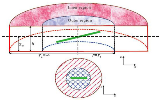
Figure 1.
Schematic diagram of highly deviated well in dual-porosity composite gas reservoir.
- (1)
- The reservoir is divided into two concentric radial composite regions. The physical properties of inner region are better than that of outer region.
- (2)
- Boundaries at top and bottom are closed both for inner and outer region. There is no closed outer boundary in the radial direction for outer region.
- (3)
- Both inner and outer region are treated as dual-porosity systems, consisting of matrix pores and natural fractures. Transfer between matrix and fractures is pseudo-steady flow.
- (4)
- Stress sensitivity effect and threshold pressure gradient are taken into account both in inner and outer region.
- (5)
- Permeabilities in both two regions are anisotropic in horizontal and vertical directions.
- (6)
- The effects of capillary force and gravity are neglected.
3. Mathematical Model
3.1. Basic Continuous Point Source Solution
Because of the effects of stress sensitivity and threshold pressure gradient, there are more complex nonlinear terms in governing equations of dual-porosity composite gas reservoir. Direct analytical solutions are not possible. A series of transformations are required so that they could be solved linearly. Based on the definition of pseudo pressure and dimensionless quantities, the dimensionless governing can be obtained and expressed by (see Appendix A):
Inner region
Natural fractures:
Matrix:
Outer region
Natural fractures:
Matrix:
Because the value of is small, , the following relationships exist according to perturbation method [27]:
Based on the corresponding initial conditions, boundary conditions and the zeroth order perturbation solution of Equations (5)–(7), governing equations and definite conditions in Laplace domain are:
Inner region
Outer region
Boundary conditions
Interface boundary conditions
To eliminate the variable zD in governing equations, Fourier transform of x0 with respect to zD is defined as:
and the inverse Fourier transform as:
where
According to properties of Fourier transform, the first four terms of governing Equations (8) and (9) can be transformed into:
So governing equations and definite conditions Equations (8)–(15) can be simplified.
where
when , the third terms of Equations (22) and (23) are equal to 0, which means that the effect of threshold pressure gradient is ignored. Equations (22) and (23) are Bessel equations of order 0. The general solutions of governing equations can be expressed by:
when , Equations (22) and (23) are inhomogeneous second order partial differential equations. The general solutions of governing equations can be expressed by:
where
Substituting Equations (31) and (32) into Equations (24)–(27), the 4 undetermined coefficients ,,, can be obtained.
where
Then the coefficients were substituted into the general solutions of the governing equations, and the inverse Fourier transform was used to obtain the basic continuous point source solution:
where
3.2. Establishment of Mathematical Model
According to the assumptions of physical model, the flow rate of a highly deviated well is evenly distributed along the well. Based on the principle of superposition for point source solution, the pressure of deviated well can be obtained by integration of Equation (42) along the wellbore.
where
The uniform flux source solution can be transformed into infinite-conductivity source solution, based on the research of Cinco [28]. Through the utilization of equivalent pressure point coordinates Equations (47)–(49), the pressure response of infinite-conductivity deviated well can be obtained.
To improve the model, the effects of skin and wellbore storage are taken into account based on Duhamel principle [29].
3.3. Solution of Mathematical Model
The detail solution process for this model can be divided into the following steps: (1) Calculate the dimensionless quantities need for Equation (45). (2) Compute uniform flux source solution in Laplace space for different s. Transform the uniform flux source solution into infinite-conductivity source solution with the utilization of equivalent pressure point coordinates. (3) Calculate the bottom hole pressure with consideration of the effects of skin and wellbore storage. (4) Apply Stehfest numerical inversion [30,31,32] and substitution relationship Equation (A21) to obtain pseudo-pressure of highly deviated well in real space. Then go back to step (2) and repeat above steps for different time steps. (5) With the corresponding relationship between pressure and time, the derivative of pressure can be obtained. Furthermore, the log-log typical curves can also be drawn.
4. Results and Discussion
4.1. Validation
Although there have been some studies on the composite model for highly deviated wells, they have not considered the effects of stress sensitivity and threshold pressure gradient in a dual medium gas reservoir. Because there is no direct reference to verify the model proposed in this paper, a simplified model of highly deviated well considering only one region is used to compare with other model [23]. The basic parameters used for validation are listed in Table 1.

Table 1.
Formation, fluid and wellbore parameters for verification.
The proposed composite model can be simplified to one region (when M21 = 1) dual medium model without considering threshold pressure gradient and stress sensitivity (when γmD = 0 and λmD = 0). Comparison of log-log transient pseudo-pressure curves between simplified model in this paper and the model of Wang et al. is shown in Figure 2. There is a great agreement both for pseudo-pressure curves and derivative curves, which indicates that the simplified model is valid.
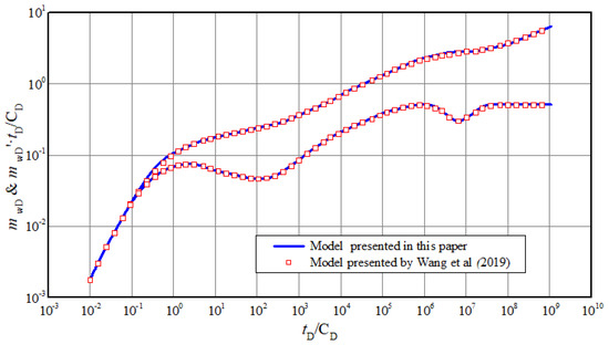
Figure 2.
Comparison of transient pressure curves with results of Wang et al.’s model.
4.2. Pressure Transient Characteristics and Flow Regimes
Based on a mathematical model and solving method, the response of wellbore pseudo-pressure and its derivative over time is obtained and drawn in log-log coordinate system as shown in Figure 3. It can be observed that the flow of gas can be divided into eight flow regimes.
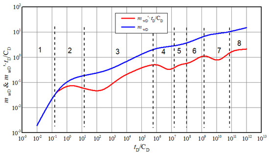
Figure 3.
Typical log-log curves of highly deviated well in composite carbonate gas reservoir.
- (1)
- Wellbore storage period. The pseudo-pressure and pseudo-pressure derivative are straight lines with 45°.
- (2)
- Transient flow under skin effect. The pseudo pressure derivative curve rises to a high point to form a “Hump” and then drops immediately.
- (3)
- Inclination angle dominated flow. The pseudo pressure derivative curve is mainly affected by the inclination angle of highly deviated well.
- (4)
- Interporosity flow between matrix and fractures in inner region. There is a “dip” on derivative curve which reflects the characteristics of dual medium.
- (5)
- Pseudo-radial flow in inner region. The pseudo-pressure derivative curve is an approximate horizontal line with value 0.5.
- (6)
- Transient flow between inner and outer region. The pseudo pressure derivative curve is an ascending line due to the poor physical properties of the outer region.
- (7)
- Interporosity flow between matrix and fractures in outer region. Similarly, “dip” appears.
- (8)
- Pseudo-radial flow of system. The pseudo pressure derivative curve is a rising line instead of horizontal line due to the non-Darcy effect.
4.3. Sensitivity Analysis of Pressure Responses
Figure 4 shows the effect of permeability modulus on typical curves. It can be seen that the pseudo-pressure and pseudo-pressure derivative curves rise with permeability modulus increasing. The pressure performance is influenced by permeability modulus from the 4th stage (interporosity flow between matrix and fractures in inner region) onwards. Furthermore, with the progress of production, the difference brought by permeability modulus gradually increases. During the third stage, the flow is approximate to linear flow of fracture around highly deviated well. When the gas in the fractures is produced, the pressure difference between the matrix and the fractures will inevitably result in the pressure drop of matrix. Then the stress sensitivity effect gradually begins to show. At this time, the effective permeability of gas reservoir decreases with pressure drop. So, the greater the permeability modulus, the higher the pseudo-pressure and pseudo-pressure derivative curve rise. Based on the above analysis, when the measured log-log pressure curves rise from the 4th stage and pressure derivative is not 0.5 in pseudo-radial flow of system, it can be inferred that non-Darcy flow exists.
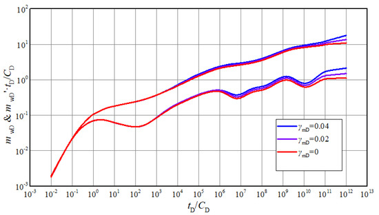
Figure 4.
The effect of permeability modulus on transient pseudo-pressure and derivative curves.
The typical curves for different threshold pressure gradient exhibit similar characteristics with the curves affected by permeability modulus as shown in Figure 5. Starting from 4th stage, gas in matrix has to overcome a certain pressure gradient to flow, meaning that a greater pressure difference is necessary to reach equivalent production. If there is also a stress sensitivity effect, the presence of the threshold pressure gradient will exacerbate the pressure drop and lead to greater permeability damage. So, the bigger the threshold pressure gradient is, the more typical curves become upturned. In the actual well test interpretation, if the pressure derivative of last stage is more than 0.5 and curves become upturned from 4th stage, it could be inferred that non-Darcy flow exists.
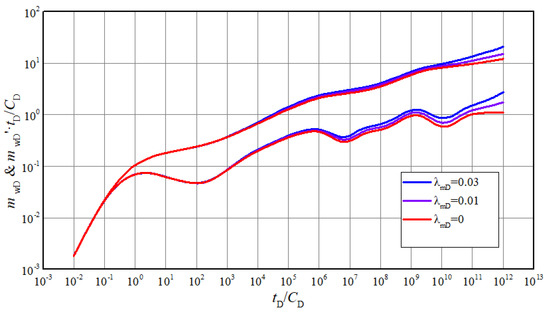
Figure 5.
The effect of threshold pressure gradient on transient pseudo-pressure and derivative curves.
For low-permeability gas reservoir, both threshold pressure gradient and stress sensitivity will result in non-Darcy flow. As shown in Figure 6, the blue curves are pressure responses considering the combination of threshold pressure gradient and stress sensitivity, marked as non-Darcy flow. In contrast, these effects are not taken into account for red curves. The values of other parameters are the same as above, except threshold pressure gradient and permeability modulus ( for non-Darcy flow and for Darcy flow). It could be found that the typical curves of Darcy flow are lower than non-Darcy flow. The red pseudo-pressure derivative curve is almost a horizontal line in stage 8, meaning that it is radial flow. So, it is a typical characteristic to determine whether there is a non-Darcy phenomenon.
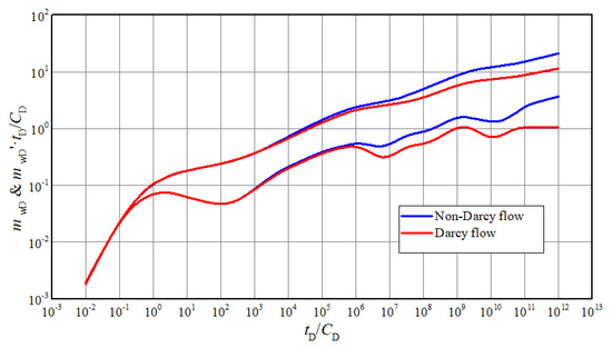
Figure 6.
Comparison of typical curves between non-Darcy flow and Darcy flow.
Figure 7 shows the influence of mobility ratio on the typical well test curves. It mainly occurs from stage 6 to stage 8. In general, the lower the mobility ratio is, the higher the curves are. However, different mobility ratios represent different physical properties in inner and outer regions. If the mobility ratio is equal to 1, the model can be simplified to triple medium reservoir with only one region. For Darcy flow, the two “dip” will be approximately in the same horizontal position. However, the latter “dip” in stage 7 will higher that the former in stage 5, with consideration of threshold pressure gradient and stress sensitivity effect. When the mobility ratio of outer to inner regions is greater than 1, it means that the flow capacity of outer region is better than the one of inner region. When the mobility ratio is less than 1, the physical properties of outer region are worse than that of the internal region. In this case, the gas flow in outer region needs a larger pressure difference, so the pseudo-pressure and pseudo-pressure derivative curves will rise. In well test interpretation, if the measured curve in stage 7 is lower than stage 5, it could be inferred that the flow capacity of outer region is better than the one of inner region, which means the acidification effect is poor.
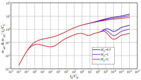
Figure 7.
The effect of mobility ratio on transient pseudo-pressure and derivative curves.
Figure 8 and Figure 9 show the effects of inter-porosity flow coefficient and storability ratio on curves, respectively. The two parameters mainly influence the curves characteristics of the 4th stage. The dip appears earlier with the increasing of inter-porosity flow coefficient. The positions of pseudo-pressure and derivative curves lower and the dips become deeper with the decreasing of storability ratio. Similar to inner region, the two parameters of outer region will have the same function on curves in 7th stage. In actual interpretation, the depth of dip in the measured curves can be used to identify storage capacity of matrix and fractures. The occurrence time of dip in measured curves can be used to identify the ability of inter-porosity flow.
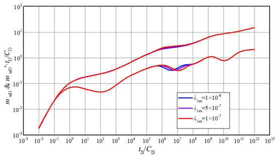
Figure 8.
The effect of inter-porosity flow coefficient of inner region on typical curves.
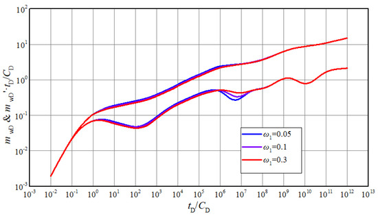
Figure 9.
The effect of storability ratio of inner region on typical curves.
It can be seen from Figure 10 that stage 6 appears earlier with the decreasing of the radius of inner region. In this case, mobility ratio is less than 1, that is, flow capacity of inner region is better than the one of outer region. The larger the inner region is, the better the acidification effect will be, so the pressure and derivative curves will be lower. If radius of the inner region is small to a certain extent, the pseudo-radial flow of the inner region will disappear. Due to the small area of the inner region, gas is supplied from the outer region before the radial flow of inner region is formed. The radius of the inner zone determines the time when the gas in the outer region begins to flow into the inner zone. In an actual interpretation, the longer pseudo-radial flow of the inner region lasts, the larger the inner region. If the mobility ratio is less than 1, it could be inferred that the acidification effect is great.
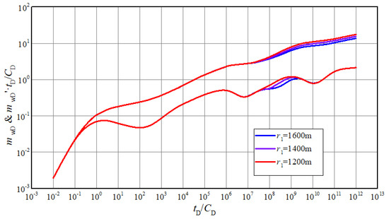
Figure 10.
The effect of radius of inner region on transient pseudo-pressure and derivative curves.
5. Conclusions
The research investigated the pressure performance of a highly deviated well in a carbonate gas reservoir. A dual-porosity composite model was established with a consideration of the effects of stress sensitivity and threshold pressure gradient. A semi-analytical method was used to deal with the nonlinearity of flow equation. The solution of pressure and typical log-log curves with eight flow regimes were obtained. Furthermore, the effects of relevant factors on log-log pressure curves were studied to guide the interpretation of actual well test. The main conclusion are as follows:
- (1)
- The validity of the proposed model was verified by matching it with another analytical model. It shows that the dual-porosity composite model can be used for well test interpretation of highly deviated well in carbonate gas reservoir.
- (2)
- The presence of non-Darcy flow effect can be diagnosed from the log-log curve. The pseudo-pressure derivative curve is a rising line instead of horizontal line due to the non-Darcy effect in pseudo-radial flow of system.
- (3)
- Permeability modulus and threshold pressure gradient will influence the characteristics of log-log curves from 4th flow stage on. The derivative curve will become upturned with the effects of them, and the greater the value, the higher curve rise.
- (4)
- The depth of dip in the measured curves can be used to identify storage capacity of matrix and fractures. The occurrence time of dip in measured curves can be used to identify the ability of inter-porosity flow.
- (5)
- In actual interpretation, the longer the pseudo-radial flow of inner region lasts, the larger the inner region. If the mobility ratio is less than 1, it could be inferred that the acidification effect is great.
- (6)
- Compared with other models, the model presented in this paper is more suitable for carbonate gas reservoir. With its high efficiency and simplicity, this proposed model will serve as a useful tool to evaluate the pressure performance for highly deviated well in carbonate gas reservoirs.
Author Contributions
Conceptualization, L.Z. and Q.Z.; methodology, Q.L.; software, Q.Z.; validation, Y.J. and Q.L.; investigation, L.Z.; resources, L.Z. and Y.J.; writing—original draft preparation, Q.Z.; writing—review and editing, Q.L.; supervision, L.Z. All authors have read and agreed to the published version of the manuscript.
Funding
This research received no external funding.
Conflicts of Interest
The authors declare no conflict of interest.
Nomenclature
| CD | Dimensionless wellbore storage coefficient, dimensionless |
| S | Skin factor, dimensionless |
| s | Laplace transform parameter, dimensionless |
| Z | Real-gas compressibility factor, dimensionless |
| t | Time, s |
| qex | Matrix-to-fractures inter-porosity flow, m3/s |
| qsc | Production rate at surface conditions, m3/s |
| qscins | Production rate of continuous column source at surface conditions, m3/s |
| cft | Compressibility of gas and rock in fracture system, Pa−1 |
| cmt | Compressibility of gas and rock in matrix system, Pa−1 |
| r | Radial distance in natural fracture system, m |
| rw | Wellbore radius, m |
| pm | Pressure of matrix, Pa |
| pf | Pressure of natural fracture, Pa |
| pi | Initial reservoir pressure, Pa |
| mm | Pseudo-pressure of matrix system, Pa |
| mf | Pseudo-pressure of fracture system, Pa |
| M21 | Mobility ratio of outer region to inner region, fraction |
| μ | Gas viscosity, Pa·s |
| kfh | Horizontal permeability of natural fracture, m2 |
| kfv | Vertical permeability of natural fracture, m2 |
| km | Permeability of matrix, m2 |
| ρ | Gas density, kg/m3 |
| h | Reservoir thickness, m |
| Porosity of natural fracture, fraction | |
| Porosity of matrix, fraction | |
| L | Characteristic length, m |
| hw | Length of highly deviated well, m |
| θ | Deviation angle, ° |
| x | Pseudo pressure considering permeability modulus, Pa |
| ω | Storability ratio, dimensionless |
| γ | Permeability modulus, 1/Pa |
| λex | Inter-porosity flow coefficient, dimensionless |
| λm | Threshold pressure gradient, Pa/m |
| α | Shape factors, dimensionless |
| zw | Coordinates of source, m |
| z | z-coordinates of gas reservoir, m |
| Subscript | |
| i | Initial state |
| m | Matrix |
| f | Natural fracture |
| sc | Standard state |
| w | Wellbore/source |
| D | Dimensionless |
| 1 | Inner region |
| 2 | Outer region |
| Superscript | |
| ̅ | Laplace transform |
| ~ | Fourier transform |
Appendix A. Derivation of Continuous Point Source Equations
Both inner and outer region are treated as dual-porosity systems, consisting of matrix pores and natural fractures. By substituting equation of state and transport equation coupled multiple mechanisms into the continuity equation, the governing equations for composite carbonate gas reservoir can be obtained.
Inner region
Natural fractures:
Matrix:
Outer region
Natural fractures:
Matrix:
Interporosity flow between matrix and fractures is pseudo-steady. So, the exchange of fluid can be expressed by:
Initial conditions
The initial pressure of gas reservoir is uniform and equal to original formation pressure pi.
Boundary conditions
There is a continuous column source at (xw, yw, zw). The inner boundary condition can be written as:
The outer boundary is laterally infinite.
The top and bottom of gas reservoir are closed, which can be given by:
Interface boundary conditions
Pressure and flow rate are equal at the interface between the inner and outer zones.
The governing equations and definite conditions of composite dual-porosity carbonate gas reservoir are the combination of Equations (A1)–(A13). The above equations are still highly nonlinear. Based on pseudo-pressure Equation (A14), define the expression of permeability modulus Equation (A15) and threshold pressure gradient Equation (A16) under pseudo pressure.
It is assumed that both viscosity and compressibility are constant values in the original state. According to the introduction of permeability modulus and threshold pressure gradient under pseudo-pressure, the governing Equations (A1)–(A4) can be rewritten in pseudo-pressure form.
Inner region
Natural fractures:
Matrix:
Outer region
Natural fractures:
Matrix:
Governing equations are very complicated and has quadratic terms of quasi-pressure partial derivatives. To further linearize the equations, dimensionless variables listed in Table A1 and pseudo pressure transformation based on Equation (A21) are substituted into governing equations.
Table A1.
Definition of dimensionless variables.
Table A1.
Definition of dimensionless variables.
| Dimensionless Variables | Expression | Dimensionless Variables | Expression |
|---|---|---|---|
| Dimensionless wellbore radius | Dimensionless radius | ||
| Dimensionless distance of x coordinate | Dimensionless distance of y coordinate | ||
| Dimensionless vertical distance of mid-perforation | Dimensionless vertical distance | ||
| Dimensionless permeability modulus | Dimensionless pseudo threshold pressure gradient | ||
| Dimensionless deviation angle | Dimensionless time | ||
| Dimensionless pseudo-pressure of matrix system | Dimensionless length of highly deviated well | ||
| Dimensionless pseudo-pressure of fracture system | Dimensionless wellbore storage coefficient | ||
| Mobility ratio between outer and inner regions | Interporosity flow coefficient between fractures and matrix | ||
| Dimensionless pseudo-pressure | Storativity ratio of matrix system |
Then the governing equations of continuous point source are simplified to:
Inner region
Natural fractures:
Matrix:
Outer region
Natural fractures:
Matrix:
References
- Yue, P.; Xie, Z.; Huang, S.; Liu, H.; Liang, S.; Chen, X. The application of N2 huff and puff for IOR in fracture-vuggy carbonate reservoir. Fuel 2018, 234, 1507–1517. [Google Scholar] [CrossRef]
- Wang, L.; Yang, S.; Liu, Y.; Xu, W.; Deng, H.; Meng, Z.; Han, W.; Qian, K. Experiments on gas supply capability of commingled production in a fracture-cavity carbonate gas reservoir. Pet. Explor. Dev. 2017, 44, 824–833. [Google Scholar]
- Wei, G.; Yang, W.; Du, J.; Xu, C.; Zou, C.; Xie, W.; Wu, S.; Zeng, F. Tectonic features of Gaoshiti-Moxi paleo-uplift and its controls on the formation of a giant gas field, Sichuan Basin, SW China. Pet. Explor. Dev. 2015, 42, 283–292. [Google Scholar]
- Zhou, Z.; Wang, X.; Yin, G.; Yuan, S.; Zeng, S. Characteristics and genesis of the (Sinian) Dengying Formation reservoir in Central Sichuan, China. J. Nat. Gas Sci. Eng. 2016, 29, 311–321. [Google Scholar] [CrossRef]
- Zhao, L.; Chen, Y.; Ning, Z.; Fan, Z.; Wu, X.; Liu, L.; Chen, X. Stress sensitive experiments for abnormal overpressure carbonate reservoirs: A case from the Kenkiyak low-permeability fractured-porous oilfield in the littoral Caspian Basin. Pet. Explor. Dev. 2013, 40, 194–200. [Google Scholar]
- Warren, J.E.; Root, P.J. The behavior of naturally fractured reservoirs. Soc. Pet. Eng. J. 1963, 3, 245–255. [Google Scholar] [CrossRef]
- Abdassah, D.; Ershaghi, I. Triple-porosity systems for representing naturally fractured reservoirs. SPE Form. Eval. 1986, 1, 113–127. [Google Scholar] [CrossRef]
- Camacho-Velazquez, R.; Vasquez-Cruz, M.; Castrejon-Aivar, R.; Arana-Ortiz, V. Pressure transient and decline curve behaviors in naturally fractured vuggy carbonate reservoirs. In Proceedings of the SPE Annual Technical Conference and Exhibition, San Antonio, TX, USA, 29 September–2 October 2020. [Google Scholar]
- Al-Ghamdi, A.; Ershaghi, I. Pressure transient analysis of dually fractured reservoirs. SPE J. 1996, 1, 93–100. [Google Scholar] [CrossRef]
- Li, Z.; Duan, Y.; Wei, M.; Peng, Y.; Chen, Q. Pressure performance of interlaced fracture networks in shale gas reservoirs with consideration of induced fractures. J. Pet. Sci. Eng. 2019, 178, 294–310. [Google Scholar] [CrossRef]
- Chen, P.; Wang, X.; Liu, H.; Huang, Y.; Chen, S.; Zhang, H. A pressure-transient model for a fractured-vuggy carbonate reservoir with large-scale cave. Geosyst. Eng. 2016, 19, 69–76. [Google Scholar] [CrossRef]
- He, J.; Killough, J.E.; Fadlelmula, F.; Mohamed, M.; Fraim, M. A unified finite difference model for the simulation of transient flow in naturally fractured carbonate karst reservoirs. In Proceedings of the SPE Reservoir Simulation Symposium, Houston, TX, USA, 23–25 February 2015. [Google Scholar]
- Agada, S.; Chen, F.; Geiger, S.; Toigulova, G.; Agar, S.; Shekhar, R.; Benson, G.; Hehmeyer, O.; Amour, F.; Mutti, M. Numerical simulation of fluid-flow processes in a 3D high-resolution carbonate reservoir analogue. Pet. Geosci. 2014, 20, 125–142. [Google Scholar]
- Li, L.; Huang, J.; Luo, C.; Du, F.; Liu, Y. Study on Productivity Numerical Simulation of Highly Deviated and Fractured Wells in Deep Oil and Gas Reservoirs. In Proceedings of the MATEC Web of Conferences; EDP Sciences: Société Chimique de France, France, 2016; p. 07003. [Google Scholar]
- Medeiros, F.; Ozkan, E.; Kazemi, H. A semianalytical, pressure-transient model for horizontal and multilateral wells in composite, layered, and compartmentalized reservoirs. In Proceedings of the SPE Annual Technical Conference and Exhibition, San Antonio, TX, USA, 24–27 September 2006. [Google Scholar]
- Olarewaju, J.S.; Lee, W.J. An analytical model for composite reservoirs produced at either constant bottomhole pressure or constant rate. In Proceedings of the SPE Annual Technical Conference and Exhibition, Dallas, TX, USA, 27–30 September 1987. [Google Scholar]
- Olarewaju, J.S.; Lee, W.J. A comprehensive application of a composite reservoir model to pressure transient analysis. In Proceedings of the SPE California Regional Meeting, Ventura, CA, USA, 8–10 April 1987. [Google Scholar]
- Wei, M.; Duan, Y.; Dong, M.; Fang, Q. Blasingame decline type curves with material balance pseudo-time modified for multi-fractured horizontal wells in shale gas reservoirs. J. Nat. Gas Sci. Eng. 2016, 31, 340–350. [Google Scholar] [CrossRef]
- Zeng, H.; Fan, D.; Yao, J.; Sun, H. Pressure and rate transient analysis of composite shale gas reservoirs considering multiple mechanisms. J. Nat. Gas Sci. Eng. 2015, 27, 914–925. [Google Scholar] [CrossRef]
- Zhang, L.; Guo, J.; Liu, Q. A well test model for stress-sensitive and heterogeneous reservoirs with non-uniform thicknesses. Pet. Sci. 2010, 7, 524–529. [Google Scholar] [CrossRef][Green Version]
- Yang, Y.; Liu, Z.; Sun, Z.; An, S.; Zhang, W.; Liu, P.; Yao, J.; Ma, J. Research on stress sensitivity of fractured carbonate reservoirs based on CT technology. Energies 2017, 10, 1833. [Google Scholar] [CrossRef]
- Wu, H.; Li, F.; Liu, J.; Chen, J.; Lv, X.; Hu, W. An experimental study on low-velocity nonlinear flow in vuggy carbonate reservoirs. Geosyst. Eng. 2016, 19, 151–157. [Google Scholar] [CrossRef]
- Wang, K.; Wang, L.; Adenutsi, C.D.; Li, Z.; Yang, S.; Zhang, L.; Wang, L.; Wen, P.H. Analysis of Gas Flow Behavior for Highly Deviated Wells in Naturally Fractured-Vuggy Carbonate Gas Reservoirs. Math. Probl. Eng. 2019, 2019, 6919176. [Google Scholar] [CrossRef]
- Wang, Y.; Yi, X. Flow modeling of well test analysis for a multiple-fractured horizontal well in triple media carbonate reservoir. Int. J. Nonlinear Sci. Numer. Simul. 2018, 19, 439–457. [Google Scholar] [CrossRef]
- Wei, M.; Duan, Y.; Dong, M.; Fang, Q.; Dejam, M. Transient production decline behavior analysis for a multi-fractured horizontal well with discrete fracture networks in shale gas reservoirs. J. Porous Media 2019, 22, 343–361. [Google Scholar] [CrossRef]
- Meng, F.; Lei, Q.; He, D.; Yan, H.; Jia, A.; Deng, H.; Xu, W. Production performance analysis for deviated wells in composite carbonate gas reservoirs. J. Nat. Gas Sci. Eng. 2018, 56, 333–343. [Google Scholar] [CrossRef]
- Wang, H. Performance of multiple fractured horizontal wells in shale gas reservoirs with consideration of multiple mechanisms. J. Hydrol. 2014, 510, 299–312. [Google Scholar] [CrossRef]
- Cinco, H.; Miller, F.G.; Ramey, H.J., Jr. Unsteady-state pressure distribution created by a directionally drilled well. J. Pet. Technol. 1975, 27, 1392–1400. [Google Scholar] [CrossRef]
- Van Everdingen, A.F. The Skin Effect and Its Influence on the Productive Capacity of a Well. Trance AIME 1953, 198, 171–176. [Google Scholar] [CrossRef]
- Peng, Y.; Zhao, J.; Sepehrnoori, K.; Li, Y.; Yu, W.; Zeng, J. Study of the Heat Transfer in the Wellbore During Acid/Hydraulic Fracturing Using a Semianalytical Transient Model. SPE J. 2019, 24, 877–890. [Google Scholar] [CrossRef]
- Peng, Y.; Zhao, J.; Sepehrnoori, K.; Li, Z.; Xu, F. Study of delayed creep fracture initiation and propagation based on semi-analytical fractional model. Appl. Math. Model. 2019, 72, 700–715. [Google Scholar] [CrossRef]
- Peng, Y.; Zhao, J.; Sepehrnoori, K.; Li, Z. Fractional model for simulating the viscoelastic behavior of artificial fracture in shale gas. Eng. Fract. Mech. 2020, 228, 106892. [Google Scholar] [CrossRef]


Publisher’s Note: MDPI stays neutral with regard to jurisdictional claims in published maps and institutional affiliations. |
© 2020 by the authors. Licensee MDPI, Basel, Switzerland. This article is an open access article distributed under the terms and conditions of the Creative Commons Attribution (CC BY) license (http://creativecommons.org/licenses/by/4.0/).