Estimation for Battery State of Charge Based on Temperature Effect and Fractional Extended Kalman Filter

Abstract

The electric vehicle has become an important development direction of the automobile industry, and the lithium-ion power battery is the main energy source of electric vehicles. The accuracy of state of charge (SOC) estimation directly affects the performance of the vehicle. In this paper, the first order fractional equivalent circuit model of a lithium iron phosphate battery was established. Battery capacity tests with different charging and discharging rates and open circuit voltage tests were carried out under different ambient temperatures. The conversion coefficient of charging and discharging capacity and the simplified open circuit voltage model considering the hysteresis characteristics of the battery were proposed. The parameters of the first order fractional equivalent circuit model were identified by using a particle swarm optimization algorithm with dynamic inertia weight. Finally, the recursive formula of a fractional extended Kalman filter was derived, and the battery SOC was estimated under continuous Dynamic Stress Test (DST) conditions. The results show that the estimation method has high accuracy and strong robustness.

1. Introduction

With the decrease in non-renewable energy and the turbulence of the global energy situation, the development of green energy has become an important theme of the global automobile industry [1,2]. In the past decade, electric vehicles have shown a rapid development trend, and ownership has increased year by year. However, electric vehicles still have shortcomings, such as short driving range and long charging time, so research on key technologies of electric vehicles is urgent. The estimation of battery state of charge (SOC) is one of the key technologies of electric vehicles [3]. The accuracy directly affects the whole vehicle energy management control system and regenerative braking control system [4], and then affects the driving range of the vehicle. At the same time, the battery SOC is also an important parameter in the battery management system, which can provide a basis for the battery management and maintenance system to prevent the battery from over charging or discharging, which will lead to the decrease in battery life and potential safety hazards. However, it is inconvenient to measure the battery SOC directly by instruments, so it can only be estimated by relevant parameters. Affected by many factors such as temperature, charging–discharging rate, noise and so on, which makes the estimation quite difficult. Therefore, research on the estimation of SOC has been carried out in the past ten years [5,6,7,8,9,10,11,12,13,14].

At present, the SOC estimation methods which are not based on the battery model are relatively simple, mainly including the ampere hour integration method, the open circuit voltage (OCV) method and the internal resistance method, but those methods generally have low accuracy, poor anti-noise ability and other shortcomings [15,16]. With the development of neural networks, fuzzy algorithms, support vector machines and other intelligent algorithms [9,10,11], SOC estimation methods based on a black-box battery model have emerged [17,18,19,20]. In reference [21], the neural network and unscented Kalman filter (UKF) were used in series to estimate SOC, and the Root Mean Square (RMS) errors of the SOC estimation were within 2.5% and maximum errors were within 3.5% for different temperatures. In reference [22], the voltage, current and temperature of the battery were fuzzed, and then the fuzzy rule base was established according to the experience, so the battery SOC was obtained by defuzzification. In reference [23], a nonlinear fuzzy support vector machine algorithm was proposed by combining a support vector machine and fuzzy algorithm, which improved the accuracy of SOC estimation. However, an SOC estimation method based on a black-box model usually requires an off-line database, and the process of sample training has a large amount of calculations, which is prone to over fitting and falling into local optimization, so it is difficult to apply in engineering.

The idea of an SOC estimation method based on a state space model is based on the equivalent circuit model, taking the measured current and voltage as the observed input to estimate the current SOC value of the battery [15], which is a more general and in-depth SOC estimation method at present. Therefore, the design of an equivalent circuit model and observer is the key content of this method [12]. The equivalent circuit model of the battery is mainly divided into an integer order model and a fractional order model [24]. The integer order model needs a higher order to simulate the battery terminal voltage characteristics more accurately, which will greatly increase the amount of calculations, while the fractional order model can use less order to achieve higher accuracy, which has been widely investigated. In reference [25], based on the PNGV model, the fractional element was used to replace the capacitance on the main circuit and the capacitance on the (Resistor-Capacitance) RC ring, and the accuracy of the fractional order model in the low frequency region was verified. In reference [26], the equivalent circuit model of fractional order was obtained by connecting the internal resistance and fractional order elements in series, and the voltage characteristics of fractional elements under different orders were studied. In reference [27], the fractional equivalent circuit model was established by using a constant phase element (CPE) and variable order Warburg elements, and compared with the integer model in first order. In reference [28], based on the RC integral model in first order, the equivalent circuit model in fractional order was established by replacing the capacitor with a fractional capacitor element, which verified the accuracy of the model. However, most of the fractional order models usually study the parameters at a single temperature, without considering the change of the parameters of the equivalent circuit model when the ambient temperature changes, so the model usually has low practicability. Moreover, most of the literature has little research on the hysteresis characteristics of open circuit voltage in a power battery, especially the lithium iron phosphate battery. When the battery state changes frequently, if not considering the hysteresis characteristics of the open circuit voltage, the error of the model output voltage will be extended, and the accuracy of the model will decrease. The most widely used observer is the extended Kalman filter (EKF) which has nonlinear estimation ability to estimate the SOC of a battery [25], but, for integer order models, the accuracy is poor. So, an adaptive extended Kalman filter (AEKF) [29,30,31], volume Kalman filtering (CKF) [32], unscented Kalman filter (UKF) [8,33], dual EKF [34] and various improved forms based on the Kalman filter [5,35] are used to estimate SOC. For the fractional order model, using EKF and UKF can achieve ideal results because of high accuracy of terminal voltage and the memory of data.

In this paper, the influence of temperature and hysteresis characteristics of open circuit voltage on the fractional order model was considered, and the SOC estimation of a battery was studied by using the extended Kalman filter. The structure of this paper is as follows. In the second section, based on the definition of Grunwald–Letnikov (G-L) type calculus, the first order fractional equivalent circuit model was established by modifying the first order integer model. In the third section, the characteristics of battery capacity and open circuit voltage at different temperatures were studied, and a simplified open circuit voltage model considering hysteresis characteristics was established. Then, in the fourth section, the particle swarm optimization method was used to identify the parameters of a fractional equivalent circuit model at different temperatures. In the fifth section, SOC was estimated by using a fractional extended Kalman filter, and the validity and reliability of the proposed method were verified. The structure of the article is shown in Figure 1.

2. Fractional Order Model

2.1. Fractional Order Theory

The essence of fractional order is the extension from integral order calculus to non-integral order calculus. At present, fractional order calculus is widely used in viscoelastic mechanics, soft matter mechanics and other disciplines, and it also has preliminary application in the estimation of battery SOC for new energy vehicles. The literature [36] shows the rationality of the application of fractional calculus theory used in a battery. The accuracy of the model terminal voltage can be improved by establishing the battery equivalent circuit model based on the fractional calculus theory.

At present, the definition of fractional calculus mainly includes G-L type, Riemann–Liouville (R-L) type, Caputo type and Weyl type. The equivalent circuit model of a battery based on G-L type is most widely used, which is generalized by the difference recurrence formula of an integer order derivative. When the fractional order α > 0, the definition is as follows:

$${}_a{}^{GL}D_t^{\alpha }f(t)=\underset{h\to 0}{\lim }{f}_h^{(\alpha )}(t)\stackrel{\mathrm{def}}{=}\underset{h\to 0^{+},nh=t-a}{\lim }{h}^{-\alpha }{\displaystyle \sum _{i=0}^n\left[\begin{array}{c}-\alpha \\ i\end{array}\right]}f(t-ih)$$

(1)

$$\left[\begin{array}{c}-\alpha \\ i\end{array}\right]=\{\begin{array}{c}\frac{(-\alpha )(-\alpha +1)(-\alpha +2)\cdots (-\alpha +i-1)}{i!},i\ne 0\\ \hspace{1em}\hspace{1em}\hspace{1em}\hspace{1em}\hspace{1em}1,\hspace{1em}\hspace{1em}\hspace{1em}\hspace{1em}\hspace{1em}i=1\end{array}$$

(2)

In the formula, a is the lower limit of the interval; t is the upper limit of the interval; h is the sampling interval and n = t/h. In the following text, ${}_a{}^{GL}D_t^{\alpha }x(t)$ is expressed as $D_{}^{\alpha }x(t)$ for ease of writing.

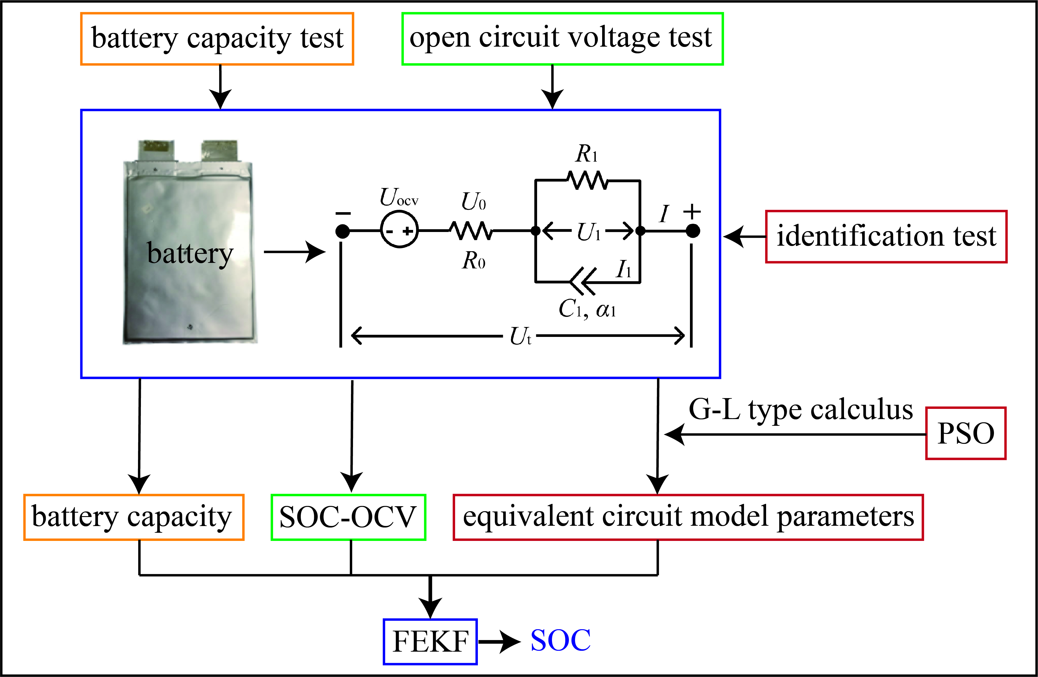
2.2. Fractional Equivalent Circuit Model

At present, the commonly used integer order equivalent circuit models are the Rint model, Thevenin model and PNGV model, while the fractional order equivalent circuit model is mostly obtained by modifying the integral order equivalent circuit model. In this paper, considering that the fractional order has data memory characteristics, resulting in larger amounts of calculations than the integer order, in order to reduce the difficulty of parameter identification, the fractional equivalent circuit model is obtained by replacing the capacitance in Thevenin model with fractional CPE, as shown in Figure 2. CPE is a constant phase component; its order varies from 0–1. It is a fractional order circuit element between resistance and ideal capacitance. When the order is 1, it is equivalent to ideal capacitance, when the order is 0, it is equivalent to ideal resistance. Its mathematical formula depends on the choice of fractional order type and, in this paper, the fractional type of CPE is the G-L type defined above and its value is obtained through a parameter identification test and parameter identification method under different conditions.

U_ocv is the voltage source, which can be used to simulate the open circuit voltage of the battery. It is one of the important parameters affecting the SOC estimation of the power battery, and also the non-linear part for the equivalent circuit model. It will be obtained from the data measured by the open circuit voltage test; U₀ is the terminal voltage of internal resistance; U₁ is the terminal voltage of the polarization ring; U_t is the battery terminal voltage, which is the output variable of the whole battery system; I is the total current, which is the input variable of the battery system, the current I is 0 when the battery is in a rest condition. In this paper, it is specified that when the battery is discharged, I is positive, and when charged, it is negative; I₁ is the current on CPE; R₀ is the internal resistance, which can reflect the voltage characteristics in the charging and discharging process; R₁ is the polarization internal resistance; the capacitance of CPE is C₁ and the order is α₁. The combination of R₁ and C₁ can reflect the polarization characteristics of the battery during charging, discharging and static processes.

According to the fractional order theory, the current on the CPE is:

$$I_1=C_1{D}^{{\alpha }_1}{U}_1$$

(3)

The voltage on the polarization ring is:

$$U_1=(I-C_1{D}^{{\alpha }_1}{U}_1)R_1$$

(4)

According to the Kirchhoff voltage principle, the battery terminal voltage is:

$$U_{\mathrm{t}}=U_{\mathrm{OCV}}-U_0-U_1$$

(5)

The calculation formula of the battery SOC is:

$$SOC(t)=SOC(0)-\frac{\eta }{Q_{\mathrm{N}}}{\displaystyle {\int }_0^{t}Idt}$$

(6)

where SOC(0) is the initial SOC value; η is the conversion coefficient of charging and discharging capacity; Q_N is the rated capacity of battery.

When h is a small positive number, Equation (1) can be approximately as follows:

$$D_{}^{\alpha }f(t)\approx h^{-\alpha }{\displaystyle \sum _{i=0}^n\left[\begin{array}{c}-\alpha \\ i\end{array}\right]}f(t-ih)$$

(7)

If $f(k-i)$ is substituted for $f(t-ih)$, Equation (7) can be rewritten as:

$$D_{}^{\alpha }f(k)=h^{-\alpha }{\displaystyle \sum _{i=0}^n\left[\begin{array}{c}-\alpha \\ i\end{array}\right]}f(k-i)$$

(8)

By discretizing Equation (4):

$$D^{{\alpha }_1}{U}_1(k+1)=-\frac{1}{C_1{R}_1}{U}_1(k)+\frac{1}{C_1}I(k)$$

(9)

In combination with the approximate fractional order calculation Equation (8), Equation (9) can further deduce:

$$h^{-{\alpha }_1}[U_1(k+1)+{\displaystyle \sum _{i=1}^n\left[\begin{array}{c}-{\alpha }_1\\ i\end{array}\right]}{U}_1(k+1-i)]=-\frac{1}{C_1{R}_1}{U}_1(k)+\frac{1}{C_1}I(k)$$

(10)

In summary, we can get:

$$U_1(k+1)=-\frac{h^{{\alpha }_1}}{C_1{R}_1}{U}_1(k)+\frac{h^{{\alpha }_1}}{C_1}I(k)-{\displaystyle \sum _{i=1}^n\left[\begin{array}{c}-{\alpha }_1\\ i\end{array}\right]}{U}_1(k+1-i)$$

(11)

If considering Gaussian white noise, the fractional discrete space state expression of the battery is as follows:

$$\{\begin{array}{l}x(k+1)=Ax(k)+BI(k)-M+\omega (k)\hfill \\ y(k)=h[x(k)]+DI(k)+\upsilon (k)\hfill \end{array}$$

(12)

where

• $x(k)={\left[SOC(k),U_1(k)\right]}^{\mathrm{T}}$; $y(k)=\left[U\mathrm{t}\right]$;
• $A=\mathrm{diag}\{1,-\frac{h^{{\alpha }_1}}{C_1{R}_1}\}$; $B={\left[\frac{-\eta h}{3600Q_N},\frac{h^{{\alpha }_1}}{C_1}\right]}^{\mathrm{T}}$; $M={\left[0,{\displaystyle \sum _{i=1}^n\left[\begin{array}{c}-{\alpha }_1\\ i\end{array}\right]}{U}_1(k+1-i)\right]}^{\mathrm{T}}$;
• $D(k)=\left[-R_0\right]$; $h[x(k)]=U_{\mathrm{OCV}}\left[SOC\right(k\left)\right]-U_1(k)$;

$\omega (k)$ is system noise, $\upsilon (k)$ is measurement noise, the variance of system noise is Q and the variance of measurement noise is R. M is the historical state including the polarization voltage up to the previous moment. The polarization voltage of the equivalent circuit model of the battery at the current moment is calculated by iteration, and then the battery terminal voltage is calculated by the observation equation.

3. Battery Characteristics under Different Influential Factors

In this paper, an A123 lithium iron phosphate battery was selected as the research object, and the battery capacity characteristics and open circuit voltage characteristics under the influence of different factors were studied. The rated capacity of the battery is 20 Ah, the rated voltage is 3.2 V, the charging cut-off voltage is 3.65 V and the discharging cut-off current is 0.5 A. In order to ensure the battery life, the discharging cut-off voltage is set to 2.5 V. The charging–discharging test bench was composed of a discharging–charging battery tester BT2016, upper computer, environmental chamber and multimeter HP34401A.

3.1. Characteristics of Battery Capacity

Battery capacity is the key factor affecting the accuracy of SOC estimation, but it is greatly affected by battery temperature and charging–discharging rate in actual use. Therefore, in order to improve the accuracy of SOC estimation, it is necessary to test the battery charging and discharging capacity under different temperatures and rates to obtain the conversion coefficient of charging–discharge capacity η and correct the battery SOC. In this paper, based on the Battery Test Manual for Electric Vehicles, η was calculated on the basis of capacity at 30 °C and a 3/C rate, as shown in Equation (13). The test scheme is shown in Figure 3. As an additional explanation, the capacity of the battery will decrease with an increase in the number of cycles. However, because the cycle life of the battery selected in this paper is more than 2000 times, the number of cycles consumed in the experiments of this paper is less than 150. The influence is small, so here is only a brief description, without considering the influence of cycle times on battery performance.

$$\eta =\{\begin{array}{r}\hfill {\eta }_{\mathrm{d}} =\frac{Q_{\mathrm{Nd}}}{Q_{T,C\mathrm{d}}}, I>0\\ \hfill {\eta }_{\mathrm{c}} =\frac{Q_{\mathrm{Nc}}}{Q_{T,C\mathrm{c}}}, I<0\end{array}$$

(13)

where η_d is the conversion coefficient of discharging capacity; η_c is the conversion coefficient of charging capacity; Q_T,Cd is the discharging capacity under different temperatures and discharging current; Q_T,Cc is the charging capacity under different temperatures and charging currents; Q_N is the rated capacity, which is 20.2 Ah according to the test; t is the environment temperature, T = 0, 5, 15, 25, 30, 35 °C; C_d is the discharging rate, C_d = C/3, C/2, 3C/4, C, 5C/4, 3C/2, 7C/4, 2C, 9C/4; C_c is the charging rate, C_c = C/3, C/2, 3C/4, C.

The curves of battery charging and discharging capacity at different temperatures and rates is shown are Figure 4 and Figure 5. The overall trend of charging and discharging capacity is the same. The capacity increases with an increase in the ambient temperature, and decreases with an increase in the current rate. The battery capacity in the cool environment is more sensitive to the ambient temperature and the change of capacity in the same temperature difference is greater than that in the high-temperature environment. The curve of battery discharging capacity tends to be flat or even slightly increased with an increase in the discharging rate, because the test object is a single battery without cooling equipment, which is in the state of natural convection in the environmental chamber, and the heat transfer coefficient is small. When the discharging rate is small, the temperature rise of the battery is small, and its own temperature is slightly higher than the ambient temperature, but with an increase in discharging rate, the temperature of the battery increases gradually. So, the difference of discharging capacity will decrease gradually, or the electric quantity will even rise. However, in the charging test, the maximum charging current is only C, and the temperature rise of the battery is not obvious at all ambient temperatures, so there is no such phenomenon. In the process of using the conversion coefficient of capacity in the later simulation calculation, because there are two independent variables of ambient temperature and rate, the conversion coefficient out of the test condition is obtained by a two-dimensional quadratic spline interpolation method which uses the capacity from the capacity tests as the key point.

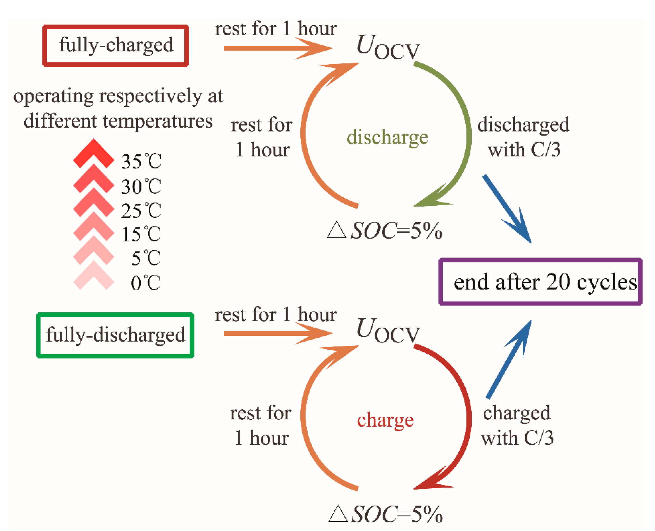
3.2. Characteristics of Open Circuit Voltage

The open circuit voltage has a great influence on the output voltage of the battery model, and for the lithium iron phosphate battery, the change of the open circuit voltage with SOC has strong nonlinear and hysteresis characteristics. The open circuit voltage test scheme, considering the influence of different temperatures and charging–discharging state of the battery, is shown in Figure 6, and the test results are shown in Figure 7. The open circuit voltage in the charging and discharging states are almost the same at different temperatures, except there is a large difference between an SOC of less than 0.1 and an SOC greater than 0.95. When SOC = 1, the open circuit voltage increases with the ambient temperature, while, when SOC = 0, the open circuit voltage increases with a decrease in the ambient temperature. However, in order to ensure the safety and cycle life of the battery in the actual use process, the battery may not be fully charged and discharged. Most of the time, the battery works in the state of 0.1 < SOC < 0.9, so the open circuit voltage of the battery could not consider the influence of temperature. However, the open circuit voltage also has a strong hysteresis characteristic, which shows that the SOC–OCV relationship curve in the charging state does not coincide with that in the discharging state, and when the battery is changing state frequently, the OCV needs SOC increases or decreases by a value (which is about 0.1) to change to the corresponding state [37]. Therefore, in the process of open circuit voltage fitting, we need to consider the influence of battery hysteresis on the equivalent circuit terminal voltage. When a battery works in a purely electric vehicle, it is in the discharging state most of the time. Therefore, in order to simplify the algorithm and consider the open circuit voltage hysteresis characteristic, the open circuit voltage test data were processed as follows:

$$U_{\mathrm{OCV}} = (U_{\mathrm{OCV}\_\mathrm{c}} - U_{\mathrm{OCV}\_\mathrm{d}})\ast 0.25 + U_{\mathrm{OCV}\_\mathrm{d}}$$

(14)

In the formula, $U_{\mathrm{OCV}\_\mathrm{c}}$ is the open circuit voltage under the charging state at 30 °C; $U_{\mathrm{OCV}\_\mathrm{d}}$ is the open circuit voltage under the discharging state at 30 °C.

In this paper, a polynomial was used to fit the open circuit voltage, and when using sixth order polynomials, the root mean squared error (RMSE) was 0.0093. The RMSE was 0.0054 when using the seventh order polynomial, and the RMSE was 0.0049 when using the eighth order polynomials. It can be seen that the fitting error decreases with an increase in the polynomial order. However, if the polynomial order is too high, the nonlinearity will increase and the calculation is complex. Therefore, this paper uses the eighth order polynomial to fit the battery open circuit voltage. The fitting results are shown in

Table 1. Results obtained from fitting of the polynomial in Equation (15).

a1	a2	a3	a4	a5	a6	a7	a8	a9
−218.825	1017.918	−1958.44	2013.781	−1194.95	413.3511	−80.8272	8.4897	2.8423

.

$$\begin{array}{l}{U}_{\mathrm{OCV}}=a_1\cdot SO{C}^8+a_2\cdot SO{C}^7+a_3\cdot SO{C}^6+a_4\cdot SO{C}^5+a_5\cdot SO{C}^4+\\ a_6\cdot SO{C}^3+a_7\cdot SO{C}^2+a_8\cdot SOC+a_9\end{array}$$

(15)

4. Parameter Identification of Fractional Equivalent Circuit Model Based on Particle Swarm Optimization (PSO)

4.1. Identification with PSO Algorithm

Compared with the integral model, the fractional model is related to the historical state. The data has a memory effect, which leads to the slow calculation process. As an evolutionary algorithm, particle swarm optimization (PSO) has been widely investigated and applied in recent years due to its advantages of high calculation speed, fewer call parameters and simple programming. In order to further improve the searching ability and convergence speed of the particle swarm optimization algorithm, and to improve its weakness of easily falling into local optimum, the particle swarm optimization algorithm with dynamic inertia weight was used to identify a fractional equivalent circuit model, which can have more weight in the early stage of calculation to expand the searching range and improve the global searching ability and have less weight in the later stage of calculation to carry out local accurate calculation and improve the convergence speed and accuracy of the results. The specific methods are as follows:

1. Initialization

The particle velocity v_max, v_min and the position limit θ_max, θ_min were defined to avoid ignoring the optimal value and result overflow. The velocity v_l,j and the position θ_l,j of random particles were defined, l is the sequence of particles, where l = 1.2.3…N₁, N₁ is the number of particles. In this paper, N₁ = 200. j is the number of iterations. At the beginning, j = 0, the particle position θ_l,j represents the identification parameter set [R₀, R₁, C₁, α₁].

2. Calculation of fitness function

The fitness function is the most important part of the particle swarm optimization algorithm. The fitness function of each particle under the current iteration is

$$Fit(l,j)={\displaystyle \sum _{k=1}^n\left|U_{\mathrm{r}}\left(k\right)-U_{\mathrm{m}}(k,{\theta }_{l,j})\right|}$$

(16)

where n is the amount of test data, U_r(k) is the measured terminal voltage of the battery at k time and $U_{\mathrm{m}}(k,{\theta }_{l,j})$ is the terminal voltage of the fractional order model at particle position of θ_l,j and its calculation method is as follows:

The transfer function of the differential equation of the fractional capacitor is as follows:

$$\frac{U_1(s)}{I_1(s)}=\frac{1}{C_1{s}^{{\alpha }_1}}$$

(17)

Then the terminal voltage at the polarizing ring is:

$$U_1(s)=(I-C_1{s}^{{\alpha }_1}{U}_1)R_1$$

(18)

$$U_1(s)=\frac{I{R}_1}{1+C_1{R}_1{s}^{{\alpha }_1}}$$

(19)

If the voltage at both ends of the polarizing ring and internal resistance is U, then

$$\frac{U(s)}{I(s)}=\frac{U_{\mathrm{ocv}}\left(\mathrm{s}\right)-U_{\mathrm{t}}\left(\mathrm{s}\right)}{I(s)}=\frac{I{R}_0+\frac{I{R}_1}{1+C_1{R}_1{s}^{{\alpha }_1}}}{I}=\frac{R_0+R_0{R}_{1}C1s^{{\alpha }_1}+R_1}{1+C_1{R}_1{s}^{{\alpha }_1}}$$

(20)

Formula (20) is transformed into a fractional order differential equation and combined with the definition of the G–L type, so we can get:

$$U(k)=\frac{h^{\alpha 1}}{h^{\alpha 1}+C_1{R}_1}\left[\left(R_0+R_1\right)I(k)+\frac{R_0{R}_1{C}_1}{h^{\alpha 1}}{\displaystyle \sum _{i=0}^{N\mathrm{c}}\left[\begin{array}{c}-{\alpha }_1\\ i\end{array}\right]I(k-i)}-\frac{C_1{R}_1}{h^{\alpha 1}}{\displaystyle \sum _{i=1}^{N\mathrm{c}}\left[\begin{array}{c}-{\alpha }_1\\ i\end{array}\right]U(k-i)}\right]$$

(21)

Then

$$U_{\mathrm{m}}(k,{\theta }_{l,j})=U_{\mathrm{OCV}}(SOC(k\left)\right)-U(k)$$

(22)

where h is the sampling interval, which is 0.2 s in this paper; N_c is the quantity of historical data participating in the calculation, which should be the number of all data points before k time in theory, but the quantity of calculations will increase sharply with the iteration time [30]. Therefore, this paper comprehensively considered the calculation quantity of particle swarm optimization and the precision of output voltage of the fractional order model, and set the calculation truncation quantity N_e = 800, when k > N_e, N_c = N_e, k ≤ N_e, N_c = k.

3. Update of individual optimal fitness

The fitness value Fit(l,j) corresponding to the position θ_l,j under the current iteration time of each particle is compared with the fitness value F_best(l) corresponding to the historical best position of the particle ${\theta }_l^{\mathrm{best}}$. If Fit(l,j) < F_best(l), the historical best position of the particle is updated with the current particle position ${\theta }_l^{\mathrm{best}}$.

4. Update of the best group fitness

The fitness value Fit(l,j) corresponding to the position θ_l,j under the current iteration time of each particle is compared with the fitness value F_best corresponding to the global optimal position ${\theta }^{\mathrm{best}}$. If Fit(l,j) < F_best, the global optimal position is updated with the current particle position ${\theta }^{\mathrm{best}}$.

5. Update particle position and speed

Update the speed of each particle:

$$v_{l,j+1}=({\omega }_2-\frac{({\omega }_2-{\omega }_1)j}{M})v_{l,j}+c_1{r}_1({\theta }_l^{\mathrm{best}}-{\theta }_{l,j})+c_2{r}_2({\theta }^{\mathrm{best}}-{\theta }_{l,j})$$

(23)

where ω₁, ω₂ are weights to adjust the search range. In this paper, ω₁ = 0.4, ω₂ = 0.9; M is the maximum number of iterations, M = 200; c₁, c₂ are acceleration constants, c₁ = c₂ = 2; r₁, r₂ are random parameters, taking the range [0,1] to increase the randomness of the particle.

Update particle position:

$${\theta }_{l,j+1}={\theta }_{l,j}+v_{l,j+1}$$

(24)

6. Judge whether the program is over

If the number of large iterations or the fitness value is less than the default value, then the algorithm ends, and the global optimal position ${\theta }^{\mathrm{best}}$ is the optimal solution, otherwise, to the number of iterations add 1 and return to step 2.

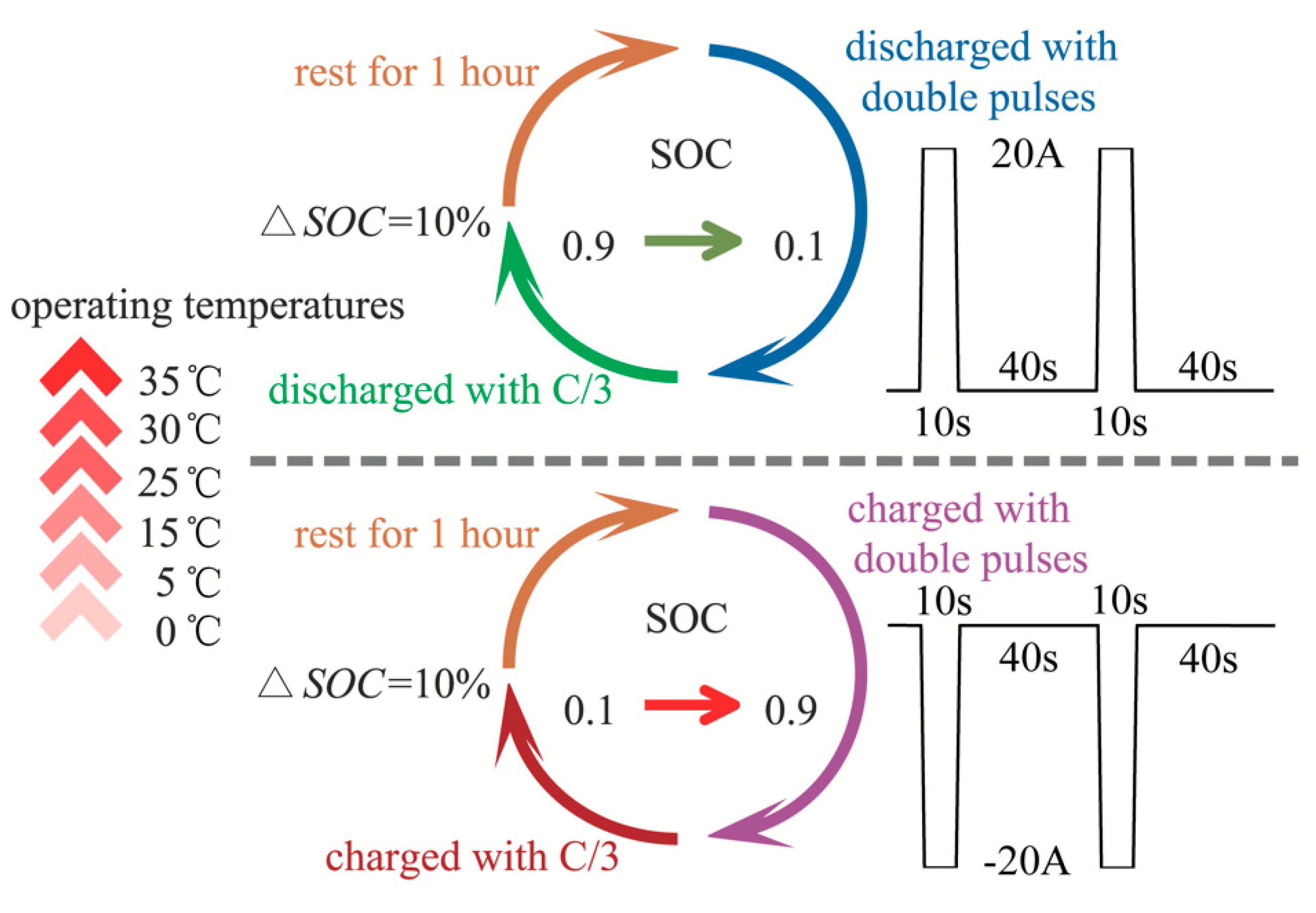
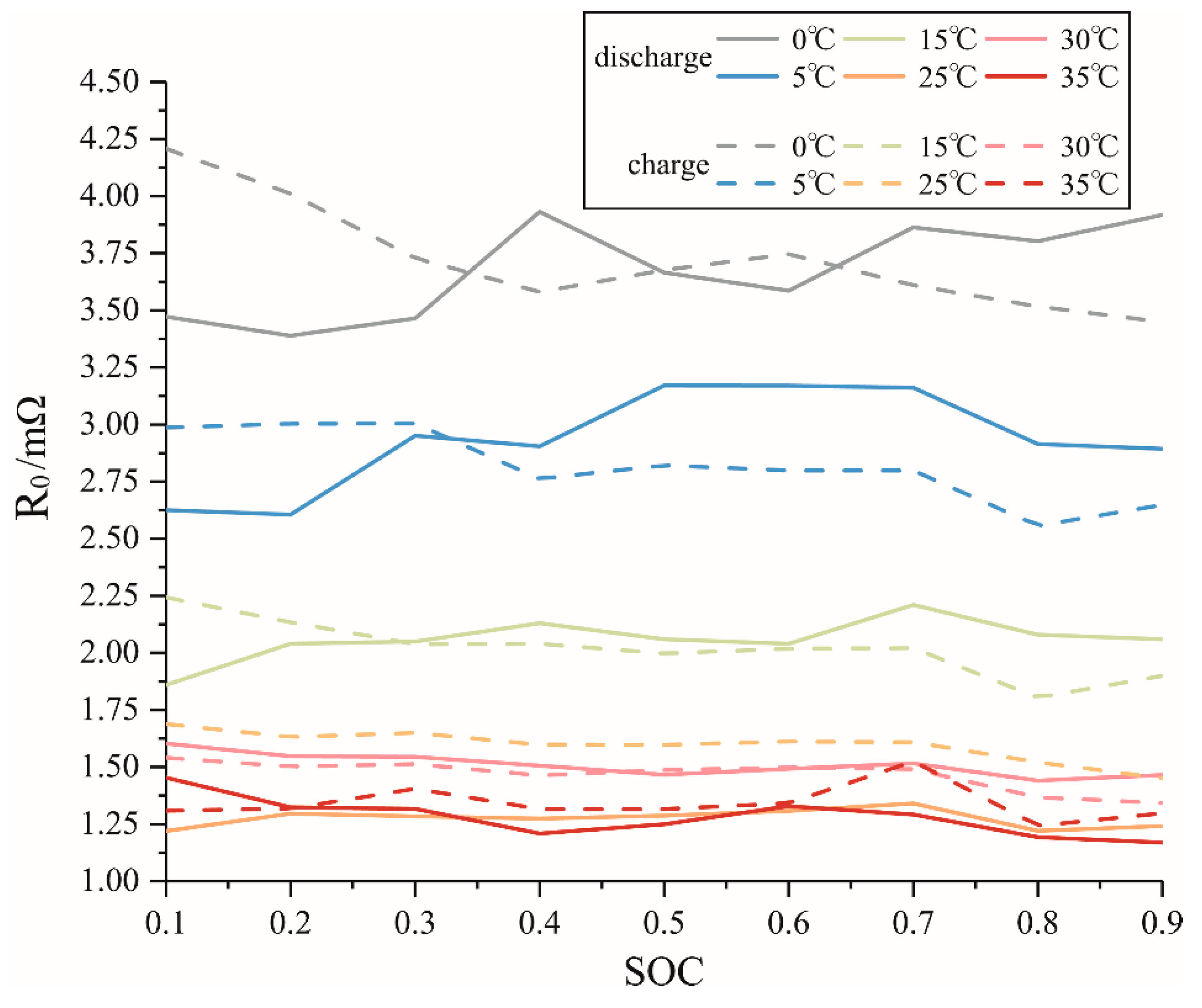
4.2. Identification Test and Results

The change of battery state is complex when the battery is in the working process, and its equivalent circuit model parameters will change with its own factors and external state. In order to obtain accurate parameters of the fractional equivalent circuit model, a double pulse test was carried out under different charging and discharging states, SOC and ambient temperatures to excite the battery characteristics. The pulse current is ±20 A, the duration is 10 s and the rest time is 40 s. The test scheme is shown in Figure 8.

Taking the ambient temperature of 30 °C as an example, the terminal voltage of the fractional equivalent circuit model is compared with the integer equivalent circuit model under identification conditions, and the results are shown in Figure 9 and Figure 10.

As can be seen from the figure above, the terminal voltage of the fractional model is in good agreement with the measured voltage when current is loading or unloading, and it can better fit the resistance and capacitance characteristics of the battery at the charging–discharging state and static state. Although the integer model can roughly fit the measured voltage, it has a big error with the measured voltage at the moment of current loading and unloading due to the model order and characteristics of the integer model. The fitting error of the fractional order model is smaller than that of the integral order model in the same model order, and it can better simulate the battery characteristics of resistance and capacitance.

The identification results of fractional equivalent circuit model parameters in charging–discharging states, different ambient temperatures and SOC are shown in Figure 11, Figure 12, Figure 13 and Figure 14.

The internal resistance R₀ at different ambient temperatures fluctuates in a certain range, but the change of SOC in a low-temperature environment is more drastic than that in a high-temperature environment. The difference of internal resistance in charging and discharging states is small, and the resistance value increases with a decrease in temperature in most cases. The polarization internal resistance R₁ fluctuates more drastically at low temperatures than R₀, but it has less impact at high temperatures in most cases. The value of R₁ decreases with an increase in the ambient temperature. The fluctuation degree of the polarization capacitance C₁ in the fractional model has little correlation with the ambient temperature, and its value increases with the ambient temperature in charging and discharging states, and the capacitance value varies greatly in different ambient temperatures; the trend of the fractional order α₁ is consistent with polarization capacitance C₁, and increases with the temperature in most cases. According to the four parameter identification results, the internal resistance, polarization resistance, capacitance and order of CPE elements in the first order fractional equivalent circuit model are the temperature-sensitive elements, as they all change with the ambient temperature, but the sensitivity is different.

In the following calculation process, the parameters identified in this paper were used as key points to fit the parameters under other conditions using the two-dimensional quadratic spline interpolation method, so as to meet all environmental temperatures and SOC conditions.

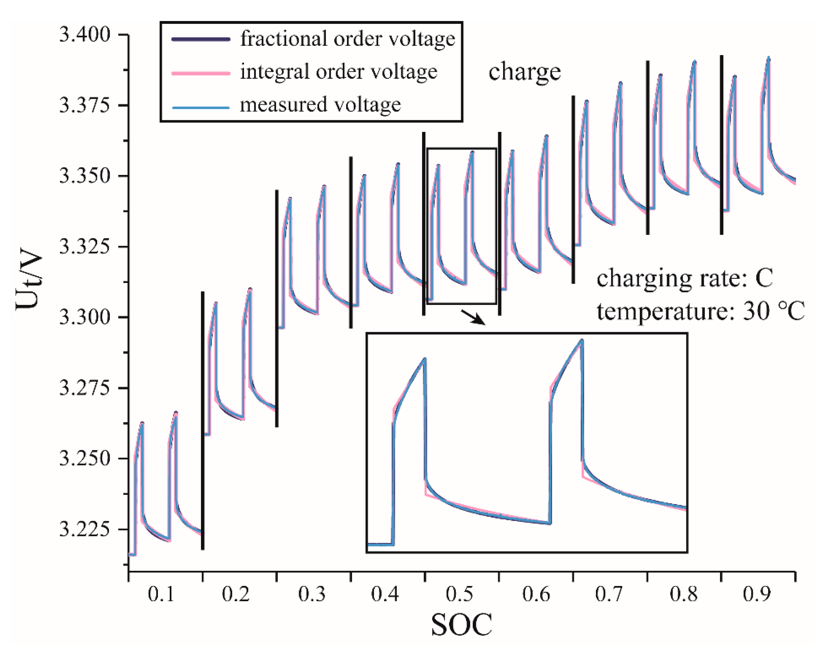
4.3. Verification of Identification Results

The dynamic stress test (DST) is simplified from the Federal Urban Driving Schedule (FUDS), which consists of 10 discharging stages, five charging stages and five static stages. The duration of each cycle is 360 s. The DST can simulate the actual operation condition of the battery well, so it is a common simulated condition to verify the accuracy of battery equivalent circuit models and the validity of SOC estimation methods. In this paper, 26 continuous DST cycles were used to test the battery. The ambient temperature is 28 °C. The conditions of one DST are shown in

Table 2. Current and duration of dynamic stress test (DST).

Order	Current I/A	Duration/s	Order	Current I/A	Duration/s
1	0	16	11	10	12
2	5	28	12	−5	8
3	10	12	13	0	16
4	−5	8	14	5	36
5	0	16	15	40	8
6	5	24	16	25	24
7	10	12	17	−10	8
8	−5	8	18	10	32
9	0	16	19	−17	8
10	5	24	20	0	44

. The comparisons of terminal voltage with the fractional order model, terminal voltage with the integer order model and measured voltage are shown in Figure 15. The error between measured voltage and model terminal voltage is shown in Figure 16.

The terminal voltage of the fractional order model can track the measured voltage well. The average error of voltage in the fractional order model is 0.0034 V and the relative error is 0.107%. The error is large only when the current is large. The maximum error is 0.0196 V and the maximum relative error is 0.613%. The terminal voltage of the integral order model is larger than the measured voltage and terminal voltage of the fractional model. The average error of voltage in the integral order model is 0.0086 V, and the relative error is 0.269%. Therefore, the parameter of the fractional order model based on PSO and the SOC-OCV simplified model considering the hysteresis characteristics can simulate the characteristics of battery voltage well, which can provide higher precision of model terminal voltage to estimate battery SOC using a fractional Kalman filter.

5. Estimation for SOC Based on Fractional Extended Kalman Filter (FEKF)

A Kalman filter is an optimal estimation method based on minimum variance estimation [38], but it is only applicable to linear systems. However, the vehicle power battery has strong nonlinear characteristics in the actual operation process. As an improved form of the Kalman filter, the extended Kalman filter can solve this problem well, and has a wide application in SOC estimation.

5.1. Iterative Formula of FEKF

The linearization method of the extended Kalman filterbased on the fractional order model is the same as the integer order extended Kalman filter, and the nonlinear part is replaced by a Jacobian matrix:

Combined with Formulas (11) and (12), the one-step prediction of state is:

$$\widehat{x}(k+1|k)=A\widehat{x}(k|k)+BI(k)-O$$

(25)

$$\widehat{x}(k+1|k)={\left[SOC(k+1|k),U_1(k+1|k)\right]}^{\mathrm{T}}$$

(26)

$$\mathbf{O}=\left[\begin{array}{c}0\\ {\displaystyle \sum _{i=1}^{N\mathrm{c}}\left[\begin{array}{c}-{\alpha }_1\\ i\end{array}\right]}{U}_1(k+1-i)\end{array}\right]$$

(27)

The one-step prediction of covariance is:

$$\begin{array}{l}\mathbf{P}(k+1|k)=\mathrm{E}\left[\right(x(k+1)-\widehat{x}(k+1|k\left)\right)(x(k+1)-\widehat{x}(k+1|k{\left)\right)}^{\mathrm{T}}]\\ =(A-\mathrm{diag}\{0,\left[\begin{array}{c}-{\alpha }_1\\ i\end{array}\right]\})P(k){(A-\mathrm{diag}\{0,\left[\begin{array}{c}-{\alpha }_1\\ i\end{array}\right]\})}^{\mathrm{T}}+{\displaystyle \sum _{i=2}^{N\mathrm{c}}\mathrm{diag}\{0,\left[\begin{array}{c}-{\alpha }_1\\ i\end{array}\right]\}}P(k+1-i)\mathrm{diag}\{0,\left[\begin{array}{c}-{\alpha }_1\\ i\end{array}\right]{\}}^{\mathrm{T}}+Q\end{array}$$

(28)

The gain matrix of the Kalman filter is:

$$K(k+1)=P(k+1|k)H^{\mathrm{T}}{(HP(k+1|k)H^{\mathrm{T}}+R)}^{-1}$$

(29)

H is a Jacobian matrix to replace the nonlinear function h in Equation (12):

$$H=\left[\begin{array}{ccc}\frac{\partial U_{\mathrm{OCV}}\left(SOC\right)}{SOC(k+1|k)}& -1& -1\end{array}\right]$$

(30)

The error of observation is:

$$\epsilon (k+1)=Y(k+1)-\widehat{y}(k+1)$$

(31)

$$\widehat{y}(k+1)=U_{\mathrm{OCV}}\left(SOC\right(k+1|k\left)\right)-U_1(k+1|k)-R_0\ast I(k+1)$$

(32)

Y(k + 1) is the measured voltage at k + 1.

Covariance matrix update:

$$P(k+1)=(I_{2\mathrm{x}2}-K(k+1)H)P(k+1|k)$$

(33)

$I_{2\mathrm{x}2}$ is a two-dimensional identity matrix.

State update:

$$\widehat{x}(k+1|k+1)=\widehat{x}(k+1|k)+K(k+1)\epsilon (k+1)$$

(34)

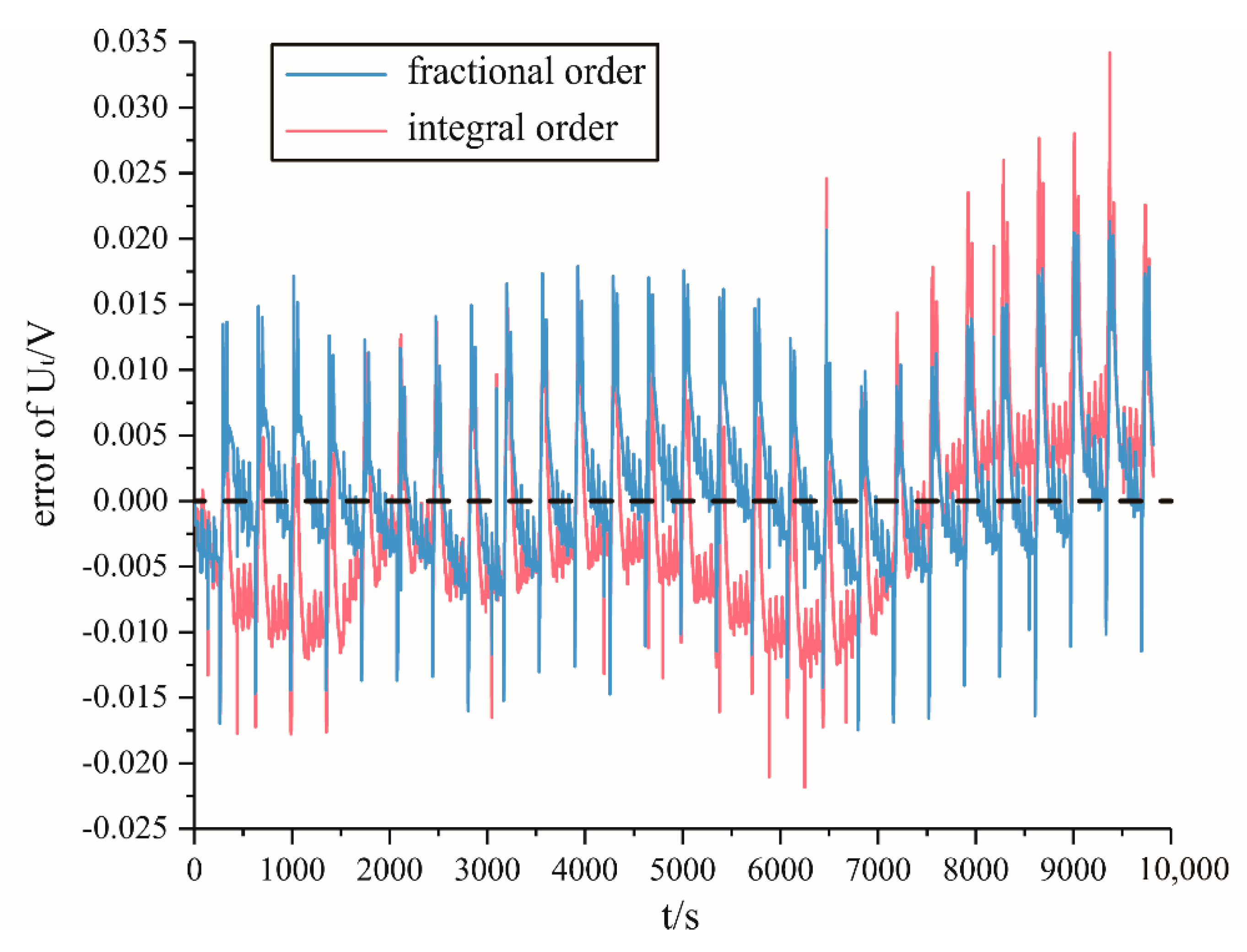
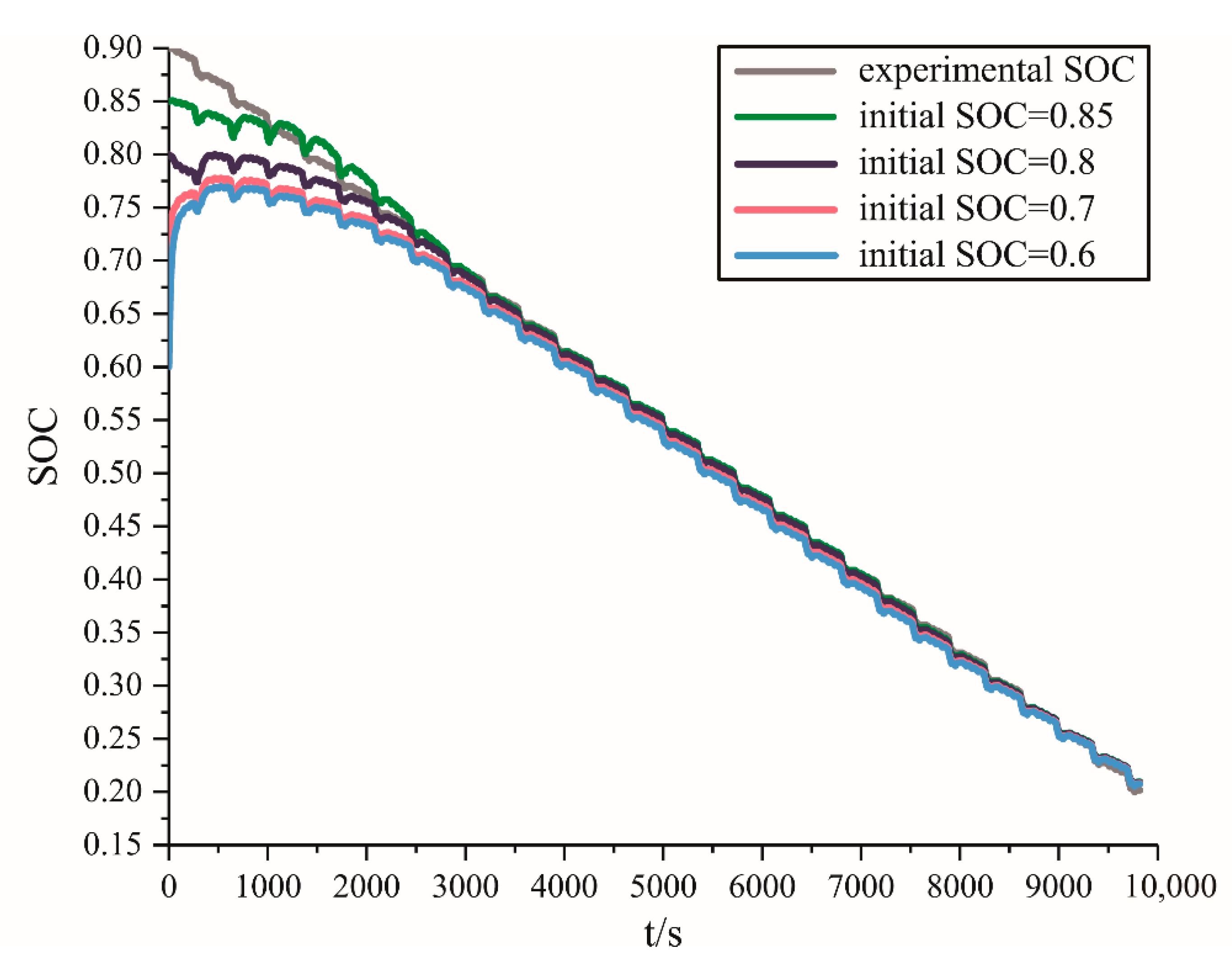
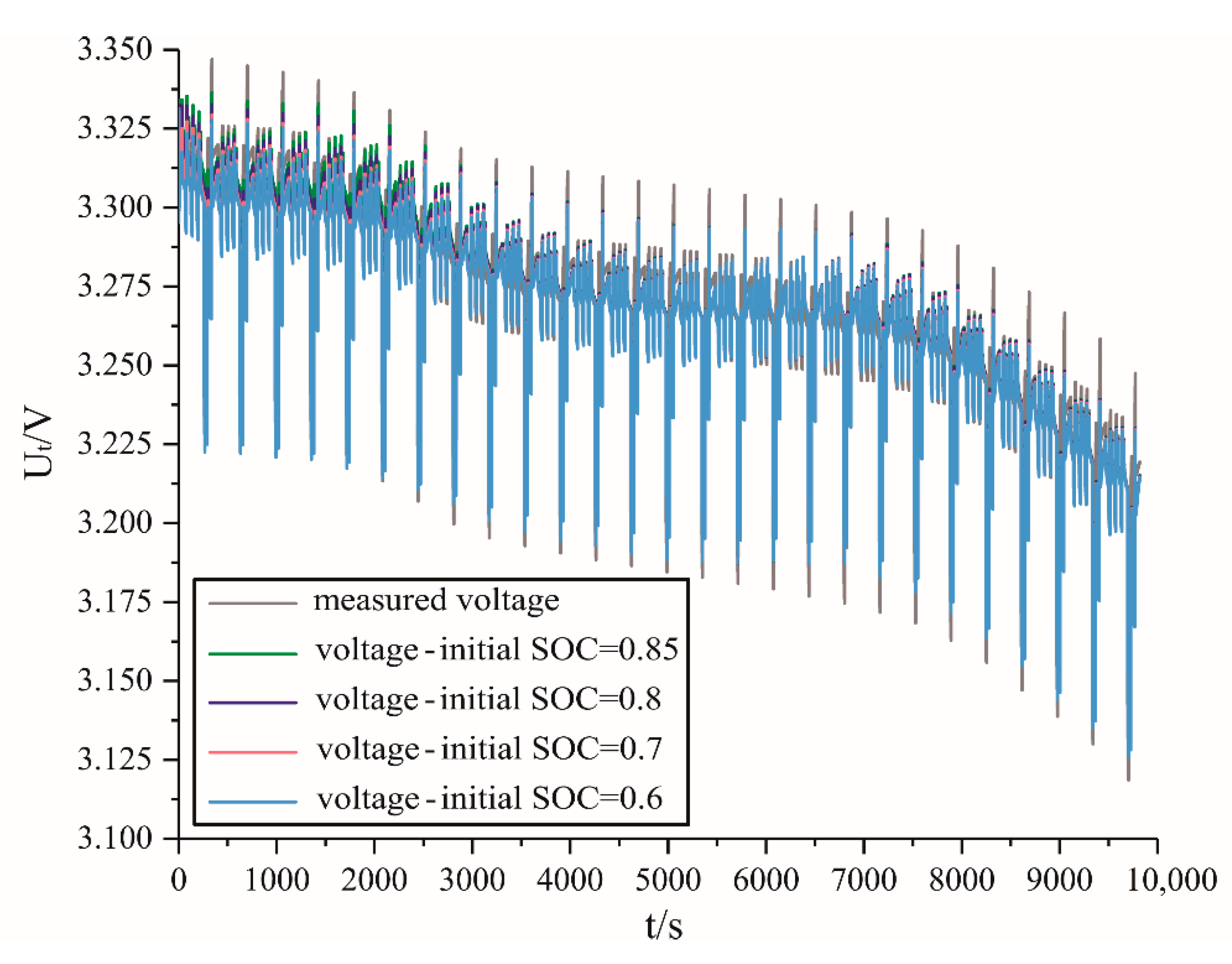
5.2. Verification of Estimation Results

The environmental temperature is set at 28 °C and the working condition is 26 continuous DST conditions. The FEKF was verified and compared with the integer order EKF. The initial SOC of the FEKF and EKF was the same as the initial value of the operating condition. The comparison results of SOC estimation in two filters are shown in Figure 17, and the errors between test value and SOC estimation are shown in Figure 18. The comparison between the measured voltage and the output voltage of the two filters is shown in Figure 19, and the error of terminal voltage is shown in Figure 20.

The error of the FEKF and EKF is relatively large in the early stage of estimation, but after a period of time, the FEKF can quickly keep up with the true SOC value and make the error fluctuate around 0. The average error and relative error of SOC estimated by the FEKF and EKF is shown in

Table 3. Error comparison between FEKF and EKF.

Method	Average Error	Relative Error
FEKF	0.0036	0.52%
EKF	0.0224	3.2%

. Because the accuracy of the fractional order model is higher than that of the integer order model, the output voltage of the FEKF can follow the measured voltage better than the EKF. Moreover, due to the effect of covariance, compared with the output voltage error of the equivalent circuit model without a filter effect in Section 4.3, the terminal voltage error can fluctuate around 0, thus achieving a good balance between model reliability and measurement reliability.

In this paper, when the noise covariance and initial covariance are the same as above, the initial SOC is set as 0.85, 0.8, 0.7 and 0.6 to verify the robustness of the FEKF. The estimation results and errors of SOC are shown in Figure 21 and Figure 22, and the output voltage and error are shown in Figure 23 and Figure 24.

In the case of different initial errors, the SOC and the output voltage estimated by the FEKF can achieve a good convergence effect after a period of time. When the initial error is large, the FEKF can make the error decrease rapidly in the early stage and ensure a good convergence speed. At the beginning of the simulation, the error of output voltage increases with the initial SOC error, and this is due to the existence of an initial SOC error, which leads to a decrease in model open circuit voltage and terminal voltage. However, with the feedback of the measured voltage, the estimated state will gradually converge to the test value.

In conclusion, the proposed FEKF can estimate the battery SOC more accurately than the EKF and has strong robustness.

6. Conclusions

In this paper, the equivalent circuit model based on fractional order theory was established. The characteristics of battery capacity and open circuit voltage at different temperatures were studied. A simplified modeling method considering hysteresis characteristics of open circuit voltage was proposed. Based on the PSO method, the parameters of the fractional order model were identified at different temperatures. Finally, the fractional extended Kalman filter was established. The advantages of the proposed estimation method are as follows:

1. In the same order, compared with the integer order equivalent circuit model, the fractional order model can accurately simulate the characteristics of resistance and capacitance when the battery is charging, discharging or static;

2. It can ensure the accuracy of the output voltage of the fractional order model when the battery is in a wide range of temperatures and the battery state changes frequently. Compared with measured voltage in continuous DST conditions, the average error of voltage in the integral order model is 0.0086 V, and the relative error is 0.269%, but the average error of voltage in the fractional order model is 0.0034 V and the relative error is 0.107%, which can provide a more accurate model of output voltage for fractional estimators;

3. In the same conditions of initial SOC and temperature, compared with the integer extended Kalman filter, the fractional extended Kalman filter can estimate battery SOC more accurately in continuous DSTs, and the average error of SOC estimated by the FEKF is 0.0036 and the relative error is 0.52% when average error and relative error by the EKF are 0.0224 and 3.2%. The FEKF also has strong robustness when the initial error is large, and it can make the error of SOC decrease rapidly in the early stage and ensure a good convergence speed.

References

1. Wang, A.C.; Zhang, Y.; Zuo, H.F. Assessing the Performance Degradation of Lithium-Ion Batteries Using an Approach Based on Fusion of Multiple Feature Parameters. Math. Probl. Eng. 2019, 7, 1–12. [Google Scholar] [CrossRef]
2. Tian, J.; Wang, Q.; Ding, J.; Wang, Y.Q.; Ma, Z.S. Integrated Control with, D.Y.C and, D.S.S for 4WID Electric Vehicles. IEEE Access 2019, 7, 124077–124086. [Google Scholar] [CrossRef]
3. Cheng, K.W.E.; Divakar, B.P.; Wu, H.J.; Ding, K.; Ho, H.F. Battery-Management System (BMS) and, S.O.C Development for Electrical Vehicles. IEEE Trans. Veh. Technol. 2011, 60, 76–88. [Google Scholar] [CrossRef]
4. Guo, J.G.; Dong, H.X.; Sheng, W.H.; Tu, C. Optimum control strategy of regenerative braking energy for electric vehicle. J. Jiangsu Univ. (Nat. Sci. Ed.) 2018, 39, 132–138. [Google Scholar] [CrossRef]
5. Dai, H.F.; Wei, X.Z.; Sun, Z.C.; Wang, J.Y.; Gu, W.J. Online cell, S.O.C estimation of Li-ion battery packs using a dual time-scale Kalman filtering for, E.V. applications. Appl. Energy 2012, 95, 227–237. [Google Scholar] [CrossRef]
6. Wang, S.Q.; Verbrugge, M.; Wang, J.S.; Liu, P. Multi-parameter battery state estimator based on adaptive and direct solution of the governing differential equations. J. Power Sources 2011, 196, 8735–8741. [Google Scholar] [CrossRef]
7. Hu, Y.; Yurkovich, S. Battery cell state-of-charge estimation using linear parameter varying system techniques. J. Power Sources 2012, 198, 338–350. [Google Scholar] [CrossRef]
8. Tian, Y.; Xia, B.Z.; Sun, W.; Xu, Z.H.; Zheng, W.W. A modified model based state of charge estimation of power lithium-ion batteries using unscented Kalman filter. J. Power Sources 2014, 270, 619–626. [Google Scholar] [CrossRef]
9. Chemali, E.; Kollmeyer, P.J.; Preindl, M.; Ahmed, R.; Emadi, A. Long Short-Term Memory Networks for Accurate State-of-Charge Estimation of Li-ion Batteries. IEEE Trans. Ind. Electron. 2018, 65, 6730–6739. [Google Scholar] [CrossRef]
10. Chemali, E.; Kollmeyer, P.J.; Preindl, M.; Ahmed, R.; Emadi, A. State-of-charge estimation of Li-ion batteries using deep neural networks: A machine learning approach. J. Power Sources 2018, 400, 242–255. [Google Scholar] [CrossRef]
11. Xia, B.Z.; Cui, D.Y.; Sun, Z.; Lao, Z.Z.; Zhang, R.F.; Wang, W.; Sun, W.; Lai, Y. State of charge estimation of lithium-ion batteries using optimized Levenberg-Marquardt wavelet neural network. Energy 2018, 153, 694–705. [Google Scholar] [CrossRef]
12. Tian, Y.; Li, D.; Tian, J.D.; Xia, B.Z. State of charge estimation of lithium-ion batteries using an optimal adaptive gain nonlinear observer. Electrochim. Acta 2017, 225, 225–234. [Google Scholar] [CrossRef]
13. Rivera-Barrera, J.P.; Muñoz-Galeano, N.; Sarmiento-Maldonado, H.O. SoC Estimation for Lithium-ion Batteries: Review and Future Challenges. Electronics 2017, 6, 102. [Google Scholar] [CrossRef] [Green Version]
14. Awadallah, M.A.; Venkatesh, B. Accuracy improvement of, S.O.C estimation in lithium-ion batteries. J. Energy Store 2016, 6, 95–104. [Google Scholar] [CrossRef]
15. Huang, K.; Guo, Y.F.; Li, Z.G. Review of state of charge estimation methods for power lithium-ion battery. Chin. J. Power Sources 2018, 42, 1395–1401. Available online: http://kns.cnki.net/KCMS/detail/detail.aspx?FileName=DYJS201809051&DbName=CJFQ2018 (accessed on 11 November 2020).
16. Jiang, C.Y.; Wang, W.C.; Yang, X.P. Modeling and, S.O.C calculations of hybrid electrical vehicles (HEV) powered by lithium iron phosphate batteries. Energy Storage Sci. Technol. 2018, 7, 897–901. [Google Scholar] [CrossRef]
17. Tong, S.J.; Lacap, J.H.; Park, J.W. Battery state of charge estimation using a load-classifying neural network. J. Energy Storage 2016, 7, 236–243. [Google Scholar] [CrossRef]
18. Sheikhan, M.; Pardis, R.; Gharavian, D. State of charge neural computational models for high energy density batteries in electric vehicles. Neural Comput. Appl. 2013, 22, 1171–1180. [Google Scholar] [CrossRef]
19. Álvarez Antón, J.C.; García Nieto, P.J.; de Cos Juez, F.J.; Sánchez Lasheras, F.; González Vega, M.; Roqueñí Gutiérrez, M.N. Battery state-of-charge estimator using the, S.V.M technique. Appl. Math. Model. 2013, 37, 6244–6253. [Google Scholar] [CrossRef]
20. Charkhgard, M.; Farrokhi, M. State-of-Charge Estimation for Lithium-Ion Batteries Using Neural Networks and, E.K.F. IEEE Trans. Ind. Electron. 2010, 57, 4178–4187. [Google Scholar] [CrossRef]
21. He, W.; Williard, N.; Chen, C.C.; Pecht, M. State of charge estimation for Li-ion batteries using neural network modeling and unscented Kalman filter-based error cancellation. Int. J. Electr. Power Energy Syst. 2014, 62, 783–791. [Google Scholar] [CrossRef]
22. Du, S.Y.; Tang, Z.; Chen, D. Research on, S.O.C estimation methods for lead-acid batteries based on fuzzy control. Power Electron. 2017, 51, 95–97. Available online: http://kns.cnki.net/KCMS/detail/detail.aspx?FileName=DLDZ201712030&DbName=CJFQ2017 (accessed on 11 November 2020).
23. Sheng, H.M.; Xiao, J. Electric vehicle state of charge estimation: Nonlinear correlation and fuzzy support vector machine. J. Power Sources 2015, 281, 131–137. [Google Scholar] [CrossRef]
24. Dong, G.Z.; Chen, Z.H.; Wei, J.W.; Zhang, C.B.; Wang, P. An online model-based method for state of energy estimation of lithium-ion batteries using dual filters. J. Power Sources 2016, 301, 277–286. [Google Scholar] [CrossRef]
25. Liu, C.Z.; Liu, W.Q.; Wang, L.Y.; Hu, G.D.; Ma, L.P.; Ren, B.Y. A new method of modeling and state of charge estimation of the battery. J. Power Sources 2016, 320, 1–12. [Google Scholar] [CrossRef]
26. Lu, X.; Li, H.; Xu, J.; Chen, S.Y.; Chen, N. Rapid Estimation Method for State of Charge of Lithium-Ion Battery Based on Fractional Continual Variable Order Model. Energies 2018, 11, 714. [Google Scholar] [CrossRef] [Green Version]
27. Wang, B.J.; Li, S.B.E.; Peng, H.; Liu, Z.Y. Fractional-order modeling and parameter identification for lithium-ion batteries. J. Power Sources 2015, 293, 151–161. [Google Scholar] [CrossRef]
28. He, Y.; Qin, S.X.; Liu, X.T.; Zheng, X.X.; Zeng, G.J. Power Battery, S.O.C Estimation Based on Fractional Unscented Particle Filter. Automob. Technol. 2018, 5, 6–11. [Google Scholar] [CrossRef]
29. Wang, Y.J.; Zhang, C.B.; Chen, Z.H. An adaptive remaining energy prediction approach for lithium-ion batteries in electric vehicles. J. Power Sources 2016, 305, 80–88. [Google Scholar] [CrossRef]
30. Sun, F.C.; Xiong, R.; He, H.W. Estimation of state-of-charge and state-of-power capability of lithium-ion battery considering varying health conditions. J. Power Sources 2014, 259, 166–176. [Google Scholar] [CrossRef]
31. Xiong, R.; Zhang, X.W.; Sun, F.C.; Fan, J.X. State-of-Charge Estimation of the Lithium-Ion Battery Using an Adaptive Extended Kalman Filter Based on an Improved Thevenin Model. IEEE Trans. Veh. Technol. 2011, 60, 1461–1469. [Google Scholar] [CrossRef]
32. Cheng, Z.; Lv, J.K.; Liu, J.G.; Wang, L. Application of equivalent hysteresis model in estimation of state of charge of lithium-ion battery. J. Hunan Univ. (Nat. Sci.) 2015, 42, 63–70. [Google Scholar] [CrossRef]
33. Ou, Y.J. The Research for Lithium Ion Power Battery, S.O.C Estimation and, S.O.F Evaluation of Electric Vehicles. Ph.D. Thesis, South China University of Technology, Guangzhou, China, 2016. Available online: http://kns.cnki.net/KCMS/detail/detail.aspx?FileName=1016737137.nh&DbName=CDFD2017 (accessed on 11 November 2020).
34. Lee, S.; Kim, J.; Lee, J.; Cho, B.H. State-of-charge and capacity estimation of lithium-ion battery using a new open-circuit voltage versus state-of-charge. J. Power Sources 2008, 185, 1367–1373. [Google Scholar] [CrossRef]
35. Wei, J.W.; Dong, G.Z.; Chen, Z.H. On-board adaptive model for state of charge estimation of lithium-ion batteries based on Kalman filter with proportional integral-based error adjustment. J. Power Sources 2017, 365, 308–319. [Google Scholar] [CrossRef]
36. Wang, B.J. Modeling and State Estimation for Lithium-Ion Batteries Based on Fractional Calculus. Ph.D. Thesis, Harbin Institute of Technology, Harbin, China, 2016. [Google Scholar]
37. Weng, C.H.; Sun, J.; Peng, H. A unified open-circuit-voltage model of lithium-ion batteries for state-of-charge estimation and state-of-health monitoring. J. Power Sources 2014, 258, 228–237. [Google Scholar] [CrossRef]
38. Kalman, R.E. On the general theory of control systems. Ifac Proc. Vol. 1960, 1, 491–502. [Google Scholar] [CrossRef]
Figure 1. Structure of the article.
Energies 13 05947 g001
Figure 2. Fractional equivalent circuit model with a constant phase element (CPE).
Energies 13 05947 g002
Figure 3. Scheme of discharging–charging capacity test at different temperatures in the range 0–35 °C and rates.
Energies 13 05947 g003
Figure 4. Evolution of the discharging capacity as a function of rate at different temperatures in the range 0–35 °C.
Energies 13 05947 g004
Figure 5. Evolution of the charging capacity as a function of rate at different temperatures in the range 0–35 °C.
Energies 13 05947 g005
Figure 6. Scheme of discharging–charging open circuit voltage test at different temperatures in the range 0–35 °C.
Energies 13 05947 g006
Figure 7. Open-circuit voltage as a function of the state of charge (SOC) at different temperatures in the range 0–35 °C for the A123 battery.
Energies 13 05947 g007
Figure 8. Scheme of parameter identification test using double pulses under charging–discharging states at different temperatures in the range 0–35 °C.
Energies 13 05947 g008
Figure 9. Terminal voltage fitting results from discharging identification test at 30 ℃ in different SOC.
Energies 13 05947 g009
Figure 10. Terminal voltage fitting results from charging identification test at 30 ℃ in different SOC.
Energies 13 05947 g010
Figure 11. Evolution of the internal resistance R0 as a function of SOC at different temperatures in the range 0–35 °C.
Energies 13 05947 g011
Figure 12. Evolution of the polarization resistance R1 as a function of SOC at different temperatures in the range 0–35 °C.
Energies 13 05947 g012
Figure 13. Evolution of the CPE capacitance C1 as a function of SOC at different temperatures in the range 0–35 °C.
Energies 13 05947 g013
Figure 14. Evolution of the CPE order α1 as a function of SOC at different temperatures in the range 0–35 °C.
Energies 13 05947 g014
Figure 15. Comparison of terminal voltage between fractional model and integral model under 26 continuous DST conditions at 28 °C.
Energies 13 05947 g015
Figure 16. Comparison of terminal voltage errors between fractional model and integral model under 26 continuous DST conditions at 28 °C.
Energies 13 05947 g016
Figure 17. Comparison of SOC filtered by FEKF and EKF under 26 continuous DST conditions at 28 °C.
Energies 13 05947 g017
Figure 18. Comparison of SOC errors between FEKF and EKF under 26 continuous DST conditions at 28 °C.
Energies 13 05947 g018
Figure 19. Comparison of battery terminal voltage filtered by FEKF and EKF under 26 continuous DST conditions at 28 °C.
Energies 13 05947 g019
Figure 20. Comparison of terminal voltage errors between FEKF and EKF under 26 continuous DST conditions at 28 °C.
Energies 13 05947 g020
Figure 21. Comparison of SOC filtered by FEKF in different SOC initial errors under 26 continuous DST conditions at 28 °C.
Energies 13 05947 g021
Figure 22. Comparison of SOC errors filtered by FEKF in different SOC initial errors under 26 continuous DST conditions at 28 °C.
Energies 13 05947 g022
Figure 23. Comparison of terminal voltage filtered by FEKF in different SOC initial errors under 26 continuous DST conditions at 28 °C.
Energies 13 05947 g023
Figure 24. Comparison of terminal voltage errors filtered by FEKF in different SOC initial errors under 26 continuous DST conditions at 28 °C.
Energies 13 05947 g024