An Analytical Model for Production Analysis of Hydraulically Fractured Shale Gas Reservoirs Considering Irregular Stimulated Regions

Abstract

Shale gas reservoirs are typically developed by multistage, propped hydraulic fractures. The induced fractures have a complex geometry and can be represented by a high permeability region near each fracture, also called stimulated region. In this paper, a new integrative analytical solution coupled with gas adsorption, non-Darcy flow effect is derived for shale gas reservoirs. The modified pseudo-pressure and pseudo-time are defined to linearize the nonlinear partial differential equations (PDEs) and thus the governing PDEs are transformed into ordinary differential equations (ODEs) by integration, instead of the Laplace transform. The rate vs. pseudo-time solution in real-time space can be obtained, instead of using the numerical inversion for Laplace transform. The analytical model is validated by comparison with the numerical model. According to the fitting results, the calculation accuracy of analytic solution is almost 99%. Besides the computational convenience, another advantage of the model is that it has been validated to be feasible to estimate the pore volume of hydraulic region, stimulated region, and matrix region, and even the shape of regions is irregular and asymmetrical for multifractured horizontal wells. The relative error between calculated volume and given volume is less than 10%, which meets the engineering requirements. The model is finally applied to field production data for history matching and forecasting.

1. Introduction

Unconventional hydrocarbon resources such as tight and shale oil/gas store in tight formations with ultra-low permeability. With the development of hydraulic fracturing technologies, multifractured horizontal wells (MFHWs) have rapidly emerged as the primary means for exploiting this type of resource. Meanwhile, some technologies are utilized, such as foam injection and carbon dioxide injection [1,2] on recovery enhancement, and photo-Fenton and floatation on sustainable management of flow-back water after hydraulic fracturing [3]. In unconventional reservoirs, due to the propagation of fractures in different directions, branch fractures will be created around the main hydraulic fractures, which have a significant impact on the pressure and rate transient analysis for the fluid flow in the reservoirs.

In order to analyze production data and make long-term forecasts, analytical and numerical tools have been developed. Among them, a large number of numerical approaches [4,5,6,7,8], such as finite element method and boundary element method, are adopted to study the multiple flow mechanisms and fracture characteristics in shale gas reservoirs. Compared with the numerical models, the analytical models are simpler to set up and require fewer original data. Therefore, they are widely used in practice for field applications. Extensive studies have focused on analyzing production data of transient flow period for such complex systems [9,10,11,12,13,14]. Lee et al. [15] derived a tri-linear model to represent the transient flow behavior within a single fracture in an infinite homogeneous reservoir. Wattenbarger et al. [16] proposed an analytical solution accounting for transient linear flow contributions from each region for a fracture with infinite conductivity in a closed reservoir. El-Banbi [17] and Bello et al. [18] extended previous analytical models to develop a series of linear dual-porosity solutions for fluid flow in tight reservoirs, where constant-rate and constant-pressure inner boundaries were considered. Ozkan et al. [19] and Brown et al. [20] extended the concept of tri-linear flow and presented a solution to simulate the pressure-transient behavior in three flow regions, including the hydraulic fracture, the inner region between hydraulic fractures, and the outer region beyond the tip of hydraulic fractures. Stalgorova et al. [21] and Heidari et al. [22] introduced an enhanced-fracture-region (EFR) model to consider the cases where branch fractures cover the interfracture region. Mahdi et al. [23] firstly provided the transient shape factor among different regions in the triple-porosity model.

The models represent an excellent attempt to capture reservoir parameters and flow characteristics for the complex system associated with the MFHWs. However, most analytical solutions were derived by Laplace transformation [17,18,19,20,21,22,23] and Boltzmann’s transformation [24]. Numerical inversion algorithm [25] is needed to transform the Laplace space into real-time space. In order to avoid the inconvenience of Laplace transformation, several approximated analytical solutions have been presented. Shahamat et al. [26] introduced the concept of continuous succession of pseudo-steady states based on the capacitance-resistance methodology to analyze the production data in tight and shale reservoirs. In their work, the gas adsorption was ignored, which would underestimate the shale gas production. Ogunyomi [27,28] introduced a model with two compartments in which the first compartment represents the volume of the enhanced fracture region and the second one is the volume of the matrix. The approximate solution was obtained by converting governing partial-differential equations into a system of ordinary differential equations through integration. Then the system of ordinary differential equations was solved by calculating the eigenvalues and eigenvectors. Qiu et al. [29,30] extended this method to a triple-porosity model for production analysis. Nevertheless, they both did not take the non-Darcy flow into account and just derived the approximate solutions based on the oil phase rather than gas phase with the pressure dependent parameters. In this work, we extended the method to consider the gas flow and even account for non-Darcy flow in the hydraulic fractures, and gas adsorption and slippage in the matrix.

In this work, our goal is to derive a new integrative analytical solution for shale gas reservoirs bypassing the Laplace transformation, which can effectively account for non-Darcy flow in the hydraulic fractures, and gas adsorption and slippage in the matrix. The analytical model is created on the basis of a three-region model, which consists of the hydraulic fracture region, the inner region also called stimulated region connected to the hydraulic fracture, and the outer region representing the low permeability matrix. Then we introduce modified pseudo-variables [31,32], i.e., pseudo-pressure and pseudo-time, to eliminate the nonlinearity of governing equations. The whole derivation is based on the integration in real-time space bypassing Laplace transform and numerical inversion. The derived analytical solution is validated with numerical simulations. Further, several numerical cases are designed to verify the applicability in an irregular stimulated region using the new model. The proposed method is finally applied for shale gas production analysis and forecasting in the field.

2. Method

Production of shale gas requires horizontal wells with multistage hydraulic fracturing. The propagation of fractures is uncertain and branch fractures will be created around the main hydraulic fractures, resulting in a stimulated region around each main hydraulic fracture. In order to model such a complex system, the reservoir is simplified as a three-region system, where the first region is the hydraulic fracture region which is regarded as the sole connection to the well. The second one represents the stimulated region with aggregated volume of all the microfractures and the third one is the adjacent ultra-low-permeability matrix directly connected to the stimulated region. Figure 1a shows the schematic 3D model. Three regions are contained in the model: region 1 is the hydraulic fracture, region 2 (darker color) with higher permeability around each hydraulic fracture, and region 3 (lighter color) with lower permeability connected to the region 2. The arrows represent the flow directions. For this model, the flow directions are parallel, and the system is symmetrical with respect to the hydraulic fracture and horizontal-well. Thus, it is feasible to use one quarter of the reservoir shown in Figure 1b to replace the whole reservoir in order to simplify the derivation process. According to Anderson et al. [33], they verified that when the permeability of region 2 is less than or equal to 500 nD, the contribution of the region beyond fractures can be neglected for the 20-years production. For the case that the distance from the fracture face to permeability boundary ($x_1$) is less than the half distance between fractures ($x_2$), the contribution would be smaller. Meanwhile, Stalgorova et al. [21] also set numerical models to illustrate the negligible contribution of region beyond fractures, and they obtained that the difference of 20-years production is negligible after comparing the results of numerical simulation with and without region beyond fractures. In the work of Heidari et al. [22], they also did not take the region beyond fractures into account. Therefore, the contribution of the region beyond the tips of the hydraulic fractures is assumed to be negligible in this work.

In this work, our analytical model is derived under the following assumptions:

• The reservoir is homogeneous, isopachous and isothermal in each region.
• Flow process is 1-D linear in each region.
• Flow is single gas phase.
• The high-velocity non-Darcy flow in the hydraulic fracture is considered.
• The bottom-hole pressure is constant.
• The impact of gravity is neglected.
• Gas desorption meets the Langmuir isotherm adsorption equation.

2.1. Gas Adsorption/Desorption Effect

In contrast to conventional gas reservoirs, gas adsorption is an important feature of shale gas reservoir. The Langmuir isotherm adsorption equation [34] is widely used to calculate the shale gas adsorption and its expression is as follows:

$$V=V_L\frac{P}{P_L+P}$$

(1)

where $V$ is the volume of the adsorbed gas, and P is pressure. $V_L$ and $P_L$ stand for Langmuir volume and pressure, respectively. When considering the gas adsorption, the effect of adsorption on compressibility of the reservoir is essential. According to Bumb et al. [35], the new compressibility equation can be expressed as,

$$C_t{}^{\ast }=C_f+C_w{S}_w+C_g(1-S_w)+C_{gd}$$

(2)

$$C_{gd}=\frac{0.031214{\rho }_m{V}_L\overline{B_g}{P}_L}{\varphi {(\overline{p}+P_L)}^2}$$

(3)

where $C_f$ is rock compressibility, $C_w$ is water compressibility, $C_g$ is free gas compressibility and $C_{gd}$ is adsorbed gas compressibility, $S_w$ is water saturation, ${\rho }_m$ is matrix density, $\overline{B_g}$ is gas reservoir volume factor, and $\varphi$ is the porosity.

Another important change is that the compressibility factor is modified by King [36],

$$z^{*}=\frac{z}{\left(1-S_w\right)+0.031214{\rho }_m\frac{zT}{\varphi }\left(\frac{p_{sc}}{T_{sc}}\right)V_L\frac{1}{p+p_L}}$$

(4)

where $P_{sc}$ is the standard condition pressure, $T_{sc}$ is the standard condition temperature, $z$ is compressibility factor, $T$ is the reservoir temperature.

2.2. High-Velocity Non-Darcy Flow Effect

For gas flow in the hydraulic fracture, high-velocity non-Darcy effect is considered in this study. Forchheimer [37] proposed that Darcy’s law is inadequate to describe high-velocity gas flow without adding an inertial effect, which is proportional to the square of the flow velocity. To account for the non-Darcy flow effect, an inertial term must be included. The Forchheimer’s flow equation is given as,

$$-\nabla p=\frac{\mu }{k}\overrightarrow{v}+\beta \rho \left|\overrightarrow{v}\right|\overrightarrow{v}$$

(5)

In order to reduce the nonlinearity, the equivalent permeability is introduced to obtain the extended Darcy’s law [37],

$$-\nabla p=\frac{\mu }{k_{eq}}\overrightarrow{v}$$

(6)

Substituting Equation (6) into Equation (5), the equivalent permeability of hydraulic fracture yields,

$$k_{eq}^F=\frac{\mu k_{iF}}{\mu +\beta \rho \left|\overrightarrow{v}\right|k_{iF}}$$

(7)

where

$$\beta =\frac{4.1\times {10}^{11}}{{(k_{iF})}^{1.5}}$$

(8)

among which, $\beta$ is the non-Darcy flow coefficient, $k_{iF}$ is the hydraulic fracture permeability, $k_{eq}^F$ is the equivalent permeability of hydraulic fracture, $v$ is the flow velocity, and $\rho$ is the gas density.

2.3. Non-Darcy Flow in the Matrix

For the nano-porous media in shale reservoir, Darcy’s law has difficulty describing the actual gas behavior. The gas flow can be classified as four flow conditions, such as continuum flow, slip flow, transition flow, and free-molecular flow. According to the previous publications [38], the four flow conditions can be qualified by the Knudsen number. However, the Knudsen number varies from 10⁻³ to 1 in most shale reservoirs. In order to represent the non-Darcy gas flow in matrix, the apparent permeability is presented by the following general form:

$$k_a^m=k_{\infty }^{m}f\left(Kn\right)$$

(9)

where $k_{\infty }^m$ is the intrinsic permeability of the porous medium, $f(Kn)$ is the correlation term expressed as a function of the Knudsen number, which is modeled as [38],

$$f\left(Kn\right)=\left(1+\alpha Kn\right)\left(1+\frac{4Kn}{1+Kn}\right)$$

(10)

in which,

$$\alpha =\frac{128}{15{\pi }^2}{\tan }^{-1}\left(4K{n}^{0.4}\right)$$

(11)

Meanwhile, for a capillary tube of radius, r, the intrinsic permeability can be derived [39],

$$k_{\infty }^m=\frac{r^2}{8}$$

(12)

The Knudsen number $Kn$ is defined as the ratio of the molecular mean free path length and the pore radius in shale matrix,

$$Kn=\frac{\lambda }{r}$$

(13)

The mean free path can also be calculated,

$$\lambda =\frac{{\mu }_g}{P}\sqrt{\frac{\pi RT}{2M}}$$

(14)

Substituting Equation (14) into Equation (13) on basis of the real gas condition, we can obtain:

$$Kn=\frac{{\mu }_{g}z}{rP}\sqrt{\frac{\pi RT}{2M}}$$

(15)

where ${\mu }_g$ is the gas viscosity, $z$ is compressibility factor, $r$ is the pore radius, $P$ is the reservoir pressure, $R$ is the universal gas constant, $T$ is the reservoir temperature, and $M$ is the gas molecular weight.

2.4. Derivation of Linearized Gas Diffusivity Equation.

For the flow of shale gas, the gas diffusivity equation will be nonlinear which makes deriving the analytical solution difficult. On one hand, with the reduction in average reservoir pressure, the gas properties like the gas viscosity ($\mu$), gas compressibility ($C_t$), and gas compressibility factor ($z$) will change with the pressure. On the other hand, when incorporating the significant mechanisms in shale gas reservoir like gas adsorption and non-Darcy flow effect, the permeability is a variate with pressure rather than a constant.

In order to deal with this problem, the pseudo-pressure and pseudo-time instead of the pressure and time are adopted to linearize the equations. We set a general real gas diffusivity equation in three-dimensional Cartesian coordinate system as example. When the non-Darcy effect is coupled, the $k(p)$ can be calculated by Equation (7) or Equation (9). Certainly, the $c_t\left(p\right)$ can be replaced by $c_t{}^{*}\left(p\right)$ to represent the gas adsorption effect.

$$\frac{\partial }{\partial x}\left(k\left(p\right)\frac{p}{\mu \left(p\right)z\left(p\right)}\frac{\partial p}{\partial x}\right)+\frac{\partial }{\partial y}\left(k\left(p\right)\frac{p}{\mu \left(p\right)z\left(p\right)}\frac{\partial p}{\partial y}\right)+\frac{\partial }{\partial z}\left(k\left(p\right)\frac{p}{\mu \left(p\right)z\left(p\right)}\frac{\partial p}{\partial z}\right)=\varphi c_t\left(p\right)\frac{p}{z\left(p\right)}\frac{\partial p}{\partial t}$$

(16)

where $k(p)$ is the pressure-dependent permeability, $\mu (p)$ is the pressure-dependent viscosity, $c_t\left(p\right)$ is the pressure-dependent compressibility.

Considering the pressure dependence of the permeability, we define a general modified pseudo-pressure transformation. Surely, $k(p)$ can be calculated by Equation (7) or Equation (9) to couple with the non-Darcy effect. $z(p)$ can be replaced with $z^{*}(p)$ calculated by Equation (4) to consider the gas adsorption.

$$m\left(p\right)=\frac{1}{k_i}{\displaystyle \underset{p_b}{\overset{p}{\int }}k\left(p\right)\frac{p}{\mu (p)z(p)}dp}$$

(17)

where $m(p)$ is the pseudo-pressure, $k_i$ is the intrinsic permeability, $z(p)$ is the pressure-dependent compressibility factor.

Substituting Equation (17) into Equation (16), the right side of the partial differential equation is still nonlinear.

$$\frac{{\partial }^{2}m\left(p\right)}{\partial x^2}+\frac{{\partial }^{2}m\left(p\right)}{\partial y^2}+\frac{{\partial }^{2}m\left(p\right)}{\partial z^2}=\frac{\varphi \mu \left(p\right)c_t\left(p\right)}{k\left(p\right)}\frac{\partial m\left(p\right)}{\partial t}$$

(18)

To linearize Equation (18), a general modified pseudo-time transformation is defined [24].

$$t_a=\frac{1}{k_i}{\displaystyle \underset{0}{\overset{t}{\int }}k\left(p\right)\frac{{(\mu c_t)}_i}{\mu (p)c_t(p)}dt}$$

(19)

where $t_a$ is the pseudo-time, ${\mu }_i$ is the initial viscosity, $c_{ti}$ is the initial compressibility.

After substituting the Equation (19) into Equation (18), the general linear partial differential equation is derived as,

$$\frac{{\partial }^{2}m\left(p\right)}{\partial x^2}+\frac{{\partial }^{2}m\left(p\right)}{\partial y^2}+\frac{{\partial }^{2}m\left(p\right)}{\partial z^2}=\frac{\varphi {\mu }_i{c}_{ti}}{k_i}\frac{\partial m\left(p\right)}{\partial t_a}$$

(20)

Considering the permeability and compressibility in three regions are different, therefore, the pseudo-time in three regions can be shown as follows.

$$t_{aF}=\frac{1}{k_{iF}}{\displaystyle \underset{0}{\overset{t}{\int }}{k}_{eq}^F\left(p\right)\frac{{(\mu c_t)}_{iF}}{{\mu }_F(p)c_{tF}(p)}dt}$$

(21)

$$t_{a1}=\frac{1}{k_{i1}}{\displaystyle \underset{0}{\overset{t}{\int }}{k}_1\left(p\right)\frac{{(\mu c_t)}_{i1}}{{\mu }_1(p)c_{t1}(p)}dt}$$

(22)

$$t_{a2}=\frac{1}{k_{i2}}{\displaystyle \underset{0}{\overset{t}{\int }}{k}_a^m\left(p\right)\frac{{(\mu c_t{}^{*})}_{i2}}{{\mu }_2(p)c_{t2}^{*}(p)}dt}$$

(23)

where $t_{aF}$, $t_{aF}$, $t_{a2}$ are the pseudo-time in the hydraulic fracture region, region 1, and region 2 respectively.

Therefore, we can obtain the linearized gas diffusivity equation in three regions respectively. Firstly, we consider the gas adsorption and gas slippage in matrix and the high-velocity non-Darcy flow in hydraulic fracture region. Thus, we use a new total compressibility coupling the gas adsorption effect in diffusivity equation of region 2. Finally, through the linearization by the modified pseudo-pressure and pseudo-time, the non-Darcy flow effect for matrix and fracture are included in the governing linear equations in different regions.

2.5. Model Description in Different Regions.

2.5.1. Model Description in Matrix Region (Region 2)

The system of equations based on the conceptual model is presented as follows. For the low-permeability matrix region (region 2), the diffusivity equation for gas flow is derived as,

$$\frac{{\partial }^2{m}_2(p)}{\partial x^2}+\frac{{\partial }^2{m}_2(p)}{\partial y^2}+\frac{{\partial }^2{m}_2(p)}{\partial z^2}=\frac{{(\varphi {\mu }_i{c}_{ti}^{*})}_2}{k_{i2}}\frac{\partial m_2(p)}{\partial t_{a2}}$$

(24)

where $m_2(p)$ is the pseudo-pressure in region 2, x, y, z are the Cartesian coordinates, $t_{a2}$ is the pseudo-time for gas flow, $c_{ti2}^{*}$ and ${\mu }_{i2}$ are the initial modified total compressibility and viscosity in region 2, $k_{i2}$ and ${\varphi }_{i2}$ are the permeability and porosity in region 2, respectively.

The initial condition for the region is that the pseudo-pressure of the region is equal to initial pseudo-pressure at $t=0$.

$$m_2(p)(x,y,z,0)=m(p_i)$$

(25)

where $m(p_i)$ is the initial pseudo-pressure.

The boundary conditions are defined as no-flow at top and bottom of the reservoir. Additionally, the both ends of y-direction can also be regarded as no-flow boundaries.

$${\left.\frac{\partial m_2(p)}{\partial y}\right|}_{y=0,x_f}=0$$

(26)

$${\left.\frac{\partial m_2(p)}{\partial z}\right|}_{z=z_0,z_e}=0$$

(27)

Due to the plane of symmetry between adjacent fractures, the location $x=x_2$ is also a no-flow boundary.

$${\left.\frac{\partial m_2(p)}{\partial x}\right|}_{x=x_2}=0$$

(28)

The continuity of flux and pressure across the boundaries between the regions is assumed. In Ogunyomi’s [27] and Qiu’s [29] work, only one is chosen as a boundary condition. Considering the average pseudo-pressure will be adopted, the continuity of flux is chosen as the last boundary condition which can be given by,

$${\left.k_{i2}\frac{\partial m_2(p)}{\partial x}\right|}_{x=x_1}{\left.=k_{i1}\frac{\partial m_1(p)}{\partial x}\right|}_{x=x_1}$$

(29)

2.5.2. Model Description in Stimulated Region Volume (Region 1)

For the stimulated region volume (region 1), the diffusivity equation for gas flow is also expressed as,

$$\frac{{\partial }^2{m}_1(p)}{\partial x^2}+\frac{{\partial }^2{m}_1(p)}{\partial y^2}+\frac{{\partial }^2{m}_1(p)}{\partial z^2}=\frac{{(\varphi {\mu }_i{c}_{ti})}_1}{k_{i1}}\frac{\partial m_1(p)}{\partial t_{a1}}$$

(30)

where $m_1(p)$ is the pseudo-pressure in region 1, x, y, z are the Cartesian coordinates, $t_{a1}$ is the pseudo-time for gas flow, $c_{ti1}$ and ${\mu }_{i1}$ are the initial total compressibility and viscosity in region 1, $k_{i1}$ and ${\varphi }_1$ are the permeability and porosity in region 1, respectively.

For the whole model, the initial condition remains the same.

$$m_1(p)(x,y,z,0)=m(p_i)$$

(31)

The flow in region 1 is also the 1D linear in x-direction, therefore, the outer boundary conditions are identical with those of region 2.

$${\left.\frac{\partial m_1(p)}{\partial y}\right|}_{y=0,x_f}=0$$

(32)

$${\left.\frac{\partial m_1(p)}{\partial z}\right|}_{z=z_0,z_e}=0$$

(33)

According to the continuity hypothesis, the boundary condition is expressed as,

$${\left.k_{i1}\frac{\partial m_1(p)}{\partial x}\right|}_{x=x_1}={\left.k_{i2}\frac{\partial m_2(p)}{\partial x}\right|}_{x=x_1}$$

(34)

$${\left.k_{i1}\frac{\partial m_1(p)}{\partial x}\right|}_{x=\frac{w}{2}}={\left.k_{iF}\frac{\partial m_F(p)}{\partial x}\right|}_{x=\frac{w}{2}}$$

(35)

2.5.3. Model Description in Hydraulic Fracture Region

For the hydraulic fracture region, the diffusivity equation for gas flow is also expressed as,

$$\frac{{\partial }^2{m}_F(p)}{\partial x^2}+\frac{{\partial }^2{m}_F(p)}{\partial y^2}+\frac{{\partial }^2{m}_F(p)}{\partial z^2}=\frac{{(\varphi {\mu }_i{c}_{ti})}_F}{k_{iF}}\frac{\partial m_F(p)}{\partial t_{aF}}$$

(36)

where $m_F(p)$ is the pseudo-pressure in hydraulic fracture region, x, y, z are the Cartesian coordinates, $t_{aF}$ is the pseudo-time for gas flow, $c_{tiF}$ and ${\mu }_{iF}$ are the initial total compressibility and viscosity in hydraulic fracture region, $k_{iF}$ and ${\varphi }_F$ are the permeability and porosity in hydraulic fracture region, respectively.

For the whole model, the initial condition remains the same.

$$m_F(p)(x,y,z,0)=m(p_i)$$

(37)

With the assumption of the constant bottom-hole pressure, at the location of $y=0$, the pressure is the same as the bottom-hole pressure at any time.

$$m_F(p)(x,y=0,z,t_a)=m(p_{wf})$$

(38)

The flow in hydraulic fracture region is also the 1D linear in the y-direction, therefore, the outer boundary conditions is expressed as,

$${\left.\frac{\partial m_F(p)}{\partial x}\right|}_{x=0}=0$$

(39)

$${\left.\frac{\partial m_F(p)}{\partial y}\right|}_{y=x_f}=0$$

(40)

$${\left.\frac{\partial m_F(p)}{\partial z}\right|}_{z=z_0,z_e}=0$$

(41)

According to the continuity hypothesis, the boundary condition is expressed as,

$${\left.k_{iF}\frac{\partial m_F(p)}{\partial x}\right|}_{x=\frac{w}{2}}={\left.k_{i1}\frac{\partial m_1(p)}{\partial x}\right|}_{x=\frac{w}{2}}$$

(42)

3. Results

3.1. Derivation of Analytical Solution.

The diffusivity equations in the mathematical model are all PDEs. In order to obtain the analytical solution, the first step is to transform the sets of equations into ODEs. In this work, we adopted the integral method other than the common Laplace Transform. By integrating over the spatial domain, the spatial dependence is eliminated, which is even feasible to irregular regions as will be demonstrated later. The pressure in different regions is assumed as average value in our model. Therefore, the pseudo-time is supposed to be independent with space. Integrating the equations with respect to spatial coordinates,

$$\begin{array}{l}{\displaystyle \underset{x_1}{\overset{x_2}{\int }}{\displaystyle \underset{0}{\overset{x_f}{\int }}{\displaystyle \underset{z_o}{\overset{z_e}{\int }}\frac{\partial }{\partial x}(\frac{\partial m_2(p)}{\partial x})}}}dxdydz+{\displaystyle \underset{x_1}{\overset{x_2}{\int }}{\displaystyle \underset{0}{\overset{x_f}{\int }}{\displaystyle \underset{z_o}{\overset{z_e}{\int }}\frac{\partial }{\partial y}(\frac{\partial m_2(p)}{\partial y})}}}dxdydz+{\displaystyle \underset{x_1}{\overset{x_2}{\int }}{\displaystyle \underset{0}{\overset{x_f}{\int }}{\displaystyle \underset{z_o}{\overset{z_e}{\int }}\frac{\partial }{\partial z}(\frac{\partial m_2(p)}{\partial z})}}}dxdydz\\ =\frac{{(\varphi {\mu }_i{c}_{ti}^{*})}_2}{k_{i2}}\frac{\partial }{\partial t_{a2}}{\displaystyle \underset{x_1}{\overset{x_2}{\int }}{\displaystyle \underset{0}{\overset{x_f}{\int }}{\displaystyle \underset{z_o}{\overset{z_e}{\int }}{m}_2(p)}}}dxdydz\end{array}$$

(43)

In Equation (43), we move the pseudo-time outside the spatial integral since the pseudo-time is independent of the spatial coordinates. In order to get a simplified equation, the average pseudo-pressure and the effective pore volume is defined as,

$$\overline{m}(p)=\frac{{\displaystyle \iiint m(p)}}{{\displaystyle \iiint dxdydz}}=\frac{{\displaystyle \iiint m(p)}}{V_b}$$

(44)

$$V_p=\varphi V_b$$

(45)

where $V_b$ is the volume of the region and $V_p$ is the pore volume of the region.

Equation (43) can be rewritten as,

$$\begin{array}{l}{\displaystyle \underset{0}{\overset{x_f}{\int }}{\displaystyle \underset{z_0}{\overset{z_e}{\int }}\left({\left.\frac{\partial m_2(p)}{\partial x}\right|}_{x_2}-{\left.\frac{\partial m_2(p)}{\partial x}\right|}_{x_1}\right)}}dydz+{\displaystyle \underset{x_1}{\overset{x_2}{\int }}{\displaystyle \underset{z_0}{\overset{z_e}{\int }}\left({\left.\frac{\partial m_2(p)}{\partial y}\right|}_{x_f}-{\left.\frac{\partial m_2(p)}{\partial y}\right|}_0\right)}}dxdz+{\displaystyle \underset{x_1}{\overset{x_2}{\int }}{\displaystyle \underset{0}{\overset{x_f}{\int }}\left({\left.\frac{\partial m_2(p)}{\partial z}\right|}_{z_e}-{\left.\frac{\partial m_2(p)}{\partial y}\right|}_{z_0}\right)}}dxdy\\ =\frac{{(\varphi {\mu }_i{c}_{ti}^{*})}_2{V}_{b_2}}{k_{i2}}\frac{d{\overline{m}}_2(p)}{d{t}_{a2}}\end{array}$$

(46)

Using the initial condition and boundary conditions, Equation (46) is simplified to

$$-{\displaystyle \underset{0}{\overset{x_f}{\int }}{\displaystyle \underset{z_0}{\overset{z_e}{\int }}\left({\left.k_{i2}\frac{\partial m_2(p)}{\partial y}\right|}_{x_1}\right)}}dydz={(V_p{\mu }_i{c}_{ti}^{*})}_2\frac{d{\overline{m}}_2(p)}{d{t}_{a2}}$$

(47)

According to the equivalent Darcy’s law,

$$q_2=\frac{T_{sc}{Z}_{sc}}{2T{P}_{sc}}{\displaystyle \underset{0}{\overset{x_f}{\int }}{\displaystyle \underset{z_0}{\overset{z_e}{\int }}{\left.k_{i2}\frac{\partial m_2(p)}{\partial y}\right|}_{x_1}}}dydz$$

(48)

Define

$$C_2=\frac{T_{sc}{Z}_{sc}}{2T{P}_{sc}}{({\mu }_i{c}_{ti}^{*})}_2$$

(49)

Therefore, Equation (48) can be rewritten as,

$$C_2{V}_p{}_2\frac{d\overline{m_2}(p)}{d{t}_{a2}}=-q_2$$

(50)

where $V_{p2}$ is the pore volume of region 2, $q_2$ is the flow rate in region 2.

For region 1, we also use the integration method to deal with the equation,

$$\begin{array}{l}{\displaystyle \underset{0}{\overset{x_f}{\int }}{\displaystyle \underset{z_0}{\overset{z_e}{\int }}\left({\left.\frac{\partial m_1(p)}{\partial x}\right|}_{x_1}-{\left.\frac{\partial m_1(p)}{\partial x}\right|}_{\frac{w}{2}}\right)}}dydz+{\displaystyle \underset{w/2}{\overset{x_1}{\int }}{\displaystyle \underset{z_0}{\overset{z_e}{\int }}\left({\left.\frac{\partial m_1(p)}{\partial y}\right|}_{x_f}-{\left.\frac{\partial m_1(p)}{\partial y}\right|}_0\right)}}dxdz+{\displaystyle \underset{w/2}{\overset{x_1}{\int }}{\displaystyle \underset{0}{\overset{x_f}{\int }}\left({\left.\frac{\partial m_1(p)}{\partial z}\right|}_{z_e}-{\left.\frac{\partial m_1(p)}{\partial y}\right|}_{z_0}\right)}}dxdy\\ =\frac{{(\varphi {\mu }_i{c}_{ti})}_1{V}_{b_1}}{k_{i1}}\frac{d{\overline{m}}_{{}_1}(p)}{d{t}_{a1}}\end{array}$$

(51)

After applying the initial condition and boundary conditions, Equation (51) can be rewritten as,

$$-{\displaystyle \underset{0}{\overset{x_f}{\int }}{\displaystyle \underset{z_0}{\overset{z_e}{\int }}\left({\left.k_{i1}\frac{\partial m_1(p)}{\partial x}\right|}_{x_1}-k_{i1}{\left.\frac{\partial m_1(p)}{\partial x}\right|}_{x_0}\right)}}dydz={(V_p{\mu }_i{c}_{ti})}_1\frac{d{\overline{m}}_{{}_1}(p)}{d{t}_{a1}}$$

(52)

Note that,

$$q_1=\frac{T_{sc}{Z}_{sc}}{2T{P}_{sc}}{\displaystyle \underset{0}{\overset{x_f}{\int }}{\displaystyle \underset{z_0}{\overset{z_e}{\int }}\left(k_{i1}{\left.\frac{\partial m_1(p)}{\partial x}\right|}_{x_0}\right)}}dydz$$

(53)

Defining

$$C_1=\frac{T_{sc}{Z}_{sc}}{2T{P}_{sc}}{({\mu }_i{c}_{ti})}_1$$

(54)

Substituting Equations (30), (45), (49), and (50) into Equation (48) results in,

$$C_1{V}_p{}_1\frac{d{\overline{m}}_{{}_1}(p)}{d{t}_{a1}}=-q_1+q_2$$

(55)

where $V_{p1}$ is the pore volume of region 1, $q_1$ is the flow rate in region 1.

For hydraulic fracture region, we also use the integration method to deal with the diffusion equation,

$$\begin{array}{l}{\displaystyle \underset{0}{\overset{x_f}{\int }}{\displaystyle \underset{z_0}{\overset{z_e}{\int }}\left({\left.\frac{\partial m_F(p)}{\partial x}\right|}_{\frac{w}{2}}-{\left.\frac{\partial m_F(p)}{\partial x}\right|}_0\right)}}dydz+{\displaystyle \underset{0}{\overset{w/2}{\int }}{\displaystyle \underset{z_0}{\overset{z_e}{\int }}\left({\left.\frac{\partial m_F(p)}{\partial y}\right|}_{x_f}-{\left.\frac{\partial m_F(p)}{\partial y}\right|}_0\right)}}dxdz+{\displaystyle \underset{0}{\overset{w/2}{\int }}{\displaystyle \underset{0}{\overset{x_f}{\int }}\left({\left.\frac{\partial m_F(p)}{\partial z}\right|}_{z_e}-{\left.\frac{\partial m_F(p)}{\partial y}\right|}_{z_0}\right)}}dxdy\\ =\frac{{(\varphi {\mu }_i{c}_{ti})}_F{V}_{b_F}}{k_{iF}}\frac{d{\overline{m}}_{{}_F}(p)}{d{t}_{aF}}\end{array}$$

(56)

After applying the initial condition and boundary conditions, Equation (56) can be rewritten as,

$${\displaystyle \underset{0}{\overset{x_f}{\int }}{\displaystyle \underset{z_0}{\overset{z_e}{\int }}\left({\left.k_{iF}\frac{\partial m_F(p)}{\partial x}\right|}_{\frac{w}{2}}\right)}}dydz+{\displaystyle \underset{0}{\overset{w/2}{\int }}{\displaystyle \underset{z_0}{\overset{z_e}{\int }}\left(-k_{iF}{\left.\frac{\partial m_F(p)}{\partial y}\right|}_0\right)}}dxdz={(\varphi {\mu }_i{c}_{ti})}_F{V}_{b_F}\frac{d{\overline{m}}_{{}_F}(p)}{d{t}_{aF}}$$

(57)

The flow rate in hydraulic fracture can be expressed as,

$$q_F=\frac{T_{sc}{Z}_{sc}}{2T{P}_{sc}}{\displaystyle \underset{0}{\overset{x_f}{\int }}{\displaystyle \underset{z_0}{\overset{z_e}{\int }}\left(k_{iF}{\left.\frac{\partial m_F(p)}{\partial x}\right|}_0\right)}}dydz$$

(58)

Defining

$$C_F=\frac{T_{sc}{Z}_{sc}}{2T{P}_{sc}}{({\mu }_i{c}_{ti})}_F$$

(59)

Substituting Equations (42), (48), (58), and (59) into Equation (57) results in,

$$C_F{V}_p{}_F\frac{d{\overline{m}}_{{}_F}(p)}{d{t}_{aF}}=-q_F+q_1$$

(60)

The next step is to substitute the average pseudo-pressure with the relationship between pressure and the flow rate. Since it is assumed that gas flows sequentially from region 2 to region 1 then to hydraulic fracture, a general analytical solution for one-dimensional linear gas flow is derived to solve the problem (details are shown in Appendix A), which is given by:

$$\overline{m}(p)=m(p_{wf})+\frac{4}{{\pi }^2}[m(p_i)-m(p_{wf})]{\displaystyle \sum _{n=1}^{\infty }\frac{q_{D_n}}{{(2n-1)}^2}}$$

(61)

where $\overline{m}(p)$ is the average pseudo-pressure, $q_{Dn}$ is the dimensionless production from the nth mode.

Combining the assumptions, the average pseudo-pressure in each region can be expressed as,

$${\overline{m}}_{{}_F}(p)=m(p_{wf})+\frac{4}{{\pi }^2}[m(p_i)-m(p_{wf})]{\displaystyle \sum _{n=1}^{\infty }\frac{q_{D{F}_n}}{{(2n-1)}^2}}$$

(62)

$${\overline{m}}_{{}_1}(p)={\overline{m}}_{{}_F}(p)+\frac{4}{{\pi }^2}[m(p_i)-{\overline{m}}_{{}_F}(p)]{\displaystyle \sum _{n=1}^{\infty }\frac{q_{D{1}_n}}{{(2n-1)}^2}}$$

(63)

$${\overline{m}}_{{}_2}(p)={\overline{m}}_{{}_1}(p)+\frac{4}{{\pi }^2}[m(p_i)-{\overline{m}}_{{}_1}(p)]{\displaystyle \sum _{n=1}^{\infty }\frac{q_{D{2}_n}}{{(2n-1)}^2}}$$

(64)

We define the productivity index ($J$) and transmissibility ($T_{r1F}$ and $T_{r21}$) as,

$$J=\frac{{\pi }^2}{4}\frac{q_{iF}}{m(p_i)-m(p_{wf})}$$

(65)

$$T_{r1F}=\frac{{\pi }^2}{4}\frac{q_{i1}}{m(p_i)-{\overline{m}}_{{}_1}(p)}$$

(66)

$$T_{r21}=\frac{{\pi }^2}{4}\frac{q_{i2}}{m(p_i)-{\overline{m}}_{{}_2}(p)}$$

(67)

where ${\overline{m}}_{{}_1}(p)$, ${\overline{m}}_{{}_2}(p)$ is the average pseudo-pressure in hydraulic fracture region, region 1, and region 2, respectively. $q_{iF}=\frac{T_{sc}{Z}_{sc}}{2T{P}_{sc}}{k}_{iF}{A}_F\frac{m(p_i)}{L_F}$ is the initial production rate from the hydraulic fracture region. $q_{i1}=\frac{T_{sc}{Z}_{sc}}{2T{P}_{sc}}{k}_{i1}{A}_1\frac{{\overline{m}}_{{}_1}(p)}{L_1}$ is the initial production rate from the region 1. $q_{i2}=\frac{T_{sc}{Z}_{sc}}{2T{P}_{sc}}{k}_{i2}{A}_2\frac{{\overline{m}}_{{}_2}(p)}{L_2}$ is the initial production rate from the region 2.

Substituting Equations (62)–(64) into Equations (50), (55), and (60), there are six ordinary differential terms on the left side of the system of equations, such as ${\frac{d{q}_{F_n}}{d{t}_{aF}}}_{,}{\frac{d{q}_{F_n}}{d{t}_{a1}}}_{,}{\frac{d{q}_{F_n}}{d{t}_{a2}}}_{,}{\frac{d{q}_{1_n}}{d{t}_{a1}}}_{,}{\frac{d{q}_{1_n}}{d{t}_{a2}}}_{,}\frac{d{q}_{2_n}}{d{t}_{a2}}$. In order to solve the system of ordinary differential equations, an approximate pseudo-time ${\tilde{t}}_a$ is introduced. Therefore, the Equations (50), (55), and (60) can be rewritten as follows.

$${\displaystyle \sum _{n=1}^{\infty }\frac{d{q}_{2_n}}{d{\tilde{t}}_a}}=-\left(\frac{T_{r21}}{C_2{V}_p{}_2}+\frac{T_{r21}}{C_1{V}_p{}_1}\right){\displaystyle \sum _{n=1}^{\infty }{(2n-1)}^2{q}_{2_n}}+\frac{T_{r21}}{C_1{V}_p{}_1}{\displaystyle \sum _{n=1}^{\infty }{(2n-1)}^2{q}_{1_n}}$$

(68)

$${\displaystyle \sum _{n=1}^{\infty }\frac{d{q}_{1_n}}{d{\tilde{t}}_a}}=\frac{T_{r1F}}{C_1{V}_p{}_1}{\displaystyle \sum _{n=1}^{\infty }{(2n-1)}^2{q}_{2_n}}-\left(\frac{T_{r1F}}{C_1{V}_p{}_1}+\frac{T_{r1F}}{C_F{V}_p{}_F}\right){\displaystyle \sum _{n=1}^{\infty }{(2n-1)}^2{q}_{1_n}+}\frac{T_{r1F}}{C_F{V}_p{}_F}{\displaystyle \sum _{n=1}^{\infty }{(2n-1)}^2{q}_{F_n}}$$

(69)

$${\displaystyle \sum _{n=1}^{\infty }\frac{d{q}_{F_n}}{d{\tilde{t}}_a}}=-\frac{J}{C_F{V}_p{}_F}{\displaystyle \sum _{n=1}^{\infty }{(2n-1)}^2{q}_{F_n}}+\frac{J}{C_F{V}_p{}_F}{\displaystyle \sum _{n=1}^{\infty }{(2n-1)}^2{q}_{1_n}}$$

(70)

where $q_{D{F}_n}$, $q_{D{1}_n}$, and $q_{D{2}_n}$ are the initial production rate from the nth mode in hydraulic fracture region, region 1, and region 2, respectively. ${\tilde{t}}_a$ is an approximate pseudo-time, which is defined as the average of the $t_{a1}$, $t_{a2}$, and $t_{aF}$.

Then we define three time-constant parameters as,

$${\tau }_F=\frac{C_F{V}_p{}_F}{J}$$

(71)

$${\tau }_1=\frac{C_1{V}_p{}_1}{T_{r1F}}$$

(72)

$${\tau }_2=\frac{C_2{V}_p{}_2}{T_{r21}}$$

(73)

We can rewrite this set of ODEs in matrix form,

$$\left(\begin{array}{c}\frac{d{q}_{2_n}}{d{\tilde{t}}_a}\\ \frac{d{q}_{1_n}}{d{\tilde{t}}_a}\\ \frac{d{q}_{F_n}}{d{\tilde{t}}_a}\end{array}\right)={(2n-1)}^2\left(\begin{array}{ccc}-\left(\frac{1}{{\tau }_2}+\frac{T_{r21}}{{\tau }_1{T}_{r1F}}\right)& \frac{T_{r21}}{{\tau }_1{T}_{r1F}}& 0\\ \frac{1}{{\tau }_1}& -\left(\frac{1}{{\tau }_1}+\frac{T_{r1F}}{{\tau }_{F}J}\right)& \frac{T_{r1F}}{{\tau }_{F}J}\\ 0& \frac{1}{{\tau }_F}& -\frac{1}{{\tau }_F}\end{array}\right)\left(\begin{array}{c}{q}_{2_n}\\ q_{1_n}\\ q_{F_n}\end{array}\right)$$

(74)

where the initial conditions for the system of equations are,

$$q_F(t_a=0)=q_{iF}$$

(75)

$$q_1(t_a=0)=0$$

(76)

$$q_2(t_a=0)=0$$

(77)

After solving Equation (70), we can get the nth flow rate in combination with the initial conditions. The flow rate is the summation of them. By converting the summation to an indefinite integral, the analytical solution in real-time space can be derived as follows (details are shown in Appendix B),

$$\begin{array}{l}{q}_F={\beta }_3{q}_{iF}{a}_3{e}^{{\lambda }_1{\tilde{t}}_a}-{\beta }_2{q}_{iF}{a}_6{e}^{{\lambda }_2{\tilde{t}}_a}+{\beta }_1{q}_{iF}{a}_9{e}^{{\lambda }_3{\tilde{t}}_a}+\frac{{\beta }_3{a}_3{q}_{iF}\sqrt{\pi }}{4\sqrt{\left|{\lambda }_1{\tilde{t}}_a\right|}}erfc\left(3\sqrt{\left|{\lambda }_1{\tilde{t}}_a\right|}\right)\\ \hspace{1em}\hspace{1em}-\frac{{\beta }_2{a}_6{q}_{iF}\sqrt{\pi }}{4\sqrt{\left|{\lambda }_2{\tilde{t}}_a\right|}}erfc\left(3\sqrt{\left|{\lambda }_2{\tilde{t}}_a\right|}\right)+\frac{{\beta }_1{a}_9{q}_{iF}\sqrt{\pi }}{4\sqrt{\left|{\lambda }_3{\tilde{t}}_a\right|}}erfc\left(3\sqrt{\left|{\lambda }_3{\tilde{t}}_a\right|}\right)\end{array}$$

(78)

In Equation (78), the defined parameters are,

$${\beta }_1=\frac{a_1\left(a_1{a}_5-a_2{a}_4\right)}{\left(a_1{a}_9-a_3{a}_7\right)\left(a_1{a}_5-a_2{a}_4\right)-\left(a_1{a}_8-a_2{a}_7\right)\left(a_1{a}_6-a_3{a}_4\right)}$$

(79)

$${\beta }_2=\frac{a_1{a}_8-a_2{a}_7}{a_1{a}_5-a_2{a}_4}{\beta }_1$$

(80)

$${\beta }_3=\frac{{\beta }_2{a}_4-a_7}{a_1}{\beta }_1$$

(81)

where ${\lambda }_1$, ${\lambda }_2$, and ${\lambda }_3$ are the eigenvalues of matrix in the Equation (74), $a_1~a_9$ are all the values in the eigenvector of matrix in the Equation (75), ${\beta }_1$, ${\beta }_2$, and ${\beta }_3$ are all the coefficients.

In our model, shale gas in region 2 must firstly flow into region 1 and then into the hydraulic fracture region and finally into the wellbore. Therefore, the flow rate in hydraulic fracture is equal to that in the wellbore. From the final solution, we can find that the flow rate is related to six variables. Through fitting the production data, these variables can be obtained and then the solution can be used for production analysis and forecasting.

3.2. Model Validation with Numerical Models

In order to verify the derived analytical solution, a numerical model is built with the commercial Eclipse reservoir simulator for comparing with the previous physical model, which is one-quarter of the volume around one hydraulic fracture. The numerical model has 27 grid cells in the x-direction, 50 grid cells in the y-direction, and only one grid cell in the z-direction. In order to capture the transient flow towards the hydraulic fracture, local grid refinement in x-direction is constructed. The top view of the model is shown in Figure 2, where the first column of grids represents half-length of hydraulic fracture, and the horizontal well located in the first row of the grids along the x-direction. The blue region represents the region 2 in which the gas adsorption plays an important role, while the red one is the region 1.

Table 1. Summary of input parameters for the synthetic numerical model.

Parameter	Value
Model dimension (X × Y × Z) (ft)	80 × 500 × 10
Initial pressure (Psi)	2500
Bottom-hole pressure (Psi)	500
Temperature (K)	318.15
Langmuir volume (Mscf/ton)	0.096
Langmuir pressure (Psi)	650
Compressibility (10−6 Psi−1)	7.5
Matrix porosity	0.06
Fracture porosity	0.08
Permeability of hydraulic fracture (mD)	500
Permeability in region 2 (mD)	0.0005
Permeability in region 1 (mD)	0.01
Fracture width (ft)	0.1
D-factor (Day/Mscf)	0.0012

summarizes the input parameters used in the numerical models, which include the reservoir conditions, hydraulic conductivity, gas adsorption, and non-Darcy flow parameters.

In deriving the new analytical solution in this study, the pressure dependence of gas properties is considered using pseudo-pressure and pseudo-time. However, the results from the numerical models are gas rate versus real time. Therefore, the necessary step is to transform the numerical simulation results of gas rate with time into pseudo-time and then fit with the new model. Figure 3 presents the result analysis. According to the previous definition, the relationship between the pseudo-time and real time is shown in Figure 3a. The plot of 1/q vs. square root pseudo-time for regime diagnosis is shown in Figure 3b. The comparison of production rates obtained from numerical simulation and our analytical model is presented in Figure 3c. The blue dotted line represents the relationship between gas rate and pseudo-time, whereas the red one indicates that from the derived analytical solution. It can be seen that the results from the simulator and the analytical solution agree well with each other. Due to the high velocity gas flow in hydraulic facture region, the time constant in hydraulic fracture (0.001 days) is too short to be observed. Therefore, four flow regimes are identified in Figure 4. Regime 1 exhibits a half-slope straight line on the log-log plot and represents the transient linear flow in region 1. The permeability in this region is higher and hence the time constant in this region is shorter and nearly 22 days. Then an exponential curve of regime 2 indicates that the boundary of region 1 is reached, which is called the boundary-dominated flow in region 1 or inner-boundary-dominated flow. After that, the pressure propagates into the region 2. As for regime 3, it still presents an expected straight line with a half-slope signature. In our model, the permeability of region 2 is low-permeability matrix and thus the time constant is relatively longer (209 days). Regime 4 is the outer-boundary-dominated flow, which is affected by the boundary of region 2.

Table 2. Model parameters used in the analytical model for validation against numerical simulation.

Parameter	Value
τF (days)	0.001
τ1 (days)	22
τ2 (days)	209
Tr21/Tr1F	0.09
Tr1F/J	1.18
qiF (Mscf/D)	109

summarizes the four model parameters after fitting.

Based on the output parameters, we can predict the values of physical parameters to further validate our model according to the following step-by-step procedure:

Step 1: Calculate the productivity index.

As defined above, we can calculate the productivity index $J$ combined with the values of initial rate $q_{iF}$ initial pseudo-pressure $m(p_i)$ and pseudo-bottom-hole pressure $m(p_{wf})$.

Step 2: Calculate the transmissibility between fractures and region 1 and region 1 and region 2.

Among the output parameters, we can obtain the ratio of transmissibility ($T_{r21}/T_{r1F}$, $T_{r1F}/J$). Considering the calculated value in Step 1, the transmissibility can be calculated ($T_{r21}$, $T_{r1F}$).

Step 3: Calculate the pore volume of hydraulic fracture region, region 1, and region 2.

By transforming the formula that we defined in Equations (71)–(73), the pore volumes of different regions ($V_{pF}$, $V_{p1}$, $V_{p2}$) can be obtained by:

$$V_p{}_F=\frac{J{\tau }_F}{C_F}{V}_p{}_1=\frac{{\tau }_1{T}_{r1F}}{C_1}{V}_p{}_2=\frac{{\tau }_2{T}_{r21}}{C_2}$$

(82)

Following the above steps, we calculate the physical parameters in the numerical case as shown in

Table 3. Inferred parameter values according to the fitting results.

Parameter	Given Data	Calculated Value	Relative Error (Vg-Vc)/ Vg × 100%
VpF (ft3)	40	38.37	4.1%
Vp1 (ft3)	5970	5954	0.3%
Vp2 (ft3)	18,000	17,455	3.0%

to compare with the given data. It shows that our model solution is correct within the accepted error bound. Among them, $V_g$ and $V_c$ express the given volume and calculated volume, respectively.

3.3. Irregular Stimulated Region with One Hydraulic Fracture

In this section, three numerical cases with only one hydraulic fracture are designed for investigating the applicability of the analytical model for irregular stimulated region in Figure 4. For the three numerical cases, the input parameters are the same with the Case 1 except for the model dimensions. These three cases are identical with 31 grid cells in the x-direction, 51 grid cells in the y-direction, and only one grid cell in the z-direction, which represent the volume of 214 × 521 × 10 ft³. For Case 2, there is a rectangular stimulated region (region 1). As for Case 3, the stimulated region is irregular but symmetrical. In order to better describe the real condition, the stimulated region in Case 4 is designed to be neither regular nor symmetrical. The D-factor in hydraulic fracture is set as 0.0012 to represent the high-velocity non-Darcy flow.

In general, the results from the simulator and the analytical solution fit very well, as shown in Figure 5. There are also four flow regimes in the three cases. Comparing with Case 1 and Case 2, there are deviations for the cases with irregular stimulated region. The deviations are caused by the irregular inner boundary. Due to the irregular shapes of region 1, the time when the pressure propagates to inner boundaries changes with the distance away from the wellbore in different parts of inner boundary. However, the analytical solution is derived based on the regular inner boundary conditions. For the same reason, the variable starting time in regime 2 results in the deviation in the early time of the third flow regime. The flow time in regime 3 is long enough, thus, the curves in this regime fit well with each other at late time. For the three cases, the outer boundaries are identical and therefore the curves in the fourth regime also agree well with each other. According to the results summarized in

Table 4. Inferred parameter values according to fitting results.

Case	τF	τ1	τ2	Tr21/Tr1F	Tr1F/J	qiF (Mscf/D)	Given Data (ft3)	Calculated Data (ft3)	Relative Error
Case 2	0.02	9	97	0.04	1.6	327	VpF = 31	VpF = 32	3%
							Vp1 = 26,258	Vp1 = 25,137	4.3%
							Vp2 = 37,512	Vp2 = 35,343	5.8%
Case 3	0.01	9	189	0.05	1.4	252	VpF = 31	VpF = 29	6.5%
							Vp1 = 20,084	Vp1 = 21,123	5.2%
							Vp2 = 43,686	Vp2 = 42,387	3%
Case 4	0.02	11	106	0.05	1.3	316	VpF = 31	VpF = 30	3.2%
							Vp1 = 24,145	Vp1 = 25,155	4.2%
							Vp2 = 39,625	Vp2 = 40,135	1.3%

, we can observe that the estimated results shown in Figure 5 are acceptable within engineering accuracy. In conclusion, our analytical solution is feasible for both regular and irregular region conditions.

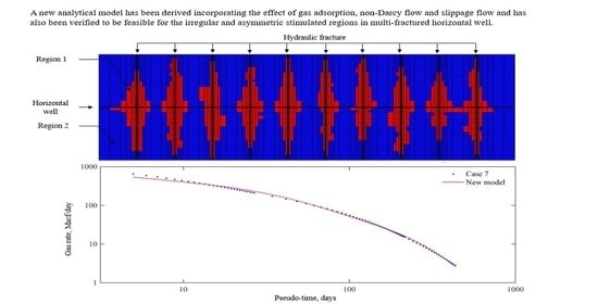
3.4. Irregular Stimulated Regions with Several Hydraulic Fractures

In order to further validate the applicability in irregular region of the new derived model, three more numerical cases of multifractured horizontal wells are designed, as shown in Figure 6. These three cases have the identical dimension with 163 grid cells in the x-direction, 63 grid cells in the y-direction, and only one grid cell of 10 ft in the z-direction. The length of the horizontal well is 762 ft with 10 hydraulic fractures equally spaced along the x-direction. For Case 5, the stimulated regions are all the same regular and symmetrical regions. As a comparison, the stimulated regions in Case 6 are all irregular but symmetrical regions. Meanwhile, there is no interference between fractures in Case 5 and Case 6 and the length of the hydraulic fractures is 352 ft in Case 5 and 464 ft in Case 6. As for Case 7, all the stimulated regions around each hydraulic fracture are different, irregular, and asymmetric. The length of 10 hydraulic fractures ranges from 288 to 432 ft and there is interference between fractures. The other input parameters are the same with Case 1.

Figure 7 shows the comparison of gas rate versus pseudo-time obtained from numerical simulations and the new analytical solutions. It can be seen that the results agree very well. Four regimes are also identified. The linear flow time in region 1 based on the fitting results is 9, 7, and 5 days for the three cases, respectively. Then it displays the boundary flow of region 1, which lasts until about the 100th day. The time constant in region 2 is 72, 79, and 91 days, respectively. Finally, the boundary flow of region 2 lasts for hundreds of days. We can obtain that the decline rate of gas production is faster during regimes 1 and 2 and thus the regimes 3 and 4 can last for a longer time. Therefore, for the shale gas reservoir, it is crucial to enhance the volume of stimulated regions to keep a longer high production period. Meanwhile, the contribution of gas adsorption mainly reflects in regimes 3 and 4. It helps to extend the stable production period. According to the output parameters after fitting with the numerical cases, we can calculate the volume of the hydraulic fracture region, region 1, and region 2, as shown in

Table 5. Inferred parameters value according to fitting results.

Case	τF	τ1	τ2	Tr21/Tr1F	Tr1F/J	qiF (Mscf/D)	Given Data (ft3)	Calculated Data (ft3)	Relative Error
Case 5	0.02	9	72	0.03	1.6	990	VpF = 21	VpF = 23	9.5%
							Vp1 = 106,022	Vp1 = 103,820	2.1%
							Vp2 = 105,281	Vp2 = 98,054	6.7%
Case 6	0.03	7	79	0.03	2.4	937	VpF = 28	VpF = 27	6.5%
							Vp1 = 81,062	Vp1 = 79,302	2.2%
							Vp2 = 130,234	Vp2 = 125,139	3.8%
Case 7	0.02	5	91	0.05	1.9	911	VpF = 24	VpF = 23	4.2%
							Vp1 = 67,264	Vp1 = 66,097	1.7%
							Vp2 = 144,036	Vp2 = 151,950	5.5%

. Considering that the relative errors meet the requirement of engineering accuracy, our new model is also suitable for the multifractured horizontal well.

3.5. Application to Field Case

The previous section demonstrated the accuracy of the derived analytical solution for production analysis. In this section, we apply the method to history matching and forecasting of field data in a shale gas reservoir. The gas well is selected for its relatively long production history and availability of pressure data. The main work flow is as follows:

• Apply the given parameters and gas material balance equation to transform the time into pseudo-time and pressure into pseudo-pressure.
• Make a diagnostic plot of production rate vs. pseudo-time.
• Analyze the diagnostic plot to identify flow regimes.
• Fit Equation (75) to the production data to obtain the model parameters τ_F, τ₁, τ₂, T_r21/T_r1F, T_r1F/J, and q_iF.
• Output the model parameters until a satisfactory matching is obtained.
• Following the step-by-step procedure to calculate the volume of hydraulic fracture region, region 1, and region 2.
• Make forecast of production rate with the model parameters.

We chose a horizontal well called Well B-15 with multiple fracture stages from Barnett shale [40]. The general data of the well for analysis is listed in

Table 6. Summary of the reservoir parameters for analysis.

Parameter	Value
Initial pressure (Psi)	2950
Bottom-hole pressure (Psi)	480
Temperature (K)	344.3
Langmuir volume (Scf/ton)	96
Langmuir pressure (Psi)	650
Compressibility (Psi−1)	4 × 10−6
Porosity	0.06

. The well was produced under constant pressure and even for short early variable p/q the constant pressure was also applicable [41]. Firstly, we transformed the time into pseudo-time and the relationship between pseudo-time and time is shown in Figure 8a. The plot of 1/q vs. square root pseudo-time for regime diagnosis is shown in Figure 8b. Then the log-log diagnostic plot of gas rate versus pseudo-time was obtained, which exhibits a half-slope straight line in Figure 8c. According to the previous analysis, the flow time in matrix is longer and the decline rate in region 2 is slower. Therefore, the half-slope linear flow was diagnosed as the regime 3. Following the work flow, the next step was to match our model to the production data. The results of history matching and forecasting is shown in Figure 8c. The red marks in Figure 8c represent the production data and the green ones represent the analytical solution for history matching. It indicates a good matching. The six model parameters obtained from history matching are summarized in

Table 7. Model parameters used in the analytical model for application in the field example.

Parameter	Value
τF (days)	0.01
τ1 (days)	11
τ2 (days)	3105
Tr21 / Tr1F	0.075
Tr1F / J	0.86
qiF (Mscf/D)	19,041

. Based on the parameters, we forecast the gas rate represented by the black markers in Figure 8c. According to the step-by-step procedure, we calculated the volume of the hydraulic fracture region as 89 ft³, the volume of stimulated region as 84.2 MMscf, and the volume of region 2 as 1784.2 MMscf. It is essential for increasing high production period by extending the volume of the stimulated region and decreasing the decline rate in the stimulated region.

4. Discussion

The results of this study can be summarized as four types: (1) derivation of the approximate analytical solution; (2) validation of the solution against different numerical models; (3) introducing a step-by-step procedure to predict the values of physical parameters; (4) application of the analytical model in the field case.

Result 1 is one of the novelty of the article. The model contains three regions and effectively accounts for non-Darcy flow in the hydraulic fractures, and gas adsorption and slippage in the matrix. During the derivation process, the governing PDEs are transformed into ordinary differential equations (ODEs) by integration, instead of the Laplace transform. There is no doubt that Laplace transform works extremely well. However, there are still some problems: (1) the first step for Laplace transform is dimensionless transformation. For some dimensionless variables such as dimensionless time, dimensionless pressure, dimensionless production, and so on, more inputs are needed and many are even estimated, which will lead to calculation error. (2) The numerical inversion is an essential step for converting Laplace space into real-time space. Among them, Stefest numerical inversion algorithm is most commonly used. In this algorithm, the number of inversion items $N$ is uncertain. The improper value will result in deviations in real time. Certainly, Result 1 also has some imperfections. For example, a dual-porosity model with Knudsen diffusion [6] would be more representative and the heterogeneity deserves further study.

Result 2 is the key section in the article. Seven numerical cases were set for verification. According to the fitting results, it shows that the analytical solution is feasible for the irregular and asymmetric stimulated regions in a multifractured horizontal well. Considering that the shapes of the enhanced fracture regions are unknown in real cases, we creatively set three types of stimulated regions: regular region, irregular region, and very irregular region. At least, the validation results show that our model is robust.

Result 3 is another novelty of our work. It introduced a step-by-step procedure to calculate inversion parameters. Comparing with the given volumes and calculated volumes from case 1 to case 7, the model is also verified to meet the engineering requirements. Considering the simplifying assumptions, the model may need to be improved and the accurate microseismic data would be required to make further verification.

Result 4 is the most important section. Considering the decline characteristics of shale gas, the constant rate case is not as important as the constant pressure case for long term performance of tight/shale formations. Therefore, our model is derived based on the constant bottom-hole pressure condition, and namely one of limitations for our model is that it cannot be applied in a constant rate case. The second limitation is the data continuity, because the prerequisite for the model to make accurate prediction is great fitting. As for the discontinuous data like data missing, shut-in, or pressure/production jump, our model is not applicable. Combined with the assumption of single-phase flow in this work, the multiphase flow problem cannot be solved by this analytical solution. Gas–water two-phase flow is the most common in shale gas reservoirs, so our future work is to derive the new analytical solution for gas–water two-phase flow.

5. Conclusions

In this paper, we presented a practical analytical model to study the performance of MFHWs from shale gas reservoirs. Numerical models have been used to validate the analytical solutions and an excellent agreement was obtained. The following conclusions are drawn from this work:

• A simple rate versus pseudo-time relationship is presented to account for transient linear and boundary-dominated flow periods in shale gas formation.
• Incorporating the effect of gas adsorption, non-Darcy flow, and slippage flow in the analytical model by defining the modified pseudo-pressure and pseudo-time, accuracy is improved in production forecast in shale gas reservoir.
• Comparing to the Laplace-transform solution, our analytical model is derived in real-time space and it is unnecessary to undertake dimensionless transformation and numerical inversion. It is more applicable in field scale.
• Through the model parameters obtained from history matching the field data, the production rate and cumulative production can be forecasted. In addition, the pore volume of different regions can also be calculated by step-by-step procedure, which was validated to be feasible for the irregular and asymmetric stimulated regions in multifractured horizontal wells. According to the results, the calculation accuracy is less than 10% and meets the engineering requirements.

References

1. Hu, X.Y.; Li, M.T.; Peng, C.G.; Davarpanah, A. Hybrid Thermal-Chemical Enhanced Oil Recovery Methods—An Experimental Study for Tight Reservoirs. Symmetry 2020, 12, 947. [Google Scholar] [CrossRef]
2. Jin, Y.; Davarpanah, A. Using Photo-Fenton and Floatation Techniques for the Sustainable Management of Flow-Back Produced Water Reuse in Shale Reservoirs Exploration. Water Air Soil Pollut. 2020, 231, 1–8. [Google Scholar] [CrossRef]
3. Hu, X.; Xie, J.; Cai, W.; Wang, R.; Davarpanah, A. Thermodynamic Effects of Cycling Carbon Dioxide Injectivity in Shale Reservoirs. J. Pet. Sci. Eng. 2020, 195, 107717. [Google Scholar] [CrossRef]
4. Wu, M.L.; Ding, M.C.; Yao, J.; Li, C.; Huang, Z.; Xu, S. Production-Performance Analysis of Composite Shale-Gas reservoirs by the Boundary-Element Method. SPE Reserv. Eval. Eng. 2019, 22, 238–252. [Google Scholar] [CrossRef] [Green Version]
5. Sun, S.H.; Zhou, M.H.; Lu, W.; Davarpanah, A. Application of Symmetry Law in Numerical Modeling of Hydraulic Fracturing by Finite Element Method. Symmetry 2020, 12, 1122. [Google Scholar] [CrossRef]
6. Sun, H.; Chawathe, A.; Hoteit, H.; Shi, X.; Li, L. Understanding Shale Gas Flow Behavior Using Numerical Simulation. SPE J. 2015, 20, 142–154. [Google Scholar] [CrossRef]
7. Zhang, M.; Sun, Q.; Ayala, L.F. Semi-Analytical Modeling of Multi-Mechanism Gas Transport in Shale Reservoirs with Complex Hydraulic-Fracture Geometries by the Boundary Element Method. In Proceedings of the SPE Annual Technical Conference and Exhibition, Calgary, AB, Canada, 30 September–2 October 2019. SPE Paper 195902-MS. [Google Scholar]
8. Davarpanah, A.; Shirmohammadi, R.; Mirshekari, B.; Aslani, A. Analysis of hydraulic fracturing techniques: Hybrid fuzzy approaches. Arab. J. Geosci. 2019, 12, 402. [Google Scholar] [CrossRef]
9. Nobakht, M.; Clarkson, C.R. A New Analytical Method for Analyzing Linear Flow in Tight/Shale Gas Reservoirs: Constant-Flowing-Pressure Boundary Condition. SPE Reserv. Eval. Eng. 2012, 15, 370–384. [Google Scholar] [CrossRef] [Green Version]
10. Zhao, Y.L.; Zhang, L.H.; Luo, J.X.; Zhang, B.-N. Performance of fractured horizontal well with stimulated reservoir volume in unconventional gas reservoir. J. Hydrol. 2014, 512, 447–456. [Google Scholar] [CrossRef]
11. Clarkson, C.R.; Qanbari, F. An Approximate Semianalytical Multiphase Forecasting Method for Multifractured Tight Light-Oil Wells With Complex Fracture Geometry. J. Can. Pet. Technol. 2015, 54, 489–508. [Google Scholar] [CrossRef]
12. Wei, S.M.; Xia, Y.; Jin, Y. Quantitative study in shale gas behaviors using a coupled triple-continuum and discrete fracture model. J. Pet. Sci. Eng. 2019, 174, 49–69. [Google Scholar] [CrossRef]
13. Wang, Q.; Wan, J.F.; Mu, L.F.; Shen, R.; Jurado, M.J.; Ye, Y. An Analytical Solution for Transient Productivity Prediction of Multi-Fractured Horizontal Wells in Tight Gas Reservoirs Considering Nonlinear Porous Flow Mechanisms. Energies 2020, 13, 1066. [Google Scholar] [CrossRef] [Green Version]
14. Zhang, Q.; Jiang, S.; Wu, X.Y. Development and Calibration of a Semianalytic Model for Shale Wells with Nonuniform Distribution of Induced Fractures Based on ES-MDA Method. Energies 2020, 13, 3718. [Google Scholar] [CrossRef]
15. Lee, S.T.; Brockenbrough, J. A New Analytic Solution for Finite Conductivity Vertical Fractures With Real Time and Laplace Space Parameter Estimation. In Proceedings of the SPE Annual Technical Conference and Exhibition, San Francisco, CA, USA, 5–8 October 1983. SPE Paper 12013-MS. [Google Scholar]
16. Wattenbarger, R.A.; El-Banbi, A.H.; Villegas, M.E.; Maggard, J.B. Production Analysis of Linear Flow into Fractured Tight Gas Wells. In Proceedings of the SPE Rocky Mountain Regional/Low-Permeability Reservoirs Symposium, Denver, CO, USA, 5–8 April 1998. SPE Paper 39931-MS. [Google Scholar]
17. El-Banbi, A.H.; Wattenbarger, R.A. Analysis of Linear Flow in Gas Well Production. In Proceedings of the SPE Gas Technology Symposium, Calgary, AB, Canada, 15–18 March 1998. SPE Paper 39972-MS. [Google Scholar]
18. Bello, R.O.; Wattenbarger, R.A. Multi-Stage Hydraulically Fractured Horizontal Shale Gas Well Rate Transient Analysis. In Proceedings of the North Africa Technical Conference and Exhibition, Cairo, Egypt, 14–17 February 2010. SPE Paper 126754-MS. [Google Scholar]
19. Ozkan, E.; Brown, M.L.; Raghavan, R.S.; Kazemi, H. Comparison of Fractured Horizontal-Well Performance in Conventional and Unconventional Reservoirs. In Proceedings of the SPE Western Regional Meeting, San Jose, CA, USA, 24–26 March 2009. SPE Paper 121290-MS. [Google Scholar]
20. Brown, M.; Ozkan, E.; Raghavan, R.; Kazemi, H. Practical Solutions for Pressure-Transient Responses of Fractured Horizontal Wells in Unconventional Shale Reservoirs. SPE Reserv. Eval. Eng. 2011, 14, 663–676. [Google Scholar] [CrossRef]
21. Stalgorova, E.; Mattar, L. Practical Analytical Model to Simulate Production of Horizontal Wells with Branch Fractures. In Proceedings of the SPE Canadian Unconventional Resources Conference, Calgary, AB, Canada, 30 October–1 November 2012. SPE Paper 162515-MS. [Google Scholar]
22. Heidari, S.M.; Clarkson, C.R. An Analytical Model for Analyzing and Forecasting Production from Multi-fractured Horizontal Wells with Complex Branched-Fracture Geometry. SPE Reserv. Eval. Eng. 2015, 18, 356–374. [Google Scholar] [CrossRef]
23. Abassi, M.; Sharifi, M.; Kazemi, A. Development of New Analytical Model for Series and Parallel Triple Porosity Models and Providing Transient Shape Factor between Different Regions. J. Hydrol. 2019, 574, 683–698. [Google Scholar] [CrossRef]
24. Yao, F. Production Evaluation of Fracturing Horizontal Wells for Solution Gas Drive in Tight Oil Reservoirs; China University of Petroleum (Beijing): Beijing, China, 2018. [Google Scholar]
25. Stehfest, H. Algorithm 368: Numerical inversion of Laplace transforms [D5]. Commun. ACM 1970, 13, 47–49. [Google Scholar] [CrossRef]
26. Shahamat, M.S.; Mattar, L.; Aguilera, R. A Physics-Based Method for Production Data Analysis of Tight and Shale Petroleum Reservoirs Using Succession of Pseudo-Steady States. In Proceedings of the SPE/EAGE European Unconventional Resources Conference and Exhibition, Vienna, Austria, 25–27 February 2014. SPE Paper 167686-MS. [Google Scholar]
27. Ogunyomi, B.A. Simple Mechanistic Modeling of Recovery from Unconventional Oil Reservoirs; The University of Texas at Austin: College Station, TX, USA, 2015. [Google Scholar]
28. Ogunyomi, B.A.; Patzek, T.W.; Lake, L.W.; Kabir, C.S. History Matching and Rate Forecasting in Unconventional Oil Reservoirs With an Approximate Analytical Solution to the Double-Porosity Model. SPE Reserv. Eval. Eng. 2016, 19, 70–82. [Google Scholar] [CrossRef]
29. Qiu, K.X.; Li, H. A New Analytical Solution of the Triple-Porosity Model for History Matching and Performance Forecasting in Unconventional Oil Reservoirs. SPE J. 2018, 23, 2060–2079. [Google Scholar] [CrossRef]
30. Qiu, K.X.; Li, H. A New Analytical Model for Production Forecasting in Unconventional Reservior Considering the Simultaneous Matrix-fracture flow. In Proceedings of the Asia Pacific Unconventional Resource Technology Conference, Brisbane, Australia, 18–19 November 2019. SPE Paper URTEC-198266-MS. [Google Scholar]
31. Tabatabaie, S.H. Unconventional Reservoirs: Mathematical Modeling of Some Non-linear Problems; University of Calgary: College Station, AB, Canada, 2014. [Google Scholar]
32. Behmanesh, H.; Hamdi, H.; Clarkson, C.R.; Thompson, J.M.; Anderson, D.M. Analytical Modeling of Linear Flow in Single-Phase Tight Oil and Tight Gas Reservoirs. J. Pet. Sci. Eng. 2018, 171, 1084–1098. [Google Scholar] [CrossRef]
33. Anderson, D.M.; Nobakht, M.; Moghadam, S.; Mattar, L. Analysis of Production Data from Fractured Shale Gas Wells. In Proceedings of the SPE Unconventional Gas Conference, Pittsburgh, PA, USA, 23–25 February 2010. SPE Paper 131787. [Google Scholar]
34. Langmuir, I. The Constitution and Fundamental Properties of Solids and Liquids. J. Am. Chem. Soc. 1916, 38, 2221–2295. [Google Scholar] [CrossRef] [Green Version]
35. Bumb, A.C.; McKee, C.R. Gas-Well Testing in the Presence of Desorption for Coal bed Methane and Devonian Shale. In Proceedings of the SPE Unconventional Gas Technology Symposium, Louisville, KY, USA, 18–21 May 1986. SPE Paper 15227-MS. [Google Scholar]
36. King, G.R. Material Balance Techniques for Coal Seam and Devonian Shale Gas Reservoirs. In Proceedings of the SPE Annual Technical Conference and Exhibition, New Orleans, Louisiana, 23–26 September 1990. SPE Paper 20730-MS. [Google Scholar]
37. Forchheimer, P. Wasserbewegung Durch Boden. Z. Ver. Deutsch Ing. 1901, 45, 1782–1788. [Google Scholar]
38. Wang, J.; Lou, H.S.; Liu, H.Q. An Intergrative Model to Simulate Gas Transport and Production Coupled With Gas Adsorption, Non-Darcy Flow, Surface Diffusion, and Stress Dependence in Organic-Shale Reservoir. SPE J. 2017, 22, 244–264. [Google Scholar] [CrossRef]
39. Wang, H.Y.; Porcu, M.M. Impact of Shale-Gas Apparent Permeability on Production: Combined Effects of Non-Darcy Flow/Gas Slippage, Desorption and Geomechanics. SPE Reserv. Eval. Eng. 2015, 18, 495–507. [Google Scholar] [CrossRef]
40. Samandarli, O. A New Method for History Matching and Forecasting Shale Gas/Oil Reservoir Production Performance with Dual and Triple Porosity Models; Texas A&M University: College Station, TX, USA, 2011. [Google Scholar]
41. Hamdi, H.; Behmanesh, H.; Clarkson, C.R. A Semi-Analytical Approach for Analysis of Wells Exhibiting Multi-Phase Transient Linear Flow: Application to Field Data. In Proceedings of the SPE Annual Technical Conference and Exhibition, Calgary, AB, Canada, 30 September–2 October 2019. SPE Paper 196164-MS. [Google Scholar]
Figure 1. Schematic of a multistage fractured horizontal well with two regions around the hydraulic fracture. (a) The 3D model. (b) The plan view.
Energies 13 05899 g001
Figure 2. Reservoir grid for the numerical model. The red grids are the high-permeability region and the blue ones are the low-permeability region.
Energies 13 05899 g002
Figure 3. The result analysis for Case 1. (a) Comparison of the relationship between pseudo-time and time. (b) The plot 1/q vs. square root pseudo-time for regime diagnosis. (c) Comparison of the relationship between gas rate and pseudo-time. (Regime 1: transient linear flow in region 1 with slope -1/2. Regime 2: boundary-dominated flow for region 1. Regime 3: transient linear flow in region 2 with slope -1/2. Regime 4: boundary-dominated flow for region 2).
Energies 13 05899 g003
Figure 4. Reservoir grid for the numerical cases showing different shapes of stimulated region. The red grids are the stimulated region and the blue ones are the low-permeability region.
Energies 13 05899 g004
Figure 5. Comparison of the relationship of gas rate vs. pseudo-time from the numerical cases and new analytical solution. (a) Comparison of the relationship of gas rate vs. pseudo-time from the Case 2 and new model. (b) Comparison of the relationship of gas rate vs. pseudo-time from the Case 3 and new model. (c) Comparison of the relationship of gas rate vs. pseudo-time from the Case 4 and new model.
Energies 13 05899 g005
Figure 6. Reservoir grid for multifractured horizontal well (MFHWs).
Energies 13 05899 g006
Figure 7. Comparison of the relationship of gas rate vs. pseudo-time from the numerical cases and new analytical solution. (a) Comparison of the relationship of gas rate vs. pseudo-time from the Case 5 and new model. (b) Comparison of the relationship of gas rate vs. pseudo-time from the Case 6 and new model. (c) Comparison of the relationship of gas rate vs. pseudo-time from the Case 7 and new model.
Energies 13 05899 g007
Figure 8. Summary of production profiles for the field example. (a) The relationship between time and pseudo-time. (b) The plot 1/q vs. square root pseudo-time for regime diagnosis. (c) The results of history-matching and forecasting on log-log plot.
Energies 13 05899 g008