Forecasting Electricity Consumption in Commercial Buildings Using a Machine Learning Approach


Abstract

1. Introduction
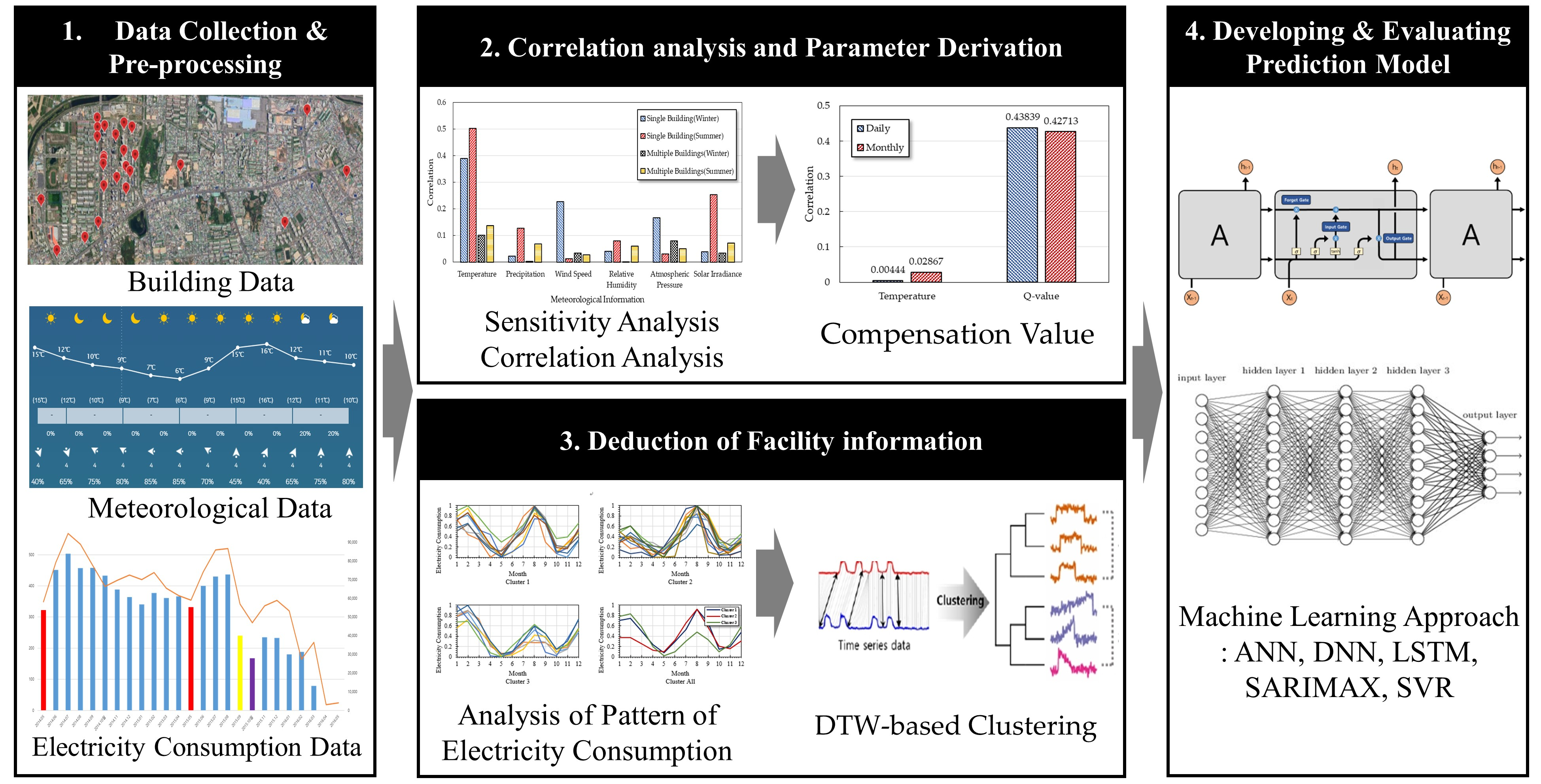
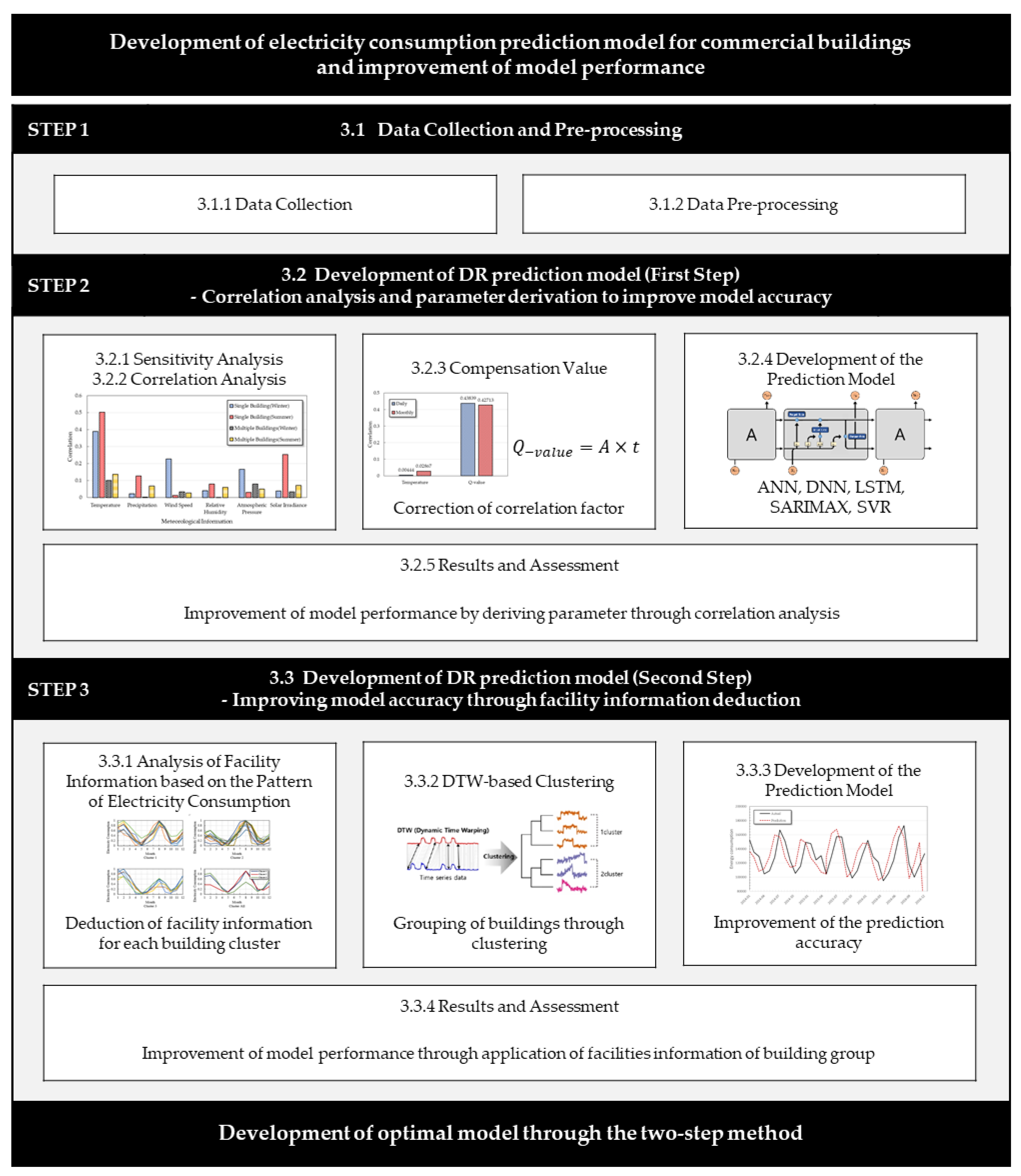
2. Research Framework
Literature Review
3. Method
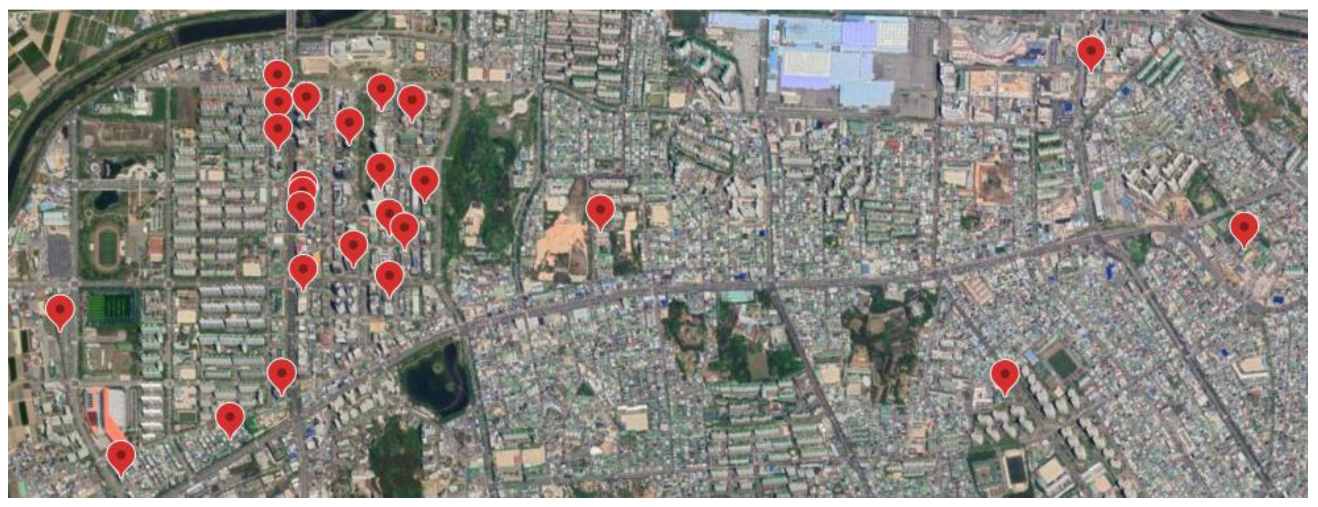
3.1. STEP 1: Data Collection and Pre-Processing
3.1.1. Data Collection
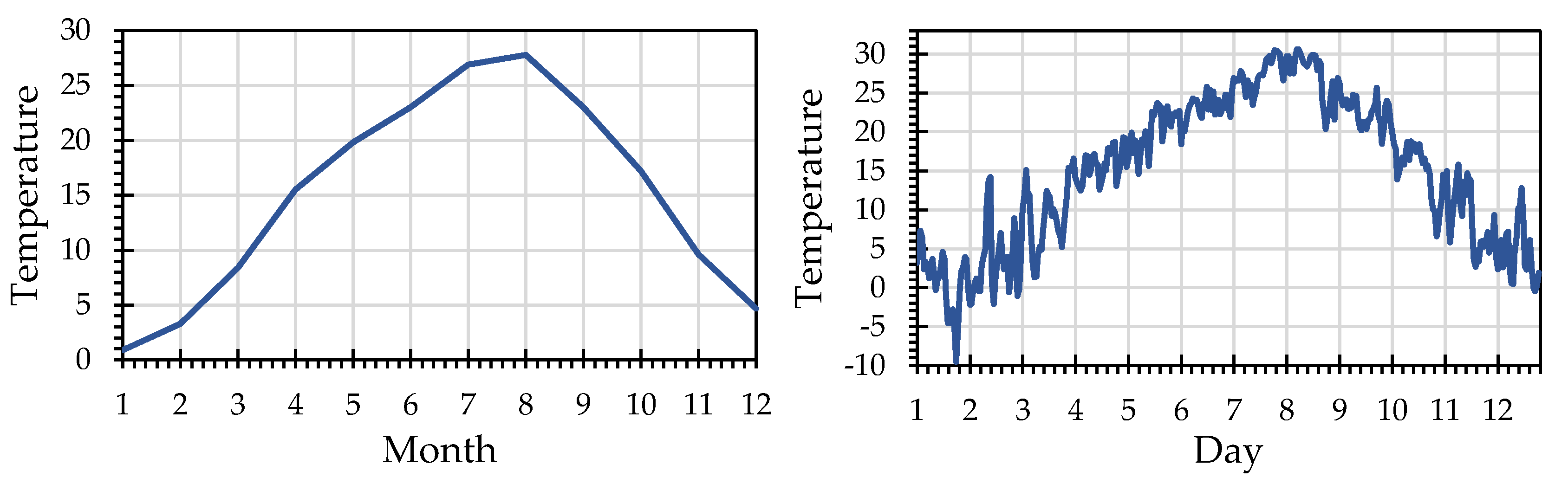
3.1.2. Pre-Processing
3.2. STEP 2: Development of DR Prediction Model (First Step)
3.2.1. Sensitivity Analysis
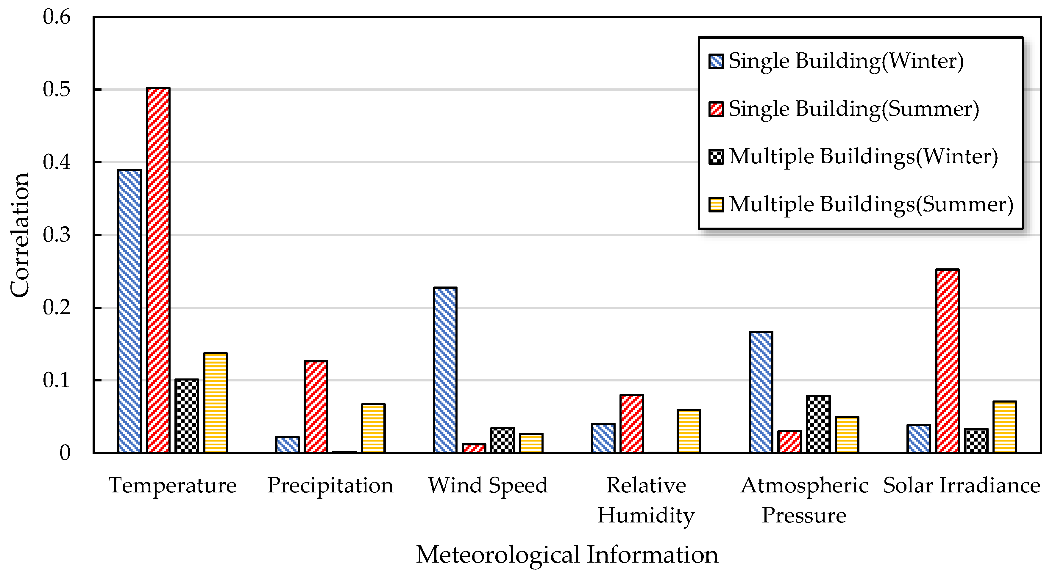
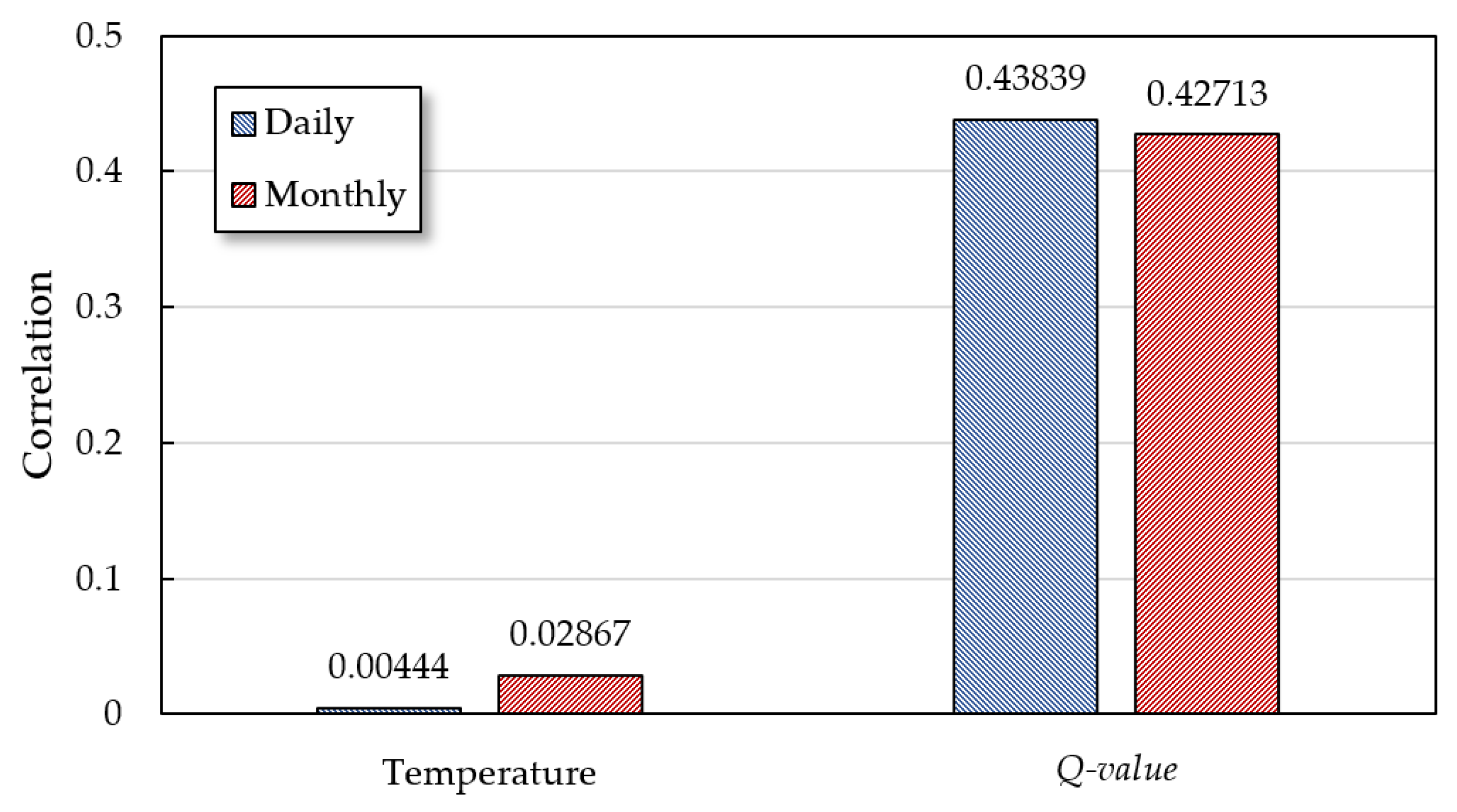
3.2.2. Correlation Analysis
3.2.3. Compensation Value
3.2.4. Development of the Prediction Model (First Step)
- ANN
- SVR
- SARIMAX
- DNN
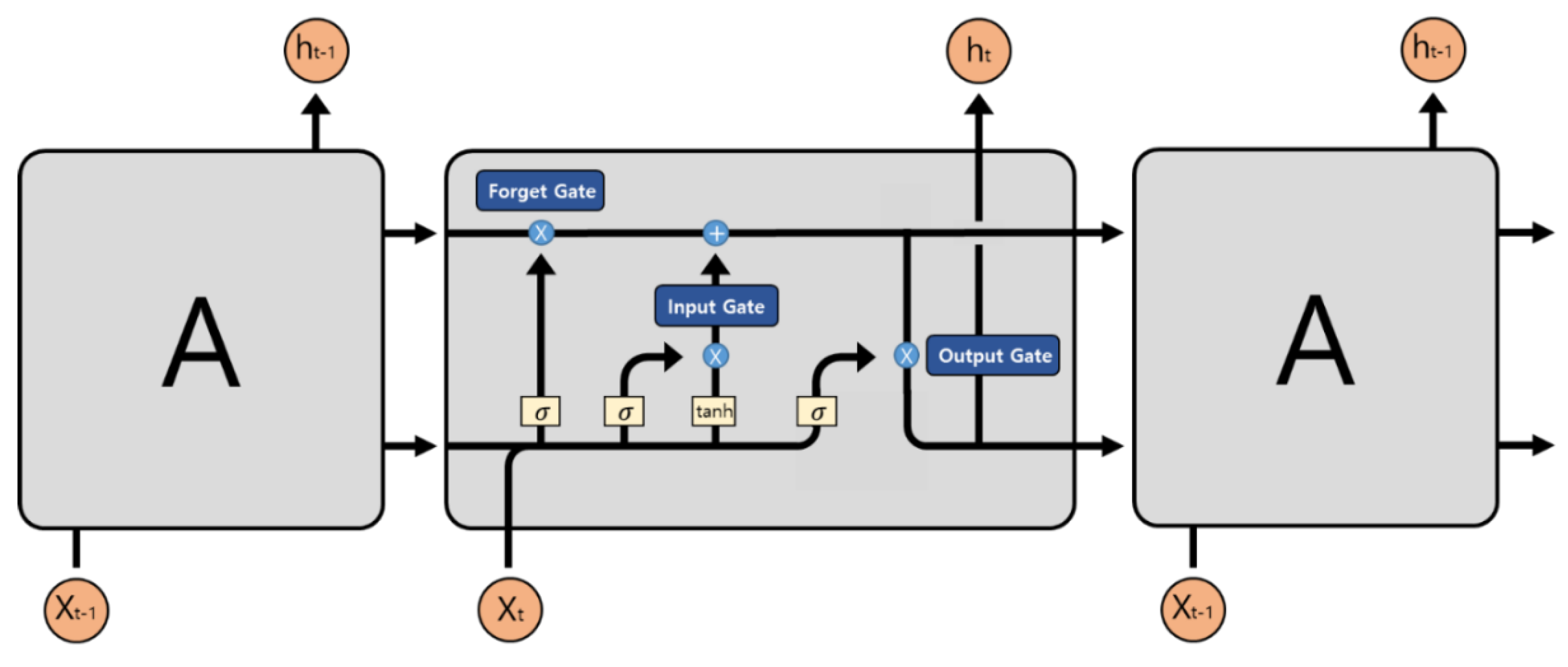
- LSTM
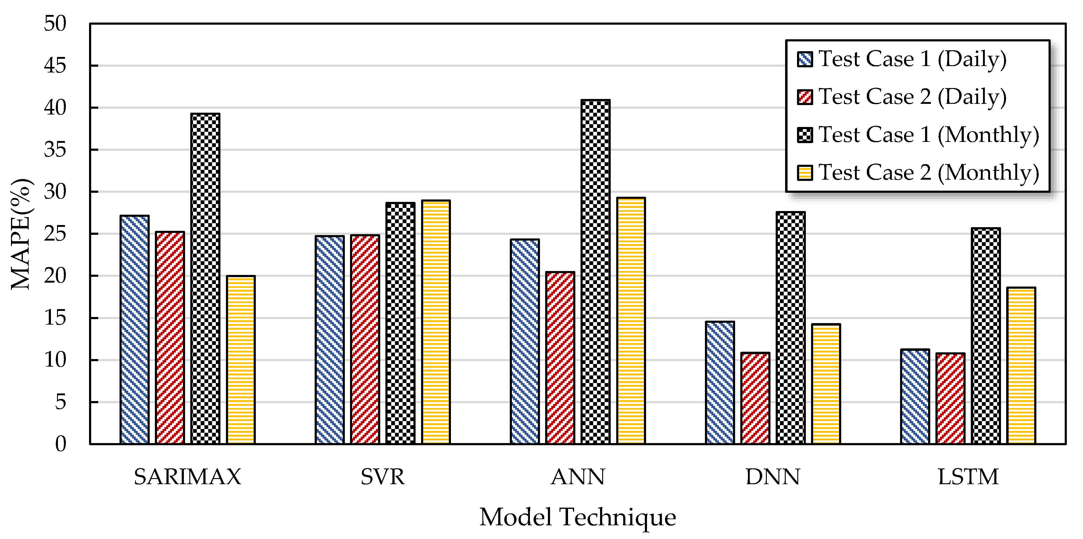
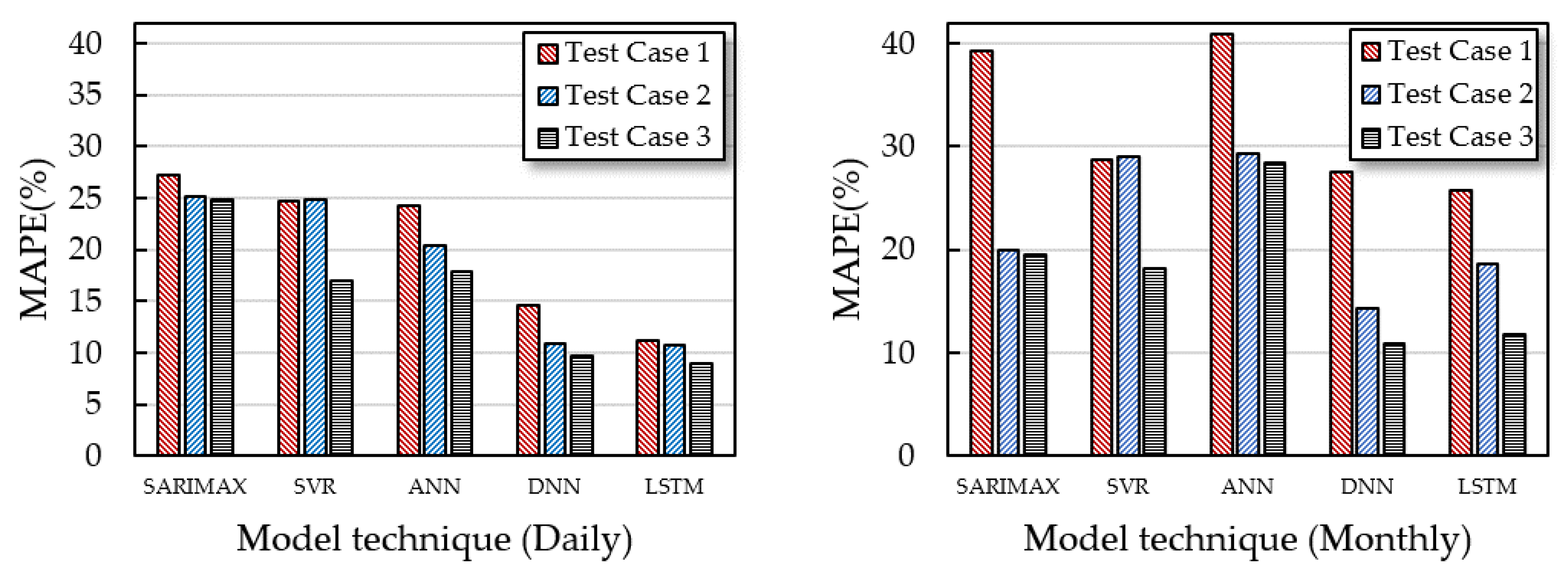
3.2.5. Results and assessment (First Step)
- Error calculation
- Assessment of trained models
3.3. STEP 3: Development of DR Prediction Model (Second Step)
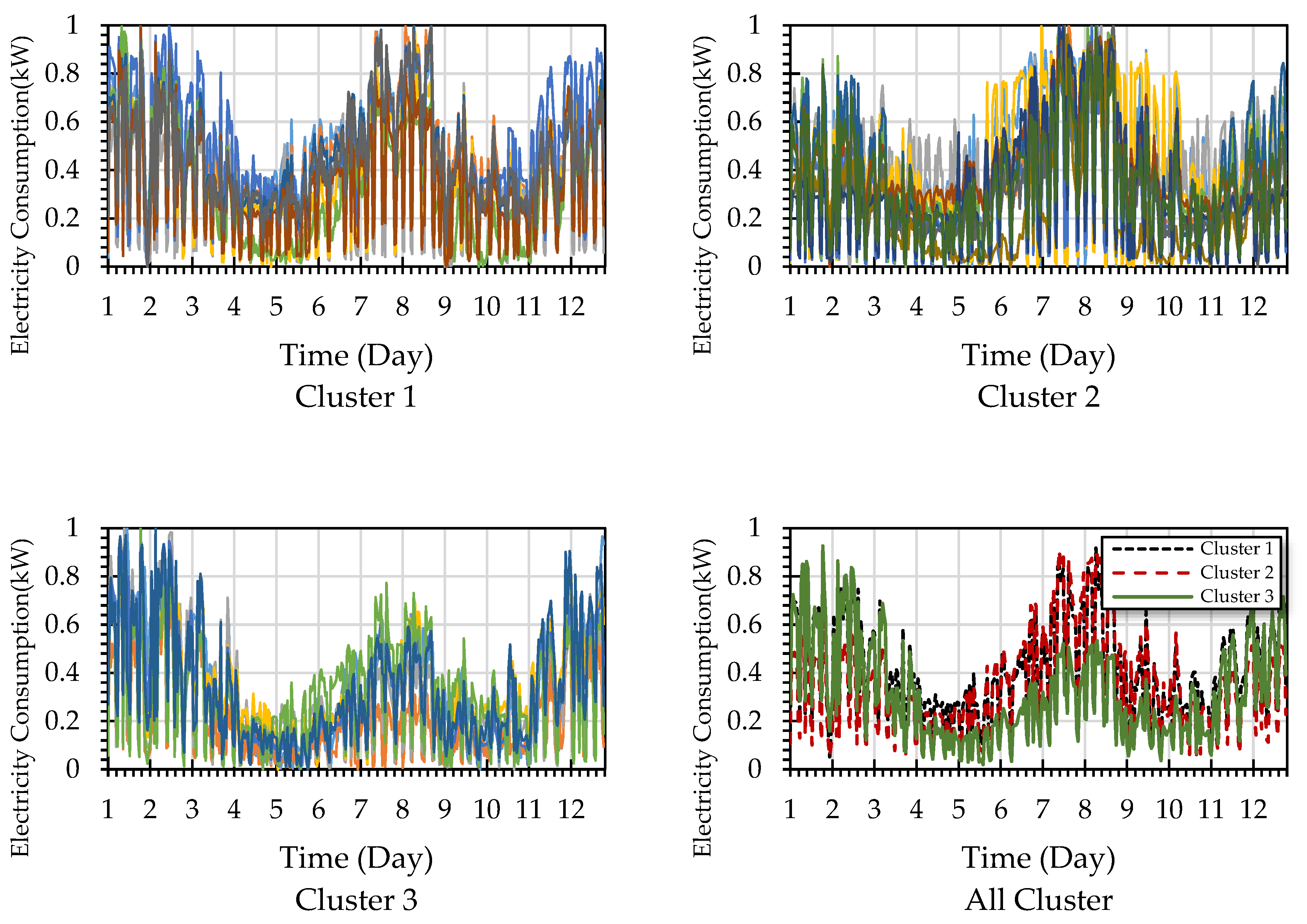
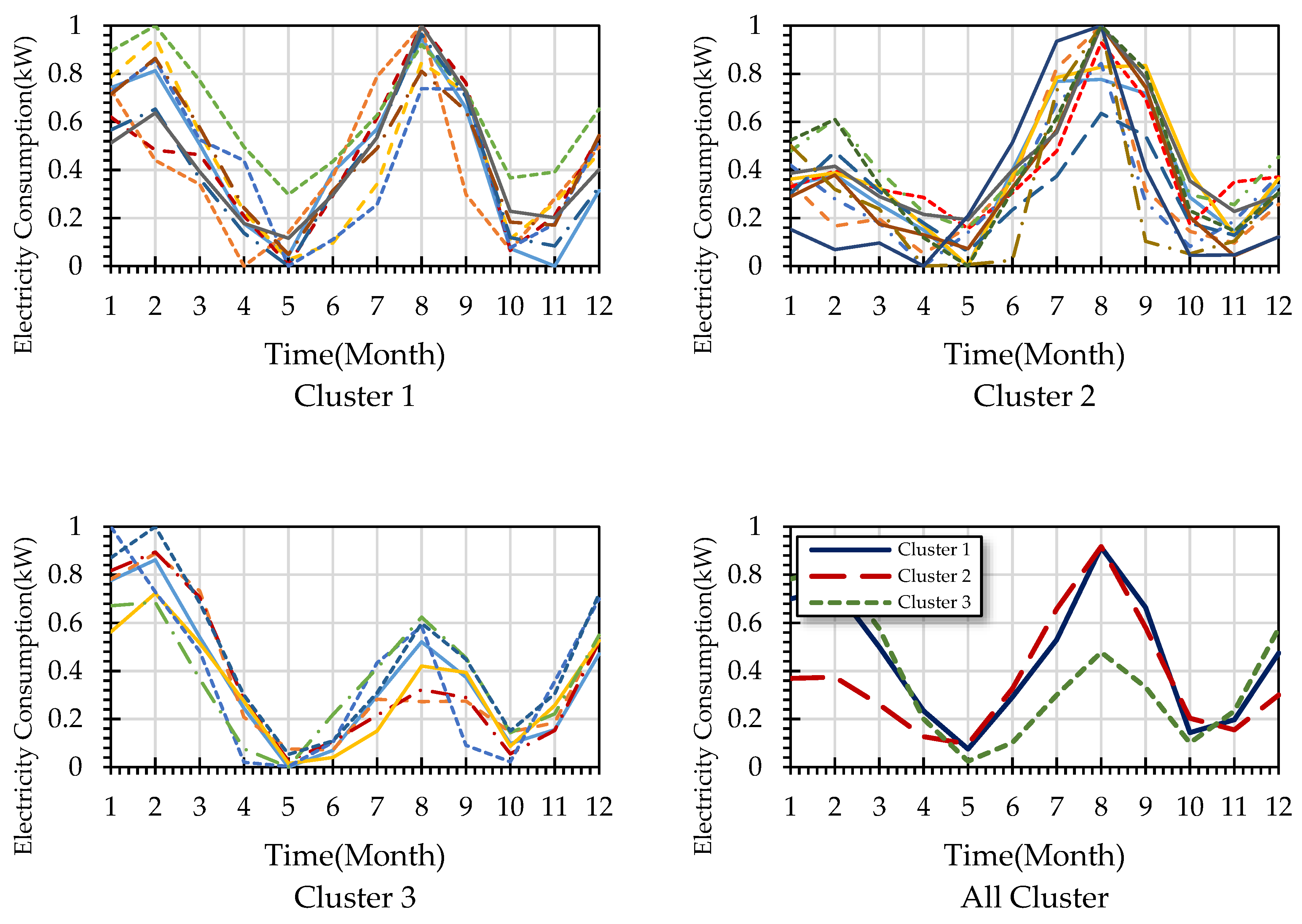
3.3.1. Analysis of Facility Information Based on the Pattern of Electricity Consumption
3.3.2. DTW-Based Clustering
3.3.3. Development of a Prediction Model (Second Step)
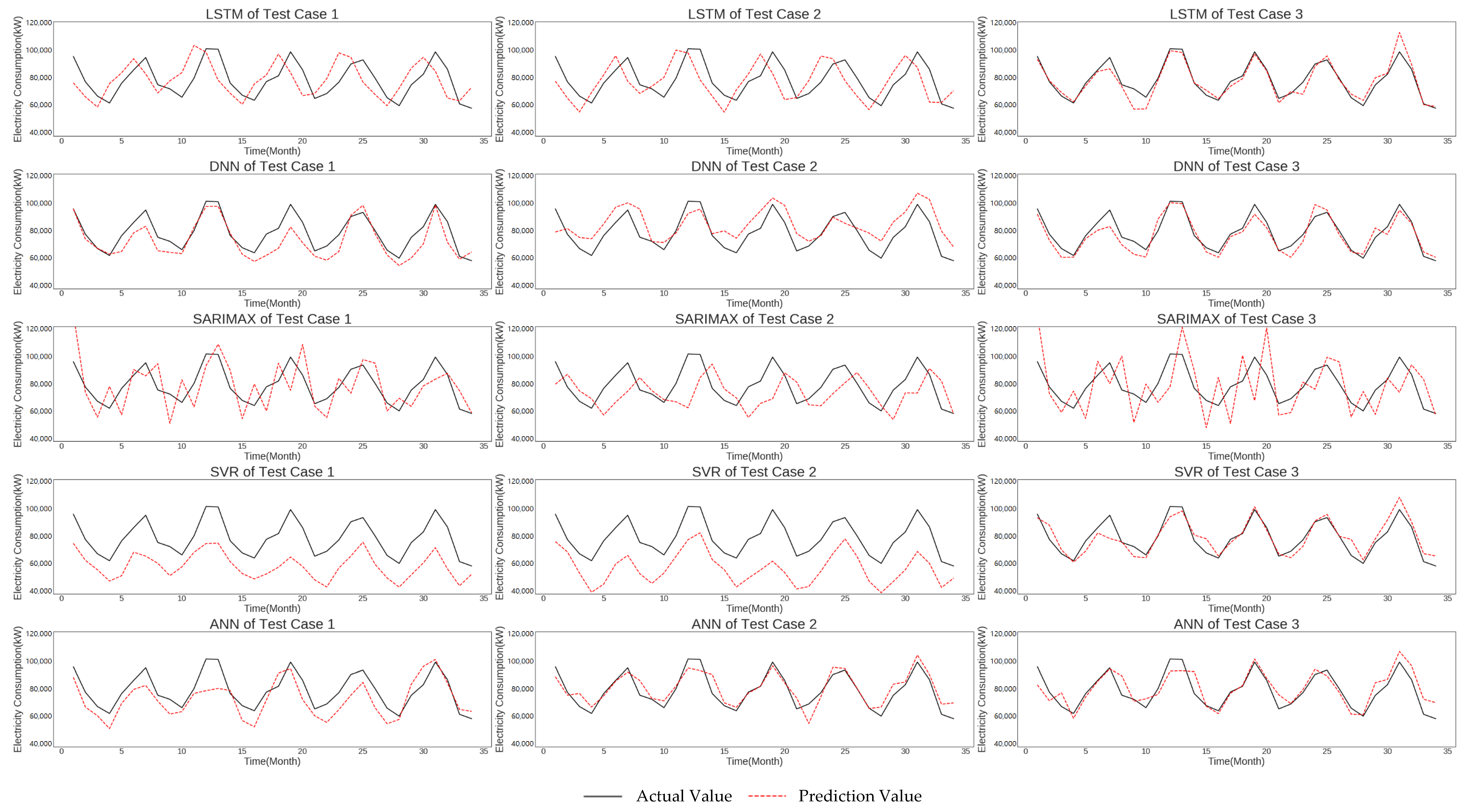
3.3.4. Results and Assessment (Second Step)
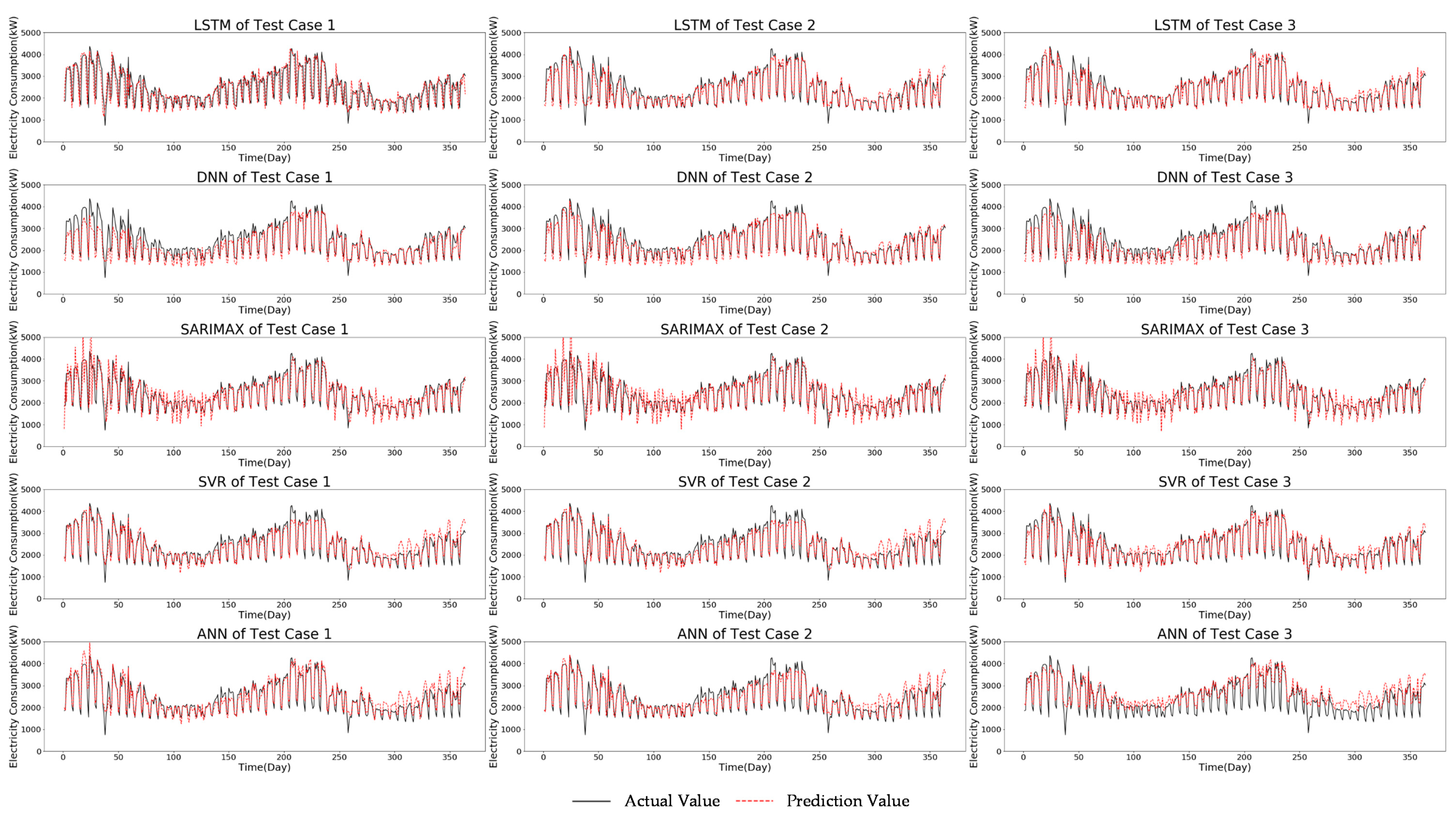
- Comparison of actual and predicted values
4. Discussion and Conclusions
Author Contributions
Funding
Conflicts of Interest
References
- Cullen, D. Climate change. Nature 2011, 479, 267–268. [Google Scholar] [CrossRef]
- Horowitz, C.A. Paris Agreement. Int. Leg. Mater. 2016, 55, 740–755. [Google Scholar] [CrossRef]
- Bae, K.Y.; Jang, H.S.; Jung, B.C.; Sung, D.K. Effect of Prediction Error of Machine Learning Schemes on Photovoltaic Power Trading Based on Energy Storage Systems. Energies 2019, 12, 1249. [Google Scholar] [CrossRef]
- Kneifel, J.; Webb, D. Predicting energy performance of a net-zero energy building: A statistical approach. Appl. Energy 2016, 178, 468–483. [Google Scholar] [CrossRef]
- Walker, S.; Labeodan, T.; Boxem, G.; Maassen, W.; Zeiler, W. An assessment methodology of sustainable energy transition scenarios for realizing energy neutral neighborhoods. Appl. Energy 2018, 228, 2346–2360. [Google Scholar] [CrossRef]
- Kwon, O.S.; Bin Song, K. Development of Short-Term Load Forecasting Method by Analysis of Load Characteristics during Chuseok Holiday. Trans. Korean Inst. Electr. Eng. 2011, 60, 2215–2220. [Google Scholar] [CrossRef]
- Saleh, M.S.; Althaibani, A.; Esa, Y.; Mhandi, Y.; Mohamed, A.A. Impact of clustering microgrids on their stability and resilience during blackouts. In Proceedings of the 2015 International Conference on Smart Grid and Clean Energy Technologies (ICSGCE), Offenburg, Germany, 20–23 October 2015; pp. 195–200. [Google Scholar]
- Jeong, K.; Koo, C.; Hong, T. An estimation model for determining the annual energy cost budget in educational facilities using SARIMA (seasonal autoregressive integrated moving average) and ANN (artificial neural network). Energy 2014, 71, 71–79. [Google Scholar] [CrossRef]
- Muralitharan, K.; Sakthivel, R.; Vishnuvarthan, R. Neural network based optimization approach for energy demand prediction in smart grid. Neurocomputing 2018, 273, 199–208. [Google Scholar] [CrossRef]
- Ahmad, T.; Chen, H. Potential of three variant machine-learning models for forecasting district level medium-term and long-term energy demand in smart grid environment. Energy 2018, 160, 1008–1020. [Google Scholar] [CrossRef]
- Building Act. Korea Law Information Center. Available online: http://www.law.go.kr/법령/건축법 (accessed on 20 September 2020).
- Statistics on Buildings. Molit Statistics System. 2019. Available online: https://stat.molit.go.kr/ (accessed on 20 September 2020).
- Walker, S.; Khan, W.; Katic, K.; Maassen, W.; Zeiler, W. Accuracy of different machine learning algorithms and added-value of predicting aggregated-level energy performance of commercial buildings. Energy Build. 2020, 209, 109705. [Google Scholar] [CrossRef]
- Chae, Y.T.; Horesh, R.; Hwang, Y.; Lee, Y.M. Artificial neural network model for forecasting sub-hourly electricity usage in commercial buildings. Energy Build. 2016, 111, 184–194. [Google Scholar] [CrossRef]
- Ryu, S.; Noh, J.; Kim, H. Deep Neural Network Based Demand Side Short Term Load Forecasting. Energies 2016, 10, 3. [Google Scholar] [CrossRef]
- Rahman, A.; Srikumar, V.; Smith, A.D. Predicting electricity consumption for commercial and residential buildings using deep recurrent neural networks. Appl. Energy 2018, 212, 372–385. [Google Scholar] [CrossRef]
- Jain, R.; Smith, K.M.; Culligan, P.J.; Taylor, J.E. Forecasting energy consumption of multi-family residential buildings using support vector regression: Investigating the impact of temporal and spatial monitoring granularity on performance accuracy. Appl. Energy 2014, 123, 168–178. [Google Scholar] [CrossRef]
- Song, X.; Liu, Y.; Xue, L.; Wang, J.; Zhang, J.; Wang, J.; Jiang, L.; Cheng, Z. Time-series well performance prediction based on Long Short-Term Memory (LSTM) neural network model. J. Pet. Sci. Eng. 2020, 186, 106682. [Google Scholar] [CrossRef]
- Shao, M.; Wang, X.; Bu, Z.; Chen, X.; Wang, Y. Prediction of energy consumption in hotel buildings via support vector machines. Sustain. Cities Soc. 2020, 57, 102128. [Google Scholar] [CrossRef]
- Bouktif, S.; Fiaz, A.; Ouni, A.; Serhani, M.A. Optimal Deep Learning LSTM Model for Electric Load Forecasting using Feature Selection and Genetic Algorithm: Comparison with Machine Learning Approaches. Energies 2018, 11, 1636. [Google Scholar] [CrossRef]
- Ngo, N.-T. Early predicting cooling loads for energy-efficient design in office buildings by machine learning. Energy Build. 2019, 182, 264–273. [Google Scholar] [CrossRef]
- Choi, D.; Lee, Y.; Koh, M. The Prediction and Valuation of Gas Consumption in Building using Artificial Neural Networks Based on Clustering Method. KIEAE J. 2018, 18, 69–74. [Google Scholar] [CrossRef]
- Lee, Y.-J.; Ko, M.-J.; Choi, D.-S. Pattern and Energy Intensity Analysis of Monthly Gas Energy Consumption in Apartment Using Dynamic Time Warping Hierarchical Clustering. J. Korean Soc. Living Environ. Syst. 2019, 26, 134–139. [Google Scholar] [CrossRef]
- Pyle, D. Data Preparation for Data Mining; Morgan Kaufmann Publishers: Burlington, MA, USA, 1999. [Google Scholar]
- Bourdeau, M.; Zhai, X.; Nefzaoui, E.; Guo, X.; Chatellier, P. Modeling and forecasting building energy consumption: A review of data-driven techniques. Sustain. Cities Soc. 2019, 48. [Google Scholar] [CrossRef]
- Public Open Data. Available online: https://www.data.go.kr/ (accessed on 20 September 2020).
- Korea Meteorological Administration (KMA). Available online: https://data.kma.go.kr (accessed on 20 September 2020).
- A Legister of Building. Saeumteo. Available online: https://cloud.eais.go.kr (accessed on 20 September 2020).
- Meijering, E. A chronology of interpolation: From ancient astronomy to modern signal and image processing. Proc. IEEE 2002, 90, 319–342. [Google Scholar] [CrossRef]
- Ioffe, S.; Szegedy, C. Batch Normalization: Accelerating Deep Network Training by Reducing Internal Covariate Shift. Available online: https://arxiv.org/abs/1502.03167 (accessed on 20 September 2020).
- Sobol, I. Global sensitivity indices for nonlinear mathematical models and their Monte Carlo estimates. Math. Comput. Simul. 2001, 55, 271–280. [Google Scholar] [CrossRef]
- Wei, P.; Lu, Z.; Yuan, X. Monte Carlo simulation for moment-independent sensitivity analysis. Reliab. Eng. Syst. Saf. 2013, 110, 60–67. [Google Scholar] [CrossRef]
- Wei, P.; Lu, Z.; Song, J. Moment-Independent Sensitivity Analysis Using Copula. Risk Anal. 2013, 34, 210–222. [Google Scholar] [CrossRef]
- Borgonovo, E. A new uncertainty importance measure. Reliab. Eng. Syst. Saf. 2007, 92, 771–784. [Google Scholar] [CrossRef]
- Adler, J.; Parmryd, I. Quantifying colocalization by correlation: The pearson correlation coefficient is superior to the Mander’s overlap coefficient. Cytom. Part A 2010, 77A, 733–742. [Google Scholar] [CrossRef]
- McCulloch, W.S.; Pitts, W. A logical calculus of the ideas immanent in nervous activity. 1943. Assoc. Symb. Log 1990, 52, 99. [Google Scholar]
- Gurney, K. An Introduction to Neural Networks; CRC Press: Boca Raton, FL, USA, 2018. [Google Scholar]
- Cortes, C.; Vapnik, V. Support-vector networks. Mach. Learn. 1995, 20, 273–297. [Google Scholar] [CrossRef]
- Dong, B.; Cao, C.; Lee, S.E. Applying support vector machines to predict building energy consumption in tropical region. Energy Build. 2005, 37, 545–553. [Google Scholar] [CrossRef]
- Box, G.E.; Jenkins, G.M.; Reinsel, G.C.; Ljung, G.M. Time Series Analysis: Forecasting and Control; Wiley: Hoboken, NJ, USA, 2016. [Google Scholar]
- Contreras, J.; Espínola, R.; Nogales, F.J.; Conejo, A.J. ARIMA models to predict next-day electricity prices. IEEE Trans. Power Syst. 2003, 18, 1014–1020. [Google Scholar] [CrossRef]
- Bengio, Y.; Courville, A.; Vincent, P. Representation Learning: A Review and New Perspectives. IEEE Trans. Pattern Anal. Mach. Intell. 2013, 35, 1798–1828. [Google Scholar] [CrossRef] [PubMed]
- Hinton, G.; Deng, L.; Yu, D.; Dahl, G.E.; Mohamed, A.-R.; Jaitly, N.; Senior, A.; Vanhoucke, V.; Nguyen, P.; Sainath, T.N.; et al. Deep Neural Networks for Acoustic Modeling in Speech Recognition: The Shared Views of Four Research Groups. IEEE Signal Process. Mag. 2012, 29, 82–97. [Google Scholar] [CrossRef]
- Greff, K.; Srivastava, R.K.; Koutnik, J.; Steunebrink, B.R.; Schmidhuber, J. LSTM: A Search Space Odyssey. IEEE Trans. Neural Netw. Learn. Syst. 2016, 28, 2222–2232. [Google Scholar] [CrossRef]
- De Myttenaere, A.; Golden, B.; Le Grand, B.; Rossi, F. Mean Absolute Percentage Error for regression models. Neurocomputing 2016, 192, 38–48. [Google Scholar] [CrossRef]
- Hyndman, R.J.; Koehler, A.B. Another look at measures of forecast accuracy. Int. J. Forecast. 2006, 22, 679–688. [Google Scholar] [CrossRef]
- Stone, R. Improved statistical procedure for the evaluation of solar radiation estimation models. Sol. Energy 1993, 51, 289–291. [Google Scholar] [CrossRef]
- Son, C.-H.; Yang, I.-H. A Study on the Effect of Envelope Factors on Cooling, Heating and Lighting Energy Consumption in Office Building. J. Korean Inst. Illum. Electr. Install. Eng. 2012, 26, 8–17. [Google Scholar]
- Jung, S. A Study on the Comparison of Maximum Power Demand in Building’s Heating and Cooling systems: The Case of EHP, GHP and absorption chiller-heater system+CAV. Resid. Environ. Inst. Korea 2012, 10, 303–311. [Google Scholar]
- Kim, Y.; Lee, T. Analysis of Energy Consumption Characteristics of a Medium Sized Office Building. Korea Facil. Manag. Assoc. 2012, 9, 41–49. [Google Scholar]
- Cho, M.S.; Le, D.Y. An Analysis of Residential Building Energy Consumption Using Building Energy Integrated Database—Focused on Building Uses, Regions, Scale and the Year of Construction Completion. J. Real Estate Anal. 2017, 3, 101–118. [Google Scholar] [CrossRef]
- Building Cooling Facility Survey Report. October 2014. Available online: http://www.prism.go.kr (accessed on 20 September 2020).
- Mishra, S.; Shafi, Z.; Pathak, S. Time series event correlation with DTW and Hierarchical Clustering methods. PeerJ Prepr. 2019, 1–12. [Google Scholar] [CrossRef]
- Heaton, J. Artificial Intelligence for Humans, Volume 3: Deep Learning and Neural Networks; CreateSpace Independent Publishing Platform: Scotts Valley, CA, USA, 2015. [Google Scholar]


| Time Scale | Research | Object of Prediction | Features | Model | Evaluation |
|---|---|---|---|---|---|
| Hourly | Walker et al. [13] | Commercial Buildings Electricity Consumption | Meteorological Parameters, day of the week, hour of the day, month of the year, seasons, working day, Autoregressive parameters | Boosted-tree/Random forest, SVM, ANN, | MAPE, CV-RMSE, R2, Theil U-Statistics, |
| Chae et al. [14] | Commercial Buildings Electricity Consumption | Meteorological Parameters, Time indicator, Operational condition | ANN | CV-RMSE, MBE, APE, MSE | |
| Ryu et al. [15] | Various Building type Load Consumption | Weather features, day of the week, weekday indicator, date information of label | DNN (RBM, ReLU), SNN, DSHW, ARIMA | MAPE, RRMSE | |
| Rahman et al. [16] | Commercial Buildings Electricity Consumption | HVAC Critical, HVAC Normal, Convenience, Critical, Convenience Power Normal, CRAC Critical, CRAC Norma | DNN, LSTM, MLP, NN, RNN | RMS, RMSE, Pearson Coefficient | |
| Jain et al. [17] | Electricity consumption of multi-family residential buildings | Meteorological Parameters, Spatial granularity | SVR | CV | |
| Daily | Song et al. [18] | Oil production | Pressure, Temperature, Permeability, Porosity, Well length | LSTM | MAPE, MAE, RMSE |
| Shao et al. [19] | Hotel Building Electricity Consumption. | Meteorological Parameters, Building measurement information, Building information. | SVR | MSE, R2 | |
| Bouktif et al. [20] | Electric Load | Meteorological Parameters | RNN, LSTM, NN, Extra Trees, Random Forest | CV, RMSE, MAE | |
| Ngo et al. [21] | Cooling load in office buildings | Building information, building envelops, Internal loads | ANN, SVR, CART, LR, Ensemble | R, RMSE, MAE, MAPE, SI, Computing time | |
| Monthly | Jeong et al. [8] | Educational Building Electricity Consumption | Characteristics by educational facility | SARIMA, ANN, Hybrid (SARIMA, ANN) | MAPE, RMSE, MAE |
| Choi et al. [22] | Gas consumption in Building | Building information Date, Temperature | ANN | R2, Pearson Coefficient | |
| Lee et al. [23] | Gas consumption | Gas consumption | DTW Clustering | - |
| Input Parameter | Target Value | |
|---|---|---|
| Daily | Temperature (°C), Precipitation (mm), Wind Speed (m/s), Atmospheric Pressure (hPa), Relative Humidity (%), Solar Irradiance (MJ/m2), Total Area (m2), Number of Floors, Underground Floors, Day of the Week, Q-value, Facility type | January–December 2016 Daily electricity consumption for 1 year (kW) |
| Monthly | Temperature (°C), Wind Speed (m/s), Atmospheric Pressure (hPa), Relative Humidity (%), Solar Irradiance (MJ/m2), Total Area (m2), Number of Floors, Underground Floors, Q-value, Facility type | January 2014–December 2016 Monthly electricity consumption for 3 years (kW) |
| Building Number | Date | Temperature (°C) | Precipitation (mm) | Wind Speed (m/s) | Relative Humidity (%) | Atmospheric Pressure (hPa) | Solar Irradiance (MJ/m2) | Total Area (m2) | Number of Floors | Underground Floors | Day of the Week | Electricity Consumption (kW) |
|---|---|---|---|---|---|---|---|---|---|---|---|---|
| BN #1 | 1 January 2016 | 7.1 | 0.7 | 1.6 | 71.1 | 1018.7 | 9.29 | 8238.56 | 9 | 2 | 1 | 875.37 |
| 2 January 2016 | 6.5 | 0 | 0.6 | 78.6 | 1015.2 | 7.59 | 8238.56 | 9 | 2 | 1 | 1847.25 | |
| … | … | … | … | … | … | … | … | … | … | … | … | |
| 31 December 2016 | 1.9 | 0 | 0.6 | 77.5 | 1021.8 | 6.62 | 8238.56 | 9 | 2 | 1 | 2035.68 | |
| BN #2 | 1 January 2016 | 7.1 | 0.7 | 1.6 | 71.1 | 1018.7 | 9.29 | 21,935.23 | 8 | 1 | 1 | 2686.56 |
| … | … | … | … | … | … | … | … | … | … | … | … | |
| 31 December 2016 | 1.9 | 0 | 0.6 | 77.5 | 1021.8 | 6.62 | 21,935.23 | 8 | 1 | 1 | 3208.68 | |
| BN #3 | 1 January 2016 | 7.1 | 0.7 | 1.6 | 71.1 | 1018.7 | 9.29 | 6401.65 | 5 | 1 | 1 | 446.58 |
| … | … | … | … | … | … | … | … | … | … | … | … | |
| 31 December 2016 | 1.9 | 0 | 0.6 | 77.5 | 1021.8 | 6.62 | 6401.65 | 5 | 1 | 1 | 442.53 | |
| BN #4 | 1 January 2016 | 7.1 | 0.7 | 1.6 | 71.1 | 1018.7 | 9.29 | 9939.17 | 5 | 1 | 1 | 1649.63 |
| … | … | … | … | … | … | … | … | … | … | … | … | |
| 31 December 2016 | 1.9 | 0 | 0.6 | 77.5 | 1021.8 | 6.62 | 9939.17 | 5 | 1 | 1 | 2093.5 | |
| . . . | ||||||||||||
| BN #26 | 1 January 2016 | 7.1 | 0.7 | 1.6 | 71.1 | 1018.7 | 9.29 | 54,304.04 | 17 | 3 | 1 | 12,819.84 |
| … | … | … | … | … | … | … | … | … | … | … | … | |
| 31 December 2016 | 1.9 | 0 | 0.6 | 77.5 | 1021.8 | 6.62 | 54,304.04 | 17 | 3 | 1 | 13,757.76 | |
| BN #27 | 1 January 2016 | 7.1 | 0.7 | 1.6 | 71.1 | 1018.7 | 9.29 | 7279.9 | 9 | 2 | 1 | 1201.32 |
| … | … | … | … | … | … | … | … | … | … | … | … | |
| 31 December 2016 | 1.9 | 0 | 0.6 | 77.5 | 1021.8 | 6.62 | 7279.9 | 9 | 2 | 1 | 1768.92 | |
| BN #28 | 1 January 2016 | 7.1 | 0.7 | 1.6 | 71.1 | 1018.7 | 9.29 | 2191.04 | 10 | 1 | 1 | 577.6 |
| … | … | … | … | … | … | … | … | … | … | … | … | |
| 31 December 2016 | 1.9 | 0 | 0.6 | 77.5 | 1021.8 | 6.62 | 2191.04 | 10 | 1 | 1 | 574.39 | |
| Building Number | Date | Temperature (°C) | Wind Speed (m/s) | Relative Humidity (%) | Atmospheric Pressure (hPa) | Solar Irradiance (MJ/m2) | Total Area (m2) | Number of Floors | Underground Floors | Electricity Consumption (kW) |
|---|---|---|---|---|---|---|---|---|---|---|
| BN #1 | January 2014 | 2.1 | 1.8 | 58 | 1016.5 | 285.64 | 8238.56 | 9 | 2 | 96,194 |
| February 2014 | 4.2 | 2.2 | 57 | 1015.4 | 295.26 | 8238.56 | 9 | 2 | 94,178 | |
| … | … | … | … | … | … | … | … | … | … | |
| December 2016 | 4.7 | 1.5 | 69 | 1016.1 | 241.72 | 8238.56 | 9 | 2 | 69,539 | |
| BN #2 | January 2014 | 2.1 | 1.8 | 58 | 1016.5 | 285.64 | 21,935.23 | 8 | 1 | 156,744 |
| … | … | … | … | … | … | … | … | … | … | |
| December 2016 | 4.7 | 1.5 | 69 | 1016.1 | 241.72 | 21,935.23 | 8 | 1 | 133,456 | |
| BN #3 | January 2014 | 2.1 | 1.8 | 58 | 1016.5 | 285.64 | 6401.65 | 5 | 1 | 31,872 |
| … | … | … | … | … | … | … | … | … | … | |
| December 2016 | 4.7 | 1.5 | 69 | 1016.1 | 241.72 | 6401.65 | 5 | 1 | 29,750 | |
| BN #4 | January 2014 | 2.1 | 1.8 | 58 | 1016.5 | 285.64 | 9939.17 | 5 | 1 | 81,523 |
| … | … | … | … | … | … | … | … | … | … | |
| December 2016 | 4.7 | 1.5 | 69 | 1016.1 | 241.72 | 9939.17 | 5 | 1 | 61,373 | |
| . . . | ||||||||||
| BN #26 | January 2014 | 2.1 | 1.8 | 58 | 1016.5 | 285.64 | 54,304.04 | 17 | 3 | 546,912 |
| … | … | … | … | … | … | … | … | … | … | |
| December 2016 | 4.7 | 1.5 | 69 | 1016.1 | 241.72 | 54,304.04 | 17 | 3 | 461,424 | |
| BN #27 | January 2014 | 2.1 | 1.8 | 58 | 1016.5 | 285.64 | 7279.9 | 9 | 2 | 66,898 |
| … | … | … | … | … | … | … | … | … | … | |
| December 2016 | 4.7 | 1.5 | 69 | 1016.1 | 241.72 | 7279.9 | 9 | 2 | 50,179 | |
| BN #28 | January 2014 | 2.1 | 1.8 | 58 | 1016.5 | 285.64 | 2191.04 | 10 | 1 | 27,079 |
| … | … | … | … | … | … | … | … | … | … | |
| December 2016 | 4.7 | 1.5 | 69 | 1016.1 | 241.72 | 2191.04 | 10 | 1 | 23,605 | |
| Season | Winter | Summer | ||
|---|---|---|---|---|
| Parameter | δ (Delta) | S1 | δ (Delta) | S1 |
| Temperature | 0.181880 | 0.246228 | 0.212678 | 0.243081 |
| Precipitation | 0.103899 | 0.041697 | 0.179938 | 0.085850 |
| Wind Speed | 0.085606 | 0.063668 | 0.048359 | 0.013573 |
| Relative Humidity | 0.056584 | 0.015088 | 0.012891 | 0.028091 |
| Atmospheric Pressure | 0.063352 | 0.031969 | 0.070607 | 0.024481 |
| Solar Irradiance | 0.030567 | 0.025631 | 0.048970 | 0.081328 |
| Season | Temperature | Precipitation | Wind Speed | Relative Humidity | Atmospheric Pressure | Solar Irradiance |
|---|---|---|---|---|---|---|
| Winter | −0.38969 | 0.022229 | 0.227532 | −0.04063 | 0.166891 | −0.03883 |
| Summer | 0.502439 | −0.12635 | 0.012127 | −0.08027 | 0.030038 | 0.252418 |
| Meteorological Information | ||||||
|---|---|---|---|---|---|---|
| Season | Temperature | Precipitation | Wind Speed | Relative Humidity | Atmospheric Pressure | Solar Irradiance |
| Winter | −0.101294 | 0.002157 | 0.034499 | 0.000760 | 0.078926 | −0.073448 |
| Summer | 0.137393 | −0.067337 | −0.026587 | −0.059833 | 0.049873 | 0.095713 |
| Building Information | ||||||
| Season | Total Area | Number of Floor | Underground Floor | |||
| Winter | 0.610065 | 0.404868 | 0.254268 | |||
| Summer | 0.638708 | 0.527150 | 0.445445 | |||
| Test Case | Performance Evaluation | SARIMAX | SVR | ANN | DNN | LSTM | |
|---|---|---|---|---|---|---|---|
| Daily | Test Case 1 | MAPE (%) | 27.15991 | 24.74141 | 24.32531 | 14.54982 | 11.23937 |
| RMSE (kW) | 557.6002 | 711.1884 | 571.3286 | 406.2006 | 579.5171 | ||
| MBE (%) | −1.18098 | −1.22898 | 2.777059 | −0.76317 | −0.31540 | ||
| CV (%) | 18.21689 | 23.17986 | 18.66540 | 13.27064 | 18.13398 | ||
| Test Case 2 | MAPE (%) | 25.22460 | 24.83279 | 20.45893 | 10.83902 | 10.78970 | |
| RMSE (kW) | 669.5132 | 701.3550 | 452.3658 | 382.9493 | 389.8103 | ||
| MBE (%) | −1.07525 | −1.21958 | 2.63918 | 1.12560 | 0.258391 | ||
| CV (%) | 21.42904 | 22.85935 | 14.77887 | 12.51102 | 12.73517 | ||
| Monthly | Test Case 1 | MAPE (%) | 39.30651 | 28.67256 | 40.92174 | 27.59819 | 25.68580 |
| RMSE (kW) | 29795.64 | 41911.26 | 28848.64 | 15503.43 | 32260.52 | ||
| MBE (%) | 2.531365 | −8.84265 | −1.27958 | −4.62698 | −4.156262 | ||
| CV (%) | 34.81914 | 44.91909 | 33.71248 | 18.11729 | 37.547024 | ||
| Test Case 2 | MAPE (%) | 19.96770 | 28.96614 | 29.30571 | 14.24719 | 18.61913 | |
| RMSE (kW) | 27423.98 | 41840.32 | 17719.81 | 13946.75 | 26755.26 | ||
| MBE (%) | −1.94524 | −9.77504 | −1.43820 | −0.47899 | 2.69541 | ||
| CV (%) | 29.00761 | 44.84306 | 20.70734 | 14.94766 | 31.13961 |
| Case | Summer | Winter |
|---|---|---|
| Case 1 | Electricity as a cooling facility | Electricity as a heating facility |
| Case 2 | Electricity as a cooling facility | Mixed energy as a heating facility |
| Case 3 | Electricity as a cooling facility (Electricity usage restrictions) | Electricity as a heating facility |
| Dataset Name | Group Description |
|---|---|
| Test Case 1 | Original dataset in building group. |
| Test Case 2 | Dataset using Q-value (First Step in Section 3.2) |
| Test Case 3 | Dataset using Q-value (First Step) and facility information (Second Step in Section 3.3) |
| Test Case | Performance Evaluation | SARIMAX | SVR | ANN | DNN | LSTM | |
|---|---|---|---|---|---|---|---|
| Daily | Test Case 1 | MAPE (%) | 27.15991 | 24.74141 | 24.32531 | 14.54982 | 11.23937 |
| RMSE (kW) | 557.6002 | 711.1884 | 571.3286 | 406.2006 | 579.5171 | ||
| MBE (%) | −1.18098 | −1.22898 | 2.777059 | −0.76317 | −0.31540 | ||
| CV (%) | 18.21689 | 23.17986 | 18.66540 | 13.27064 | 18.13398 | ||
| Test Case 2 | MAPE (%) | 25.22460 | 24.83279 | 20.45893 | 10.83902 | 10.78970 | |
| RMSE (kW) | 669.5132 | 701.3550 | 452.3658 | 382.9493 | 389.8103 | ||
| MBE (%) | −1.07525 | −1.21958 | 2.63918 | 1.12560 | 0.258391 | ||
| CV (%) | 21.42904 | 22.85935 | 14.77887 | 12.51102 | 12.73517 | ||
| Test Case 3 | MAPE (%) | 24.84949 | 16.95384 | 17.88299 | 9.77652 | 8.96914 | |
| RMSE (kW) | 653.5616 | 414.9893 | 439.2258 | 426.7818 | 388.6730 | ||
| MBE (%) | −0.37903 | 0.646133 | −0.17665 | −0.10945 | 0.18410 | ||
| CV (%) | 20.91847 | 13.5258 | 14.3496 | 13.9101 | 12.6980 | ||
| Monthly | Test Case 1 | MAPE (%) | 39.30651 | 28.67256 | 40.92174 | 27.59819 | 25.68580 |
| RMSE (kW) | 29795.64 | 41911.26 | 28848.64 | 15503.43 | 32260.52 | ||
| MBE (%) | 2.531365 | −8.84265 | −1.27958 | −4.62698 | −4.156262 | ||
| CV (%) | 34.81914 | 44.91909 | 33.71248 | 18.11729 | 37.547024 | ||
| Test Case 2 | MAPE (%) | 19.96770 | 28.96614 | 29.30571 | 14.24719 | 18.61913 | |
| RMSE (kW) | 27423.98 | 41840.32 | 17719.81 | 13946.75 | 26755.26 | ||
| MBE (%) | −1.94524 | −9.77504 | −1.43820 | −0.47899 | 2.69541 | ||
| CV (%) | 29.00761 | 44.84306 | 20.70734 | 14.94766 | 31.13961 | ||
| Test Case 3 | MAPE (%) | 19.50041 | 18.11309 | 28.35975 | 10.84625 | 11.79058 | |
| RMSE (kW) | 26215.69 | 14633.71 | 17113.59 | 12667.49 | 12205.81 | ||
| MBE (%) | −1.93994 | −0.75605 | −1.32507 | 0.17049 | −1.28465 | ||
| CV (%) | 27.72955 | 15.68392 | 19.99891 | 13.57659 | 13.08178 |
Publisher’s Note: MDPI stays neutral with regard to jurisdictional claims in published maps and institutional affiliations. |
© 2020 by the authors. Licensee MDPI, Basel, Switzerland. This article is an open access article distributed under the terms and conditions of the Creative Commons Attribution (CC BY) license (http://creativecommons.org/licenses/by/4.0/).
Share and Cite
Hwang, J.; Suh, D.; Otto, M.-O. Forecasting Electricity Consumption in Commercial Buildings Using a Machine Learning Approach. Energies 2020, 13, 5885. https://doi.org/10.3390/en13225885
Hwang J, Suh D, Otto M-O. Forecasting Electricity Consumption in Commercial Buildings Using a Machine Learning Approach. Energies. 2020; 13(22):5885. https://doi.org/10.3390/en13225885
Chicago/Turabian StyleHwang, Junhwa, Dongjun Suh, and Marc-Oliver Otto. 2020. "Forecasting Electricity Consumption in Commercial Buildings Using a Machine Learning Approach" Energies 13, no. 22: 5885. https://doi.org/10.3390/en13225885
APA StyleHwang, J., Suh, D., & Otto, M.-O. (2020). Forecasting Electricity Consumption in Commercial Buildings Using a Machine Learning Approach. Energies, 13(22), 5885. https://doi.org/10.3390/en13225885