Numerical Modeling of Ejector and Development of Improved Methods for the Design of Ejector-Assisted Refrigeration System


 , ,
, ,  , ,
, ,
Abstract
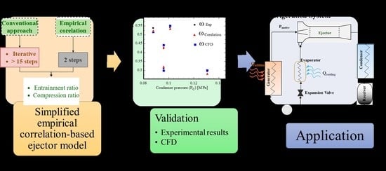
1. Introduction
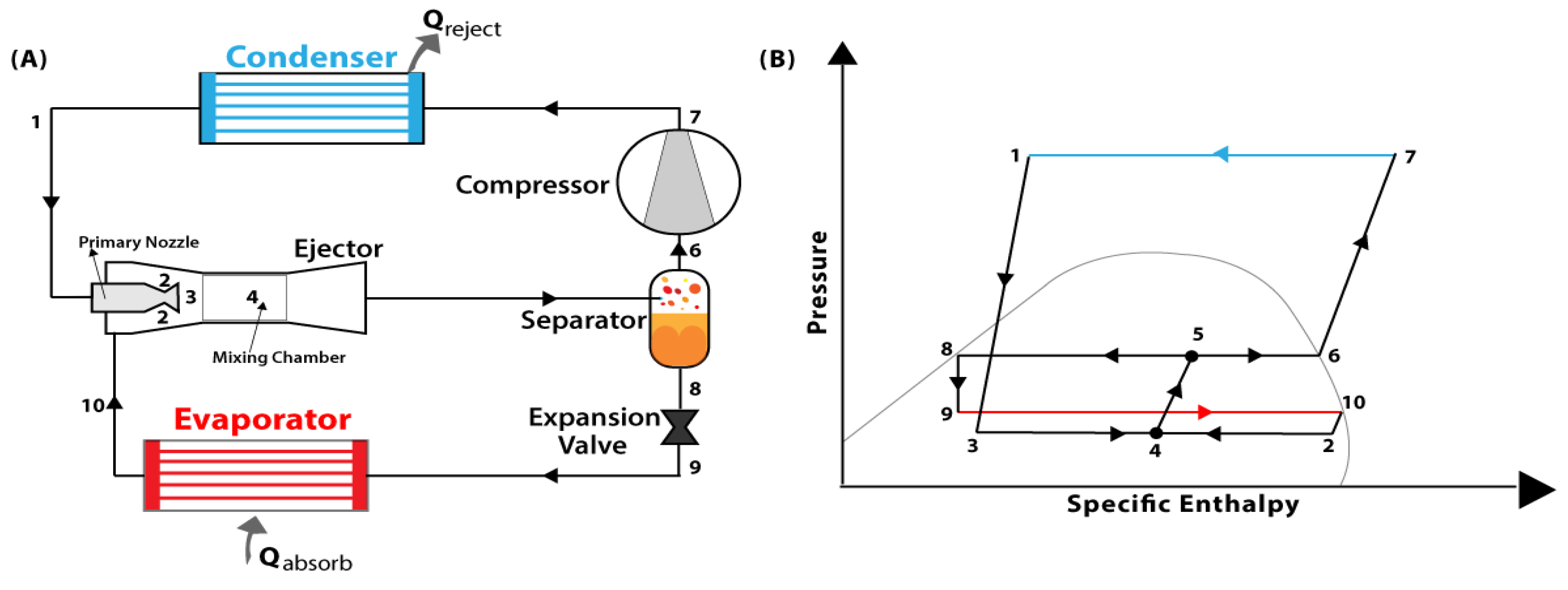
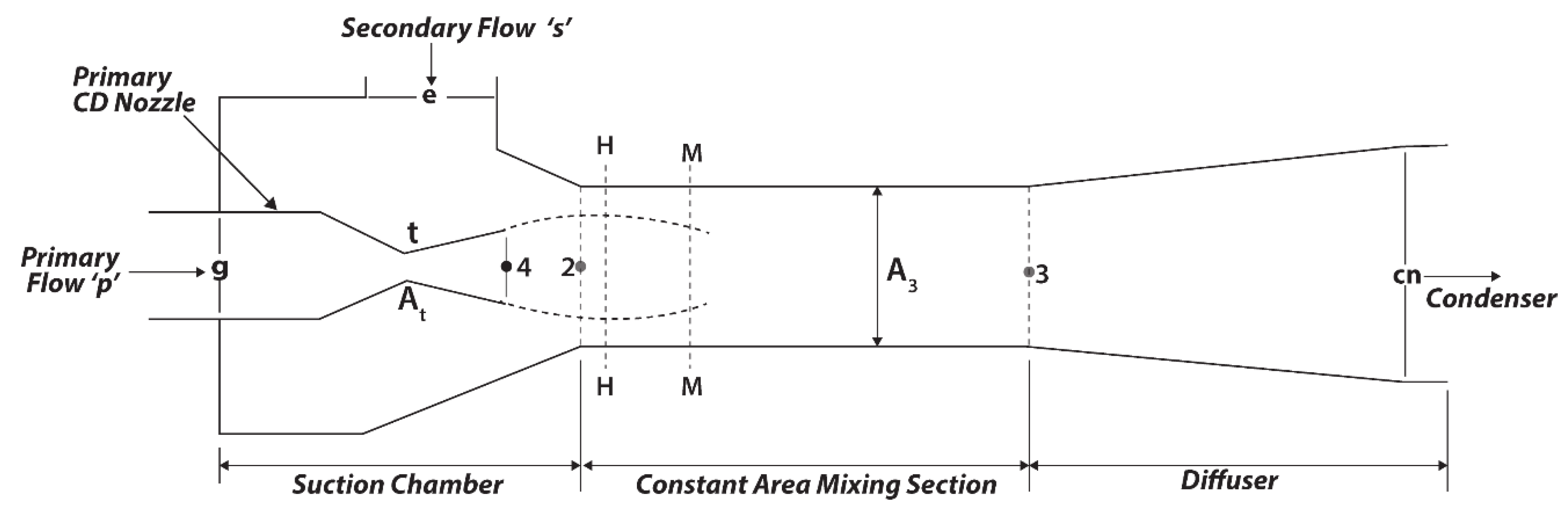
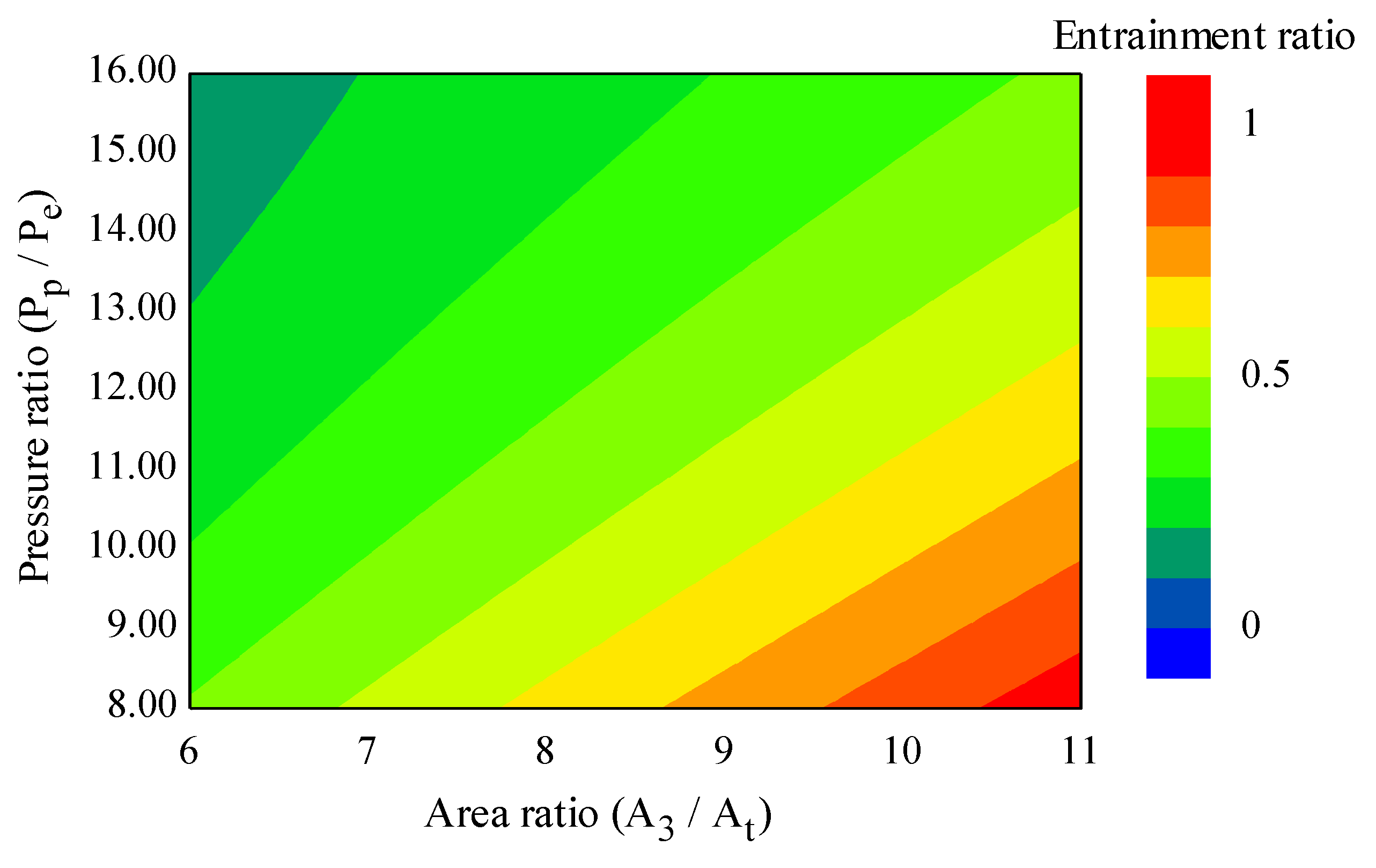
2. Ejector Description and Modeling
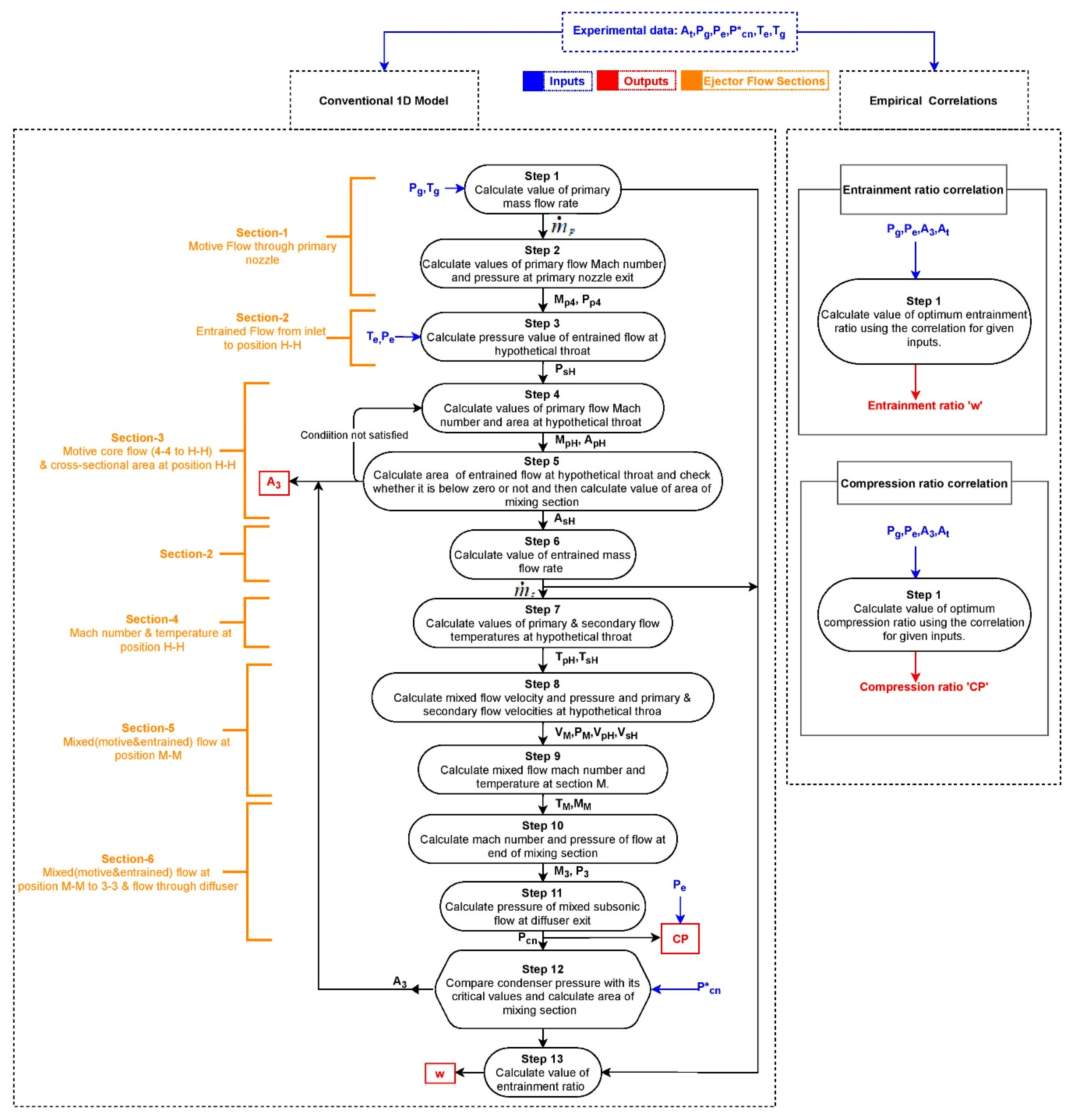
2.1. Mathematical Solution of Ejectors
- The working fluid acts as an ideal gas, having constant specific heat (Cp) and specific heat ratio (γ).
- Steady, adiabatic, and 1D flow.
- Negligible kinetic energy at secondary flow inlet, primary nozzle inlet, and diffuser exit.
- Use of isentropic relations and constant mixing chamber efficiency.
- The primary and secondary fluid flow mixes at hypothetical throat located within constant area section (Section 2–3).
- Constant pressure mixing (PpH = PsH).
- Choking of entrained flow at hypothetical throat and Mach number of MsH = 1 is assumed.
- Adiabatic ejector walls.
2.2. Mathematical Solution of Ejectors
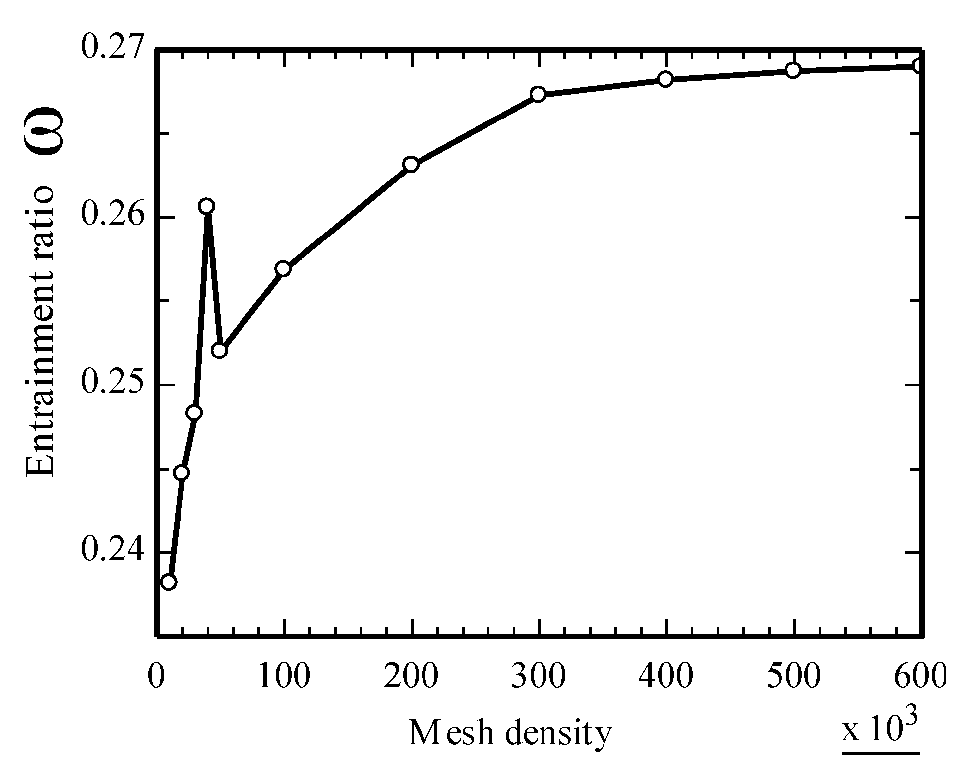
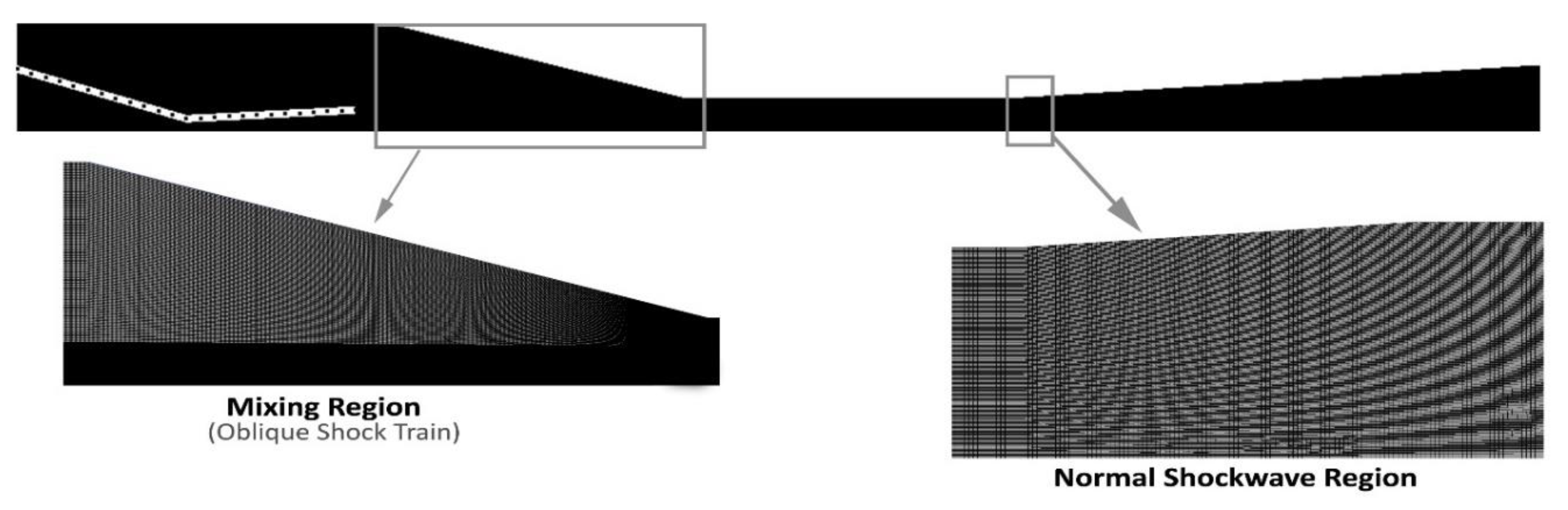
2.3. CFD Model Validation
3. Results
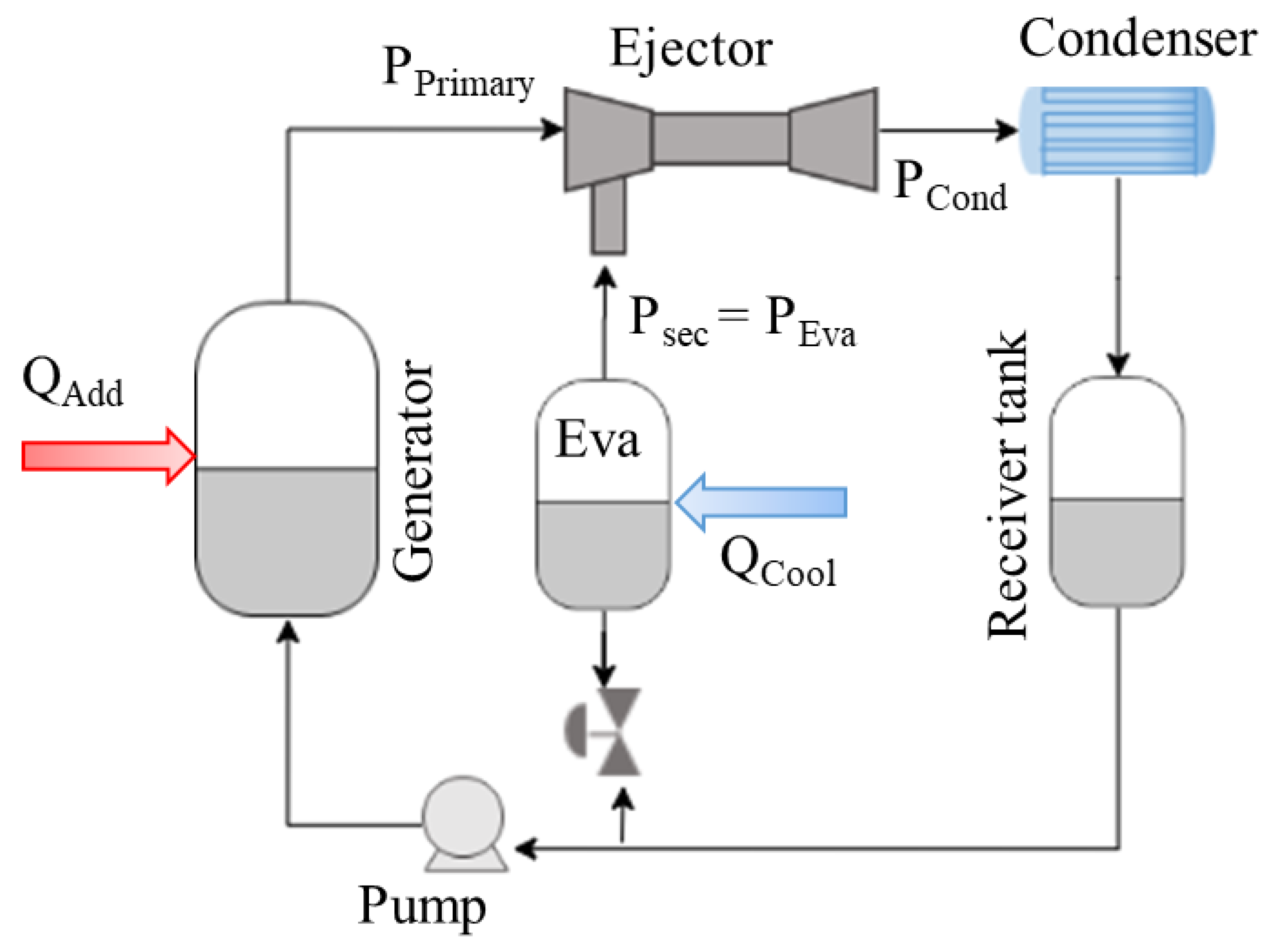
3.1. Case Study: Simple Refrigeration Machine
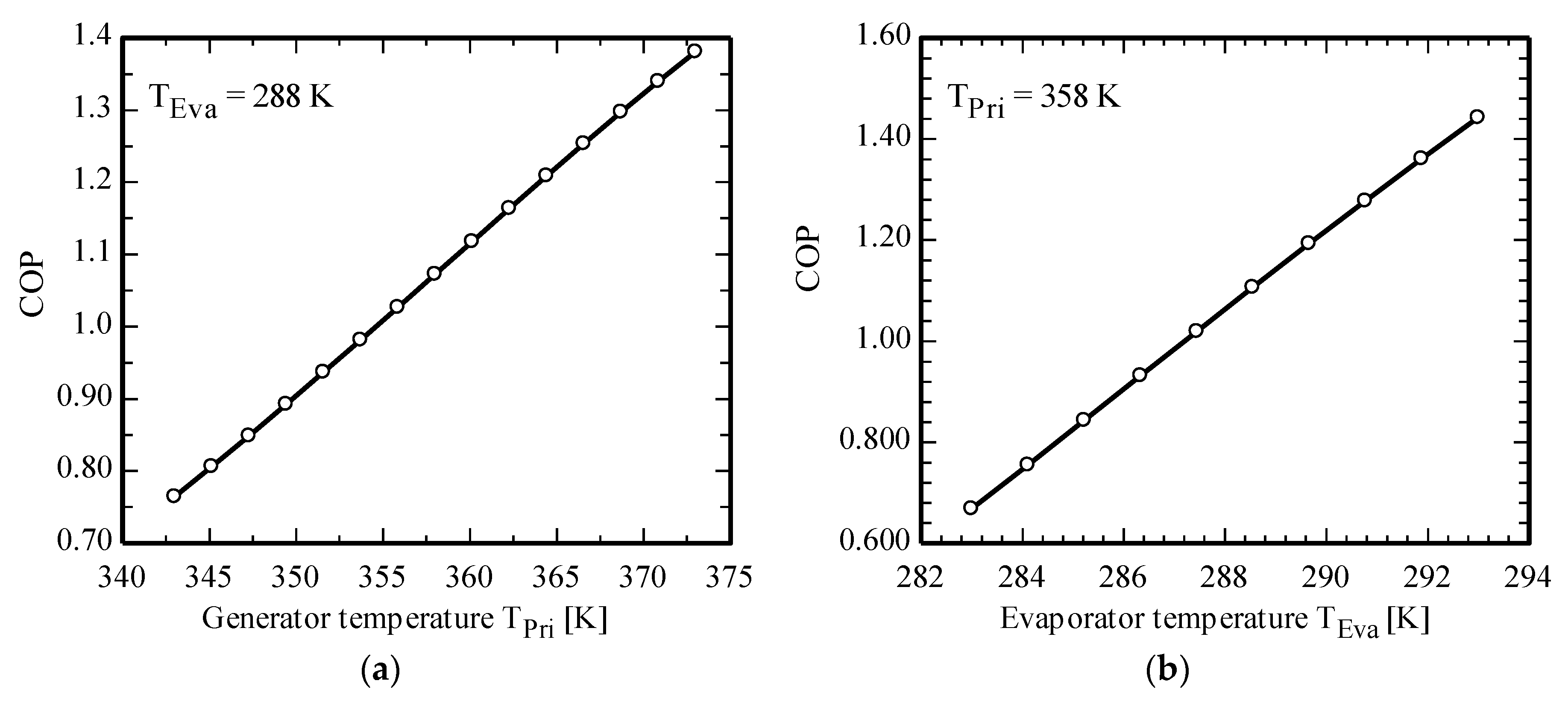
3.2. COP Variation with Generation Temperature and the Evaporation Temperature
4. Conclusions
Author Contributions
Funding
Conflicts of Interest
Nomenclature
| D | Diameter |
| A | Area, m2 |
| Cp | Fluid specific heat at constant pressure, KJ kg−1 K−1 |
| Cv | Fluid specific heat at constant volume, KJ kg−1 K−1 |
| γ | Ratio of specific heats (Cp/Cv) |
| R | Specific gas constant, KJ kg−1 K−1 |
| a | Sonic velocity, ms−1 |
| V | Fluid velocity, ms−1 |
| M | Mach number |
| m | Mass flowrate, kgs−1 |
| h | Enthalpy, KJ kg−1 |
| Pg | Fluid pressure at ejector primary nozzle inlet, MPa |
| Pe | Fluid pressure at ejector suction inlet, MPa |
| Pcn * | Ejector critical back pressure, MPa |
| T | Temperature, K |
| Tg | Fluid temperature at ejector primary nozzle inlet, K |
| Te | Fluid temperature at ejector suction inlet, MPa |
| Tcn * | Saturated vapor temperature corresponding to Pcn *, K |
| Tgs | Saturated-vapor temperature corresponding to Pg, K |
| H | Hypothetical throat position |
| ƞ | Isentropic efficiency coefficient |
| φ | Coefficient representing flow losses |
| Superscripts | |
| * | Ejector critical operation mode |
| Subscripts | |
| cn | Condenser, Ejector exit |
| e | Entrained flow suction port |
| g | Primary nozzle inlet |
| M | Mixed flow |
| t | Primary nozzle throat |
| p4 | Primary fluid at nozzle exit |
| sH | Entrained flow at hypothetical throat |
| pH | Primary flow at hypothetical throat |
| 1 | Motive nozzle throat |
| 2 | Constant area section Entrance |
| 3 | Constant area section Exit |
| 4 | Primary Nozzle Exit |
Appendix A
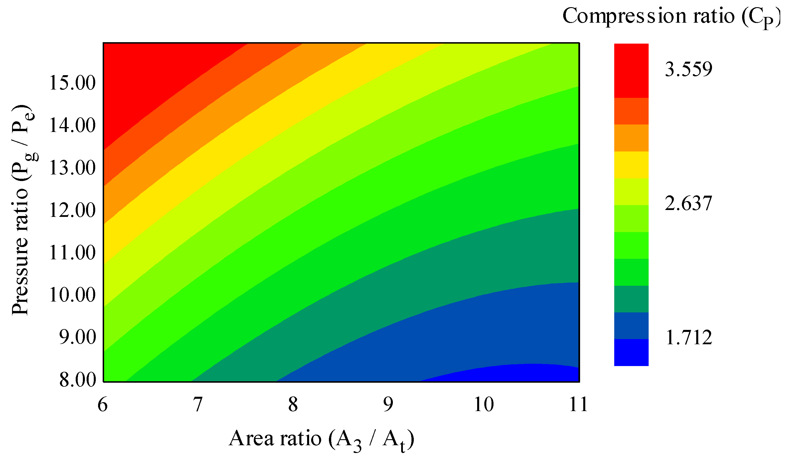
| Geometry | Area Ratio (A3/At) | Expansion Ratio (Pg/Pe) | Compression Ratio (Pc/Pe) | Entrainment Ratio (ω) |
| AA | 6.44 | 10 | 2.56 | 0.3257 |
| 6.44 | 11.62 | 2.84 | 0.288 | |
| 6.44 | 13.45 | 3.18 | 0.2246 | |
| 6.44 | 15.1 | 3.54 | 0.1859 | |
| 6.44 | 9.89 | 2.45 | 0.3398 | |
| 6.44 | 11.44 | 2.76 | 0.2946 | |
| 6.44 | 12.85 | 3.05 | 0.235 | |
| EG | 6.77 | 15.1 | 3.41 | 0.2043 |
| AB | 6.99 | 10 | 2.3 | 0.3922 |
| 6.99 | 11.62 | 2.66 | 0.3117 | |
| 6.99 | 13.45 | 3.04 | 0.2718 | |
| EC | 7.26 | 15.1 | 3.17 | 0.2273 |
| 7.26 | 12.85 | 2.74 | 0.304 | |
| AG | 7.73 | 10 | 2.26 | 0.4393 |
| 7.73 | 11.62 | 2.54 | 0.3883 | |
| 7.73 | 13.45 | 2.95 | 0.304 | |
| 7.73 | 15.1 | 3.15 | 0.2552 | |
| 7.73 | 8.51 | 1.93 | 0.6132 | |
| 7.73 | 9.89 | 2.17 | 0.479 | |
| 7.73 | 11.44 | 2.45 | 0.4034 | |
| 7.73 | 12.85 | 2.69 | 0.3503 | |
| ED | 8.25 | 15.1 | 3 | 0.2902 |
| AC | 8.29 | 10 | 2.09 | 0.4889 |
| 8.29 | 11.62 | 2.38 | 0.4241 | |
| 8.29 | 13.45 | 2.67 | 0.3488 | |
| 8.29 | 15.1 | 2.91 | 0.2814 | |
| EE | 9.17 | 15.1 | 2.71 | 0.3505 |
| 9.17 | 12.85 | 2.31 | 0.4048 | |
| AD | 9.41 | 10 | 1.91 | 0.6227 |
| 9.41 | 11.62 | 2.18 | 0.5387 | |
| 9.41 | 13.45 | 2.47 | 0.4446 | |
| 9.41 | 15.1 | 2.66 | 0.3457 | |
| 9.41 | 8.51 | 1.7 | 0.7412 | |
| 9.41 | 9.89 | 1.91 | 0.635 | |
| 9.41 | 11.44 | 2.14 | 0.5422 | |
| 9.41 | 12.85 | 2.33 | 0.4541 | |
| 9.83 | 15.1 | 2.6 | 0.3937 | |
| 9.83 | 12.85 | 2.22 | 0.4989 | |
| EH | 10.64 | 15.1 | 2.45 | 0.4377 |
References
- Li, A.; Yuen, A.C.Y.; Chen, T.B.Y.; Wang, C.; Liu, H.; Cao, R.; Yang, W.; Yeoh, G.H.; Timchenko, V. Computational study of wet steam flow to optimize steam ejector efficiency for potential fire suppression application. Appl. Sci. 2019, 9, 1486. [Google Scholar] [CrossRef]
- Nadig, R. Evacuation systems for steam surface condensers: Vacuum pumps or steam jet air ejectors? In ASME 2016 Power Conference Collocated with the ASME 2016 10th International Conference on Energy Sustainability and the ASME 2016 14th International Conference on Fuel Cell Science, Engineering and Technology; American Society of Mechanical Engineers Digital Collection: Charlotte, NC, USA, 2016. [Google Scholar]
- Pourmohammadbagher, A.; Jamshidi, E.; Ale-Ebrahim, H.; Dabir, B.; Mehrabani-Zeinabad, M. Simultaneous removal of gaseous pollutants with a novel swirl wet scrubber. Chem. Eng. Process. Process Intensif. 2011, 50, 773–779. [Google Scholar] [CrossRef]
- Liu, J.; Wang, L.; Jia, L.; Xue, H. Thermodynamic analysis of the steam ejector for desalination applications. Appl. Therm. Eng. 2019, 159, 113883. [Google Scholar] [CrossRef]
- Vincenzo, L.; Pagh, N.M.; Knudsen, K.S. Ejector design and performance evaluation for recirculation of anode gas in a micro combined heat and power systems based on solid oxide fuel cell. Appl. Therm. Eng. 2013, 54, 26–34. [Google Scholar] [CrossRef]
- Genc, O.; Timurkutluk, B.; Toros, S. Performance evaluation of ejector with different secondary flow directions and geometric properties for solid oxide fuel cell applications. J. Power Sources 2019, 421, 76–90. [Google Scholar] [CrossRef]
- Chen, J.; Jarall, S.; Havtun, H.; Palm, B. A review on versatile ejector applications in refrigeration systems. Renew. Sustain. Energy Rev. 2015, 49, 67–90. [Google Scholar] [CrossRef]
- Xia, J.; Wang, J.; Zhou, K.; Zhao, P.; Dai, Y. Thermodynamic and economic analysis and multi-objective optimization of a novel transcritical CO2 Rankine cycle with an ejector driven by low grade heat source. Energy 2018, 161, 337–351. [Google Scholar] [CrossRef]
- Chunnanond, K.; Aphornratana, S. Ejectors: Applications in refrigeration technology. Renew. Sustain. Energy Rev. 2004, 8, 129–155. [Google Scholar] [CrossRef]
- Elbel, S.; Lawrence, N. Review of recent developments in advanced ejector technology. Int. J. Refrig. 2016, 62, 1–18. [Google Scholar] [CrossRef]
- Besagni, G.; Mereu, R.; Inzoli, F. Ejector refrigeration: A comprehensive review. Renew. Sustain. Energy Rev. 2016, 53, 373–407. [Google Scholar] [CrossRef]
- Riaz, F.; Lee, P.S.; Chou, S.K. Thermal modelling and optimization of low-grade waste heat driven ejector refrigeration system incorporating a direct ejector model. Appl. Therm. Eng. 2020, 167, 114710. [Google Scholar] [CrossRef]
- Lucas, C.; Koehler, J. Experimental investigation of the COP improvement of a refrigeration cycle by use of an ejector. Int. J. Refrig. 2012, 35, 1595–1603. [Google Scholar] [CrossRef]
- Aligolzadeh, F.; Hakkaki-Fard, A. A novel methodology for designing a multi-ejector refrigeration system. Appl. Therm. Eng. 2019, 151, 26–37. [Google Scholar] [CrossRef]
- Huang, B.J.; Chang, J.M.; Wang, C.P.; Petrenko, V.A. A 1-D analysis of ejector performance. Int. J. Refrig. 1999, 22, 354–364. [Google Scholar] [CrossRef]
- Haghparast, P.; Sorin, M.V.; Nesreddine, H. Effects of component polytropic efficiencies on the dimensions of monophasic ejectors. Energy Convers. Manag. 2018, 162, 251–263. [Google Scholar] [CrossRef]
- Selvaraju, A.; Mani, A. Analysis of an ejector with environment friendly refrigerants. Appl. Therm. Eng. 2004, 24, 827–838. [Google Scholar] [CrossRef]
- Aidoun, Z.; Ameur, K.; Falsafioon, M.; Badache, M. Current Advances in Ejector Modeling, Experimentation and Applications for Refrigeration and Heat Pumps. Part 1: Single-Phase Ejectors. Inventions 2019, 4, 15. [Google Scholar] [CrossRef]
- Aidoun, Z.; Ameur, K.; Falsafioon, M.; Badache, M. Current Advances in Ejector Modeling, Experimentation and Applications for Refrigeration and Heat Pumps. Part 2: Two-Phase Ejectors. Inventions 2019, 4, 16. [Google Scholar] [CrossRef]
- Desevaux, P.; Marynowski, T.; Khan, M. CFD prediction of supersonic ejectors performance. Int. J. Turbo Jet Engines 2006, 23, 173–182. [Google Scholar] [CrossRef]
- Del Valle, J.G.; Sierra-Pallares, J.; Carrascal, P.G.; Ruiz, F.C. An experimental and computational study of the flow pattern in a refrigerant ejector. Validation of turbulence models and real-gas effects. Appl. Therm. Eng. 2015, 89, 795–811. [Google Scholar] [CrossRef]
- Han, Y.; Wang, X.; Sun, H.; Zhang, G.; Guo, L.; Tu, J. CFD simulation on the boundary layer separation in the steam ejector and its influence on the pumping performance. Energy 2019, 167, 469–483. [Google Scholar] [CrossRef]
- Elbarghthi, A.F.; Mohamed, S.; Nguyen, V.V.; Dvorak, V. CFD Based Design for Ejector Cooling System Using HFOS (1234ze (E) and 1234yf). Energies 2020, 13, 1408. [Google Scholar] [CrossRef]
- Little, A.B.; Garimella, S. A critical review linking ejector flow phenomena with component-and system-level performance. Int. J. Refrig. 2016, 70, 243–268. [Google Scholar] [CrossRef]
- Wen, C.; Rogie, B.; Kærn, M.R.; Rothuizen, E. A first study of the potential of integrating an ejector in hydrogen fuelling stations for fuelling high pressure hydrogen vehicles. Appl. Energy 2020, 260, 113958. [Google Scholar] [CrossRef]
- Zhu, Y.; Jiang, P. Experimental and numerical investigation of the effect of shock wave characteristics on the ejector performance. Int. J. Refrig. 2014, 40, 31–42. [Google Scholar] [CrossRef]
- He, S.; Li, Y.; Wang, R.Z. Progress of mathematical modeling on ejectors. Renew. Sustain. Energy Rev. 2009, 13, 1760–1780. [Google Scholar] [CrossRef]
- Croquer, S.; Poncet, S.; Aidoun, Z. Turbulence modeling of a single-phase R134a supersonic ejector. Part 1: Numerical benchmark. Int. J. Refrig. 2016, 61, 140–152. [Google Scholar] [CrossRef]
- Tashtoush, B.M.; Moh’d A, A.N.; Khasawneh, M.A. A comprehensive review of ejector design, performance, and applications. Appl. Energy 2019, 240, 138–172. [Google Scholar] [CrossRef]
- Rawlings, J.O.; Pantula, S.G.; Dickey, D.A. Applied Regression Analysis: A Research Tool; Springer Science & Business Media: Berlin/Heidelberg, Germany, 2001. [Google Scholar]
- Sinha, P. Multivariate polynomial regression in data mining: Methodology, problems and solutions. Int. J. Sci. Eng. Res. 2013, 4, 962–965. [Google Scholar]
- Honra, J.; Berana, M.S.; Danao, L.A.M.; Manuel, M.C.E. CFD Analysis of Supersonic Ejector in Ejector Refrigeration System for Air Conditioning Application. In Proceedings of the World Congress on Engineering, London, UK, 5–7 July 2017; Volume 2. [Google Scholar]
- Carrillo, J.A.E.; de La Flor, F.J.S.; Lissén, J.M.S. Single-phase ejector geometry optimisation by means of a multi-objective evolutionary algorithm and a surrogate CFD model. Energy 2018, 164, 46–64. [Google Scholar] [CrossRef]
- Pianthong, K.; Seehanam, W.; Behnia, M.; Sriveerakul, T.; Aphornratana, S. Investigation and improvement of ejector refrigeration system using computational fluid dynamics technique. Energy Convers. Manag. 2007, 48, 2556–2564. [Google Scholar] [CrossRef]
- Zhang, H.; Wang, L.; Jia, L.; Wang, X. Assessment and prediction of component efficiencies in supersonic ejector with friction losses. Appl. Therm. Eng. 2018, 129, 618–627. [Google Scholar] [CrossRef]
- Bartosiewicz, Y.; Aidoun, Z.; Desevaux, P.; Mercadier, Y. Cfd-experiments integration in the evaluation of six turbulence models for supersonic ejector modeling. Integr. CFD 2003, 1, 450. [Google Scholar]
- Hanafi, A.S.; Mostafa, G.M.; Waheed, A.; Fathy, A. 1-D mathematical modeling and CFD investigation on supersonic steam ejector in MED-TVC. Energy Procedia 2015, 75, 3239–3252. [Google Scholar] [CrossRef]
- Besagni, G.; Inzoli, F. Computational fluid-dynamics modeling of supersonic ejectors: Screening of turbulence modeling approaches. Appl. Therm. Eng. 2017, 117, 122–144. [Google Scholar] [CrossRef]
- Besagni, G.; Mereu, R.; Chiesa, P.; Inzoli, F. An Integrated Lumped Parameter-CFD approach for off-design ejector performance evaluation. Energy Convers. Manag. 2015, 105, 697–715. [Google Scholar] [CrossRef]
- Mohamed, S.; Shatilla, Y.; Zhang, T. CFD-based design and simulation of hydrocarbon ejector for cooling. Energy 2019, 167, 346–358. [Google Scholar] [CrossRef]
- Scott, D.; Aidoun, Z.; Bellache, O.; Ouzzane, M. CFD simulations of a supersonic ejector for use in refrigeration applications. In Proceedings of the International Refrigeration and Air Conditioning Conference at Purdue, Paper 927. West Lafayette, IN, USA, 14–17 July 2008. [Google Scholar]


| Ejector Geometry | ||||
|---|---|---|---|---|
| Primary Nozzle | Mixing (Constant Area) Section | |||
| Serial No. | Diameter (D3) | |||
| Serial No. | Throat Diameter (Dt) | Exit Diameter (D4) | A | 6.70 mm |
| A | 2.64 mm | 4.50 mm | B | 6.98 mm |
| C | 7.60 mm | |||
| D | 8.10 mm | |||
| E | 2.82 mm | 5.10 mm | E | 8.54 mm |
| G | 7.34 mm | |||
| H | 9.20 mm | |||
| Step | Inputs | Equations | Output | Comments |
|---|---|---|---|---|
| 1 | At choking condition, the mass flow rate through the primary nozzle follows a gas dynamic relation. | |||
| 2 | The Mach no. M4 is calculated by using the Newton–Raphson method. | |||
| 3 | Referring to the assumptions made, the Mach number of secondary flow at hypothetical throat is MeH = 1. | |||
| 4 | : an isentropic coefficient that represents flow losses as primary fluid flow from section 4-4 to section H-H. | |||
| 5 | If AsH < 0, calculate A3 by using A3 = ApH + ΔA3, otherwise return to step 4 to recalculate ApH, and again the condition is checked. | |||
| 6 | : Isentropic efficiency of entrained flow. | |||
| 7 | Value of Tg and Te can be taken from step 1 and 3, respectively. | |||
| 8 | : mixed flow friction coefficient, PM = PpH = PsH, MsH = 1, and MpH can be taken from step 4. | |||
| 9 | The first equation gives TM, which is then used to find value of αM and MM. | |||
| 10 | Flow is solved after the shock wave, and value of PM can be taken from step 8. | |||
| 11 | Flow pressure at diffuser exit is calculated. | |||
| 12 | : critical condenser pressure, and A3 must be equal to A3 in step 5, otherwise procedure starts again from step 5. | |||
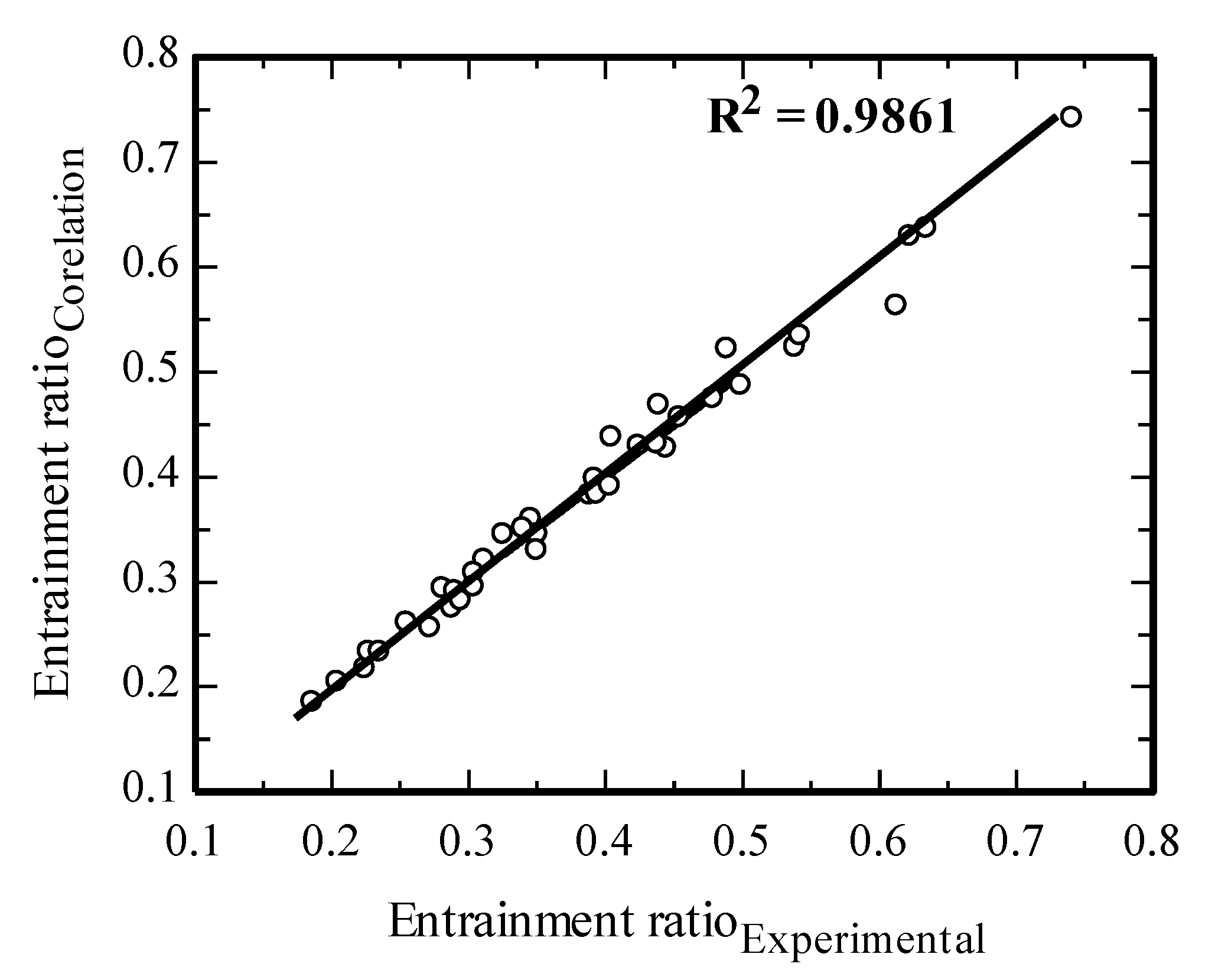
| 13 | Entrainment ratio is calculated by using ṁs and ṁp from step 6 and step 1, respectively. |
| Mesh | |
| Mesh Type | Structured |
| Number of elements | 500,000 |
| Element type | Quadratic quadrilateral |
| Boundary Conditions | |
| Primary flow inlet | Pressure inlet |
| Secondary flow inlet | Pressure inlet |
| Discharge flow outlet | Pressure outlet |
| Numerical Model Setup | |
| Solver | Pressure based |
| Turbulence model | k-ω-sst |
| Method of initialization | Hybrid |
| Fluid density | Ideal gas |
| Working fluid | R141b |
| Discretization scheme | Second order upwind |
| Convergence criteria | Residuals <10−6 |
| Parameters | Values |
|---|---|
| Refrigeration capacity (QCool) | 300 W |
| Required condensing saturation temperature (TCond,Req) | 40 °C |
| Generator saturation temperature (TPri) | 70–100 °C |
| Evaporator saturation temperature (TEva) | 10–20 °C |
| Component | Input | Output | Equations | Comment |
|---|---|---|---|---|
| Evaporator | QCool, TEva | msec | Since the saturation temperature is known, Δhfg can be calculated. | |
| Ejector | msec, A3/AT, PPri/PEva | ω, PCond, mPri | Using the developed co-relation, the ω and PCond can be calculated. If then iterate A3/At. | |
| Generator | TPri, mPri | QAdd | Since the saturation temperature is known, Δhfg can be calculated. |
Publisher’s Note: MDPI stays neutral with regard to jurisdictional claims in published maps and institutional affiliations. |
© 2020 by the authors. Licensee MDPI, Basel, Switzerland. This article is an open access article distributed under the terms and conditions of the Creative Commons Attribution (CC BY) license (http://creativecommons.org/licenses/by/4.0/).
Share and Cite
Muhammad, H.A.; Abdullah, H.M.; Rehman, Z.; Lee, B.; Baik, Y.-J.; Cho, J.; Imran, M.; Masud, M.; Saleem, M.; Butt, M.S. Numerical Modeling of Ejector and Development of Improved Methods for the Design of Ejector-Assisted Refrigeration System. Energies 2020, 13, 5835. https://doi.org/10.3390/en13215835
Muhammad HA, Abdullah HM, Rehman Z, Lee B, Baik Y-J, Cho J, Imran M, Masud M, Saleem M, Butt MS. Numerical Modeling of Ejector and Development of Improved Methods for the Design of Ejector-Assisted Refrigeration System. Energies. 2020; 13(21):5835. https://doi.org/10.3390/en13215835
Chicago/Turabian StyleMuhammad, Hafiz Ali, Hafiz Muhammad Abdullah, Zabdur Rehman, Beomjoon Lee, Young-Jin Baik, Jongjae Cho, Muhammad Imran, Manzar Masud, Mohsin Saleem, and Muhammad Shoaib Butt. 2020. "Numerical Modeling of Ejector and Development of Improved Methods for the Design of Ejector-Assisted Refrigeration System" Energies 13, no. 21: 5835. https://doi.org/10.3390/en13215835
APA StyleMuhammad, H. A., Abdullah, H. M., Rehman, Z., Lee, B., Baik, Y.-J., Cho, J., Imran, M., Masud, M., Saleem, M., & Butt, M. S. (2020). Numerical Modeling of Ejector and Development of Improved Methods for the Design of Ejector-Assisted Refrigeration System. Energies, 13(21), 5835. https://doi.org/10.3390/en13215835