Abstract
In the present numerical study, implicit large eddy simulations (LES) of non-reacting multi-components mixing processes of cryogenic nitrogen and n-dodecane fuel injections under transcritical and supercritical conditions are carried out, using a modified reacting flow solver, originally available in the open source software OpenFOAM®. To this end, the Peng-Robinson (PR) cubic equation of state (EOS) is considered and the solver is modified to account for the real-fluid thermodynamics. At high pressure conditions, the variable transport properties such as dynamic viscosity and thermal conductivity are accurately computed using the Chung transport model. To deal with the multicomponent species mixing, molar averaged homogeneous classical mixing rules are used. For the velocity-pressure coupling, a PIMPLE based compressible algorithm is employed. For both cryogenic and non-cryogenic fuel injections, qualitative and quantitative analyses are performed, and the results show significant effects of the chamber pressure on the mixing processes and entrainment rates. The capability of the proposed numerical model to handle multicomponent species mixing with real-fluid thermophysical properties is demonstrated, in both supercritical and transcritical regimes.
1. Introduction
Fuel injections in cryogenic rockets, high-pressure diesel engines, or gas-turbines, operating at transcritical and supercritical conditions, have gained a significant interest following the perspective of emission reduction and improvement of engine efficiency. In these applications, fuel injections in high-pressure and high-temperature conditions have recently been considered as a way to enhance the engine thermal efficiency and the power output, with reduced soot and NOx emissions [1]. These elevated pressure conditions translate to chambers operating at pressures and temperatures exceeding fuel critical values. This eventually creates the supercritical dense flow conditions with negligible effect of surface tension and the latent heat of vaporization displays where the turbulent jet becomes soluble [2]. The state of the injected fluid is at either transcritical or supercritical conditions, based on whether the fuel injection temperature is below or above the pseudo-boiling temperature, Tpb [3]. At subcritical conditions, the initial liquid jet, exhibiting surface tension, is broken-up through successive steps into liquid ligaments and fine atomized droplets, which then undergo evaporation and subsequent ignition. The jet disintegration behavior occurring under transcritical and supercritical conditions deviates from the subcritical conditions where the formation of liquid ligaments and droplets are replaced by turbulent gas jet mixing processes with widening of the diffusion layer of the liquid-gas interface [4,5].
At high pressure conditions, the intermolecular forces become significant in determining the real-fluid behavior [6]. Near the pseudo-boiling line (PBL), the thermophysical properties become highly nonlinear functions of temperature, pressure and species mole fraction. This prolonged “phase change” line, also identified as the “Widom line”, is the locus of thermophysical properties maxima, or minima, which separates the liquid-like from the gas-like behavior in the supercritical regime. Real-fluid behaviors are characterized by pressure-dependent thermophysical properties. In the context of fuel jets, the main resulting feature is that the flow is determined by a balance between mechanical jet breakup and miscible mixing. The controlling and dominant effect is then determined by the level of supercriticality of the flow.
Second law of thermodynamics plays a crucial role in the stability of a two-phase system at specified pressure, temperature, and compositions, with equilibrium determined by minimum Gibbs free energy [7]. At the critical point (CP) and above, the difference between vapor and liquid phases vanishes and the mixture becomes a structureless, homogeneous, and continuous single-phase supercritical flow [8]. Based on the literature, it is observed that the behavior of the fuel injection into a combustion chamber at supercritical quiescent ambient condition is quite different from the subcritical condition [9]. The nature of atomization is substantially different and it departs significantly from the classical cascade attributed to low-pressure liquid jet atomization. At high chamber pressures, detailed understanding is needed regarding jet mixing process with surrounding environment, plume growth rate, evolution and response of flow fields, time and length scales, and combustion zone behavior.
In the existing literature, the injection of cryogenic liquid propellants at various operating conditions is extensively investigated experimentally in [8,9,10] and numerically in [6,11,12,13,14,15,16]. Chehroudi et al. [10] conducted experimental studies on cryogenic liquid nitrogen at various pressure conditions, from subcritical to supercritical levels. They noted that surface instabilities promote mechanical breakup of the liquid surface under subcritical conditions, while at supercritical conditions a more diffuse behavior was observed resembling a turbulent gas jet. As far as air/fuel mixtures are concerned, Davis and Chehroudi [17] carried out experimental studies for cryogenic liquid rockets on the combustion thermo-acoustic instability under subcritical, transcritical, and supercritical pressure conditions. Falgout et al. [18] using ballistic imaging and ultrafast shadowgraphy technique studied different diesel-like pure fuels spray injected into air at different conditions, and concluded that the changes observed in the spray behavior scaled well with the estimated air/fuel mixture critical properties. Using high-speed visualization, Crua et al. [19] experimentally studied the transition of microscopic fuel droplets to supercritical fluid with diffusive mixing process, focusing on the end of injection of typical diesel sprays analyzing relatively large and slow moving droplets. Segal and Polikhov [20], with planar laser induced fluorescence, studied the jet surface stability and proved that typical subcritical correlations fail to predict trans- and super-critical regimes. All these studies, therefore, confirm the large interest in investigating transcritical and supercritical states in fuel injection processes in the context of high-pressure combustion chambers.
At the same time, to complement experimental investigations, the development of accurate models for both subcritical and supercritical multicomponent flows has been a long-lasting challenge. No single model is universally capable of addressing the extremely wide scenario of flow regimes. To simulate subcritical multi-phase multi-component flows, various numerical methods such as Lagrangian (moving particles), Eulerian (fixed grid) [21], and Lagrangian-Eulerian (fixed grid with moving particles) approaches can be used, but Eulerian approaches are the most common in many fields. Among these, diffuse interface models [22,23,24,25,26] are being developed with various levels of sophistication to account for unresolved mesoscale mixing, even if many challenges are still present regarding the validity of these closures. To investigate the details of separated flows, Eulerian interface capturing methods, such as level set (LS) [27], Volume of Fluid (VOF) [28], and Coupled Level Set and Volume of Fluid (CLSVOF) [29,30,31,32,33], have been progressively developed and improved, achieving nowadays high accuracy in mass conservation, surface tension force evaluation and phase change. However, all these models become numerically challenging and computationally expensive when large thermophysical properties variations are involved.
For trans- and super-critical environments, there is a widespread consensus that single-fluid diffuse interface models with real-fluid thermo-physics need to be used [34,35]. Unfortunately, Direct Numerical Simulations (DNS) will remain extremely challenging to long time for any real engineering [34] application. Among various studies of liquid injection in high pressure environments, recently, Zhang et al. [14] applied large eddy simulations (LES) model to study the jet cone angles and mixing layers with cryogens, but they were limited to pure species. However, in addition to single-fluid models, also two-fluid LES models coupled with real-fluid thermodynamics have been proposed and successfully applied for trans- and super-critical conditions [36,37]. Phase equilibrium could also be evaluated [7,36,37,38] to examine the phase stability and calculate local phase fractions. Zong and Yang [39] observed that, within the context of LES, the subgrid-scale (sgs) terms are dominant compared to molecular values, and numerical dissipation only serves to stabilize calculations. Therefore, the contribution of sgs transport properties (like turbulent viscosity) on top of accurate, but small, molecular real-fluid transport properties appears questionable. Interestingly, in the study of Gopal et al. [40], a two-fluid model with implicit LES assumption was successfully applied, using an interface compression method to deal with supercritical states, by making the interface term vanish above the critical pressure.
Combustion processes in engines add further complexities in the modelling of spray dynamics due to spatial and temporal multi-scales nature of liquid-gas interactions, mixing, complexity in finite rate of evaporation and reactions [41]. For example, the hot product gas entrainment into the fuel spray plays a significant role in the atomization, droplet dispersion [42], vaporization, and mixing [43]. The flame lift-off length and soot formation in diesel combustion engines are affected by the gas entrainment quantity in the initial spray evolution [44]. To evaluate this mixture formation effects, Sepret et al. [45] experimentally investigated the mass flow rate of gas entrainment into a non-vaporizing diesel spray and found that it depends on the distance from the nozzle and on the density of the ambient gas. Numerical modeling of gas entrainment effect has also been proposed by Pandal et al. [22], observing that the decrease in the nozzle diameter significantly increases the local mixing rate. Whether such observed behavior is manifested in sprays at transcritical and supercritical conditions needs to be further investigated.
In the present research work, an implicit large eddy simulation (LES) approach is developed for injections of cryogenic nitrogen and n-dodecane under trans- and super-critical operating conditions, considering accurate real-fluid thermophysical properties for multi-component mixtures. The simulation results are used to quantitatively characterize the mixing rate of a fuel injected in a high-pressure chamber to provide insights into the distinct characteristics of spray dynamics at near critical conditions.
2. Numerical Methodology
A fully-conservative form of the two-phase flow equations for a multi-component homogeneous mixture is considered. The C++ open source CFD software package OpenFOAM has been used as a base framework for the development of a modified solver and new libraries accounting for real-fluid thermophysical properties. Multi-component mixture properties are computed using Peng-Robinson (PR) equation of state (EOS) model [46]. To calculate viscosity and thermal conductivity, the empirical model for transport properties proposed by Chung et al. [47] is implemented. Details of the governing equations and of the real-fluid thermophysical properties models are described below.
2.1. Governing Equations and Solution Algorithm
The conservation equations are solved using a finite volume method (FVM) approach. For a fully conservative, homogeneous, compressible, non-reacting two-phase flow, the conservation equations for mass, momentum, energy, and species, within the single-fluid formulation, are given below.
where is the mixture density, is the velocity vector, is the pressure, is the viscous stress tensor, is the total specific enthalpy, is the heat flux, is the mass fraction of species i, and the species diffusion flux of species, i. Viscous stresses are closed with the compressible Newtonian fluid model. Heat flux is closed with the classical Fourier’s law, neglecting the additional contribution associated with the diffusion of species with different enthalpies. Mass diffusion fluxes are closed with the Fick’s law. Molecular thermophysical properties are evaluated using accurate real-fluid models and correlations, as detailed in the next sections. Using very fine grid in two-dimensional setups, implicit LES are conducted, therefore no additional modeled viscosity is added to the flow.
This mathematical framework considers local thermodynamic equilibrium. The velocity-pressure coupling is handled using an extended PIMPLE algorithm and a modified pressure equation [46,48] to ensure a tight coupling with momentum and thermodynamic state. To discretize the above equations, second order accurate Gauss limited-linear scheme is used for convective terms, second order accurate central differencing scheme is considered for diffusion terms, and first order accurate Euler scheme is used for the transient term. Temporal advancement is controlled by a convective Courant number below 0.5 and an acoustic Courant number below 10. The former guarantees efficiency and stability of the solution algorithm, while the latter allows to avoid unnecessary constraints related to capturing non-essential wave propagation effects in the context of spray simulations in a hot open-chamber.
2.2. Real-Fluid EOS
In the vicinity of the fluid critical point, modeling the thermodynamic state based on the ideal gas law becomes inappropriate due to the non-linear effects of intermolecular repulsive forces observed as pressure, density, composition and temperature vary. Detailed description of various EOS models are found, for example, in Poling et al. [49]. For numerical efficiency reasons, a simple EOS should be preferred, provided that it still preserves the main non-linear relationships among the thermophysical variables [50].
In the existing numerical literatures, two-parameter based cubic EOS are widely used for wide ranges of fuel injections and mixing conditions, such as Redlich-Kwong (RK), Soave-Redlich-Kwong (SRK), and Peng-Robinson (PR) models. This is mainly due to simplicity, robustness, computational efficiency, and readily available mixing rules [3]. In the present study, the two-parameter based cubic Peng-Robinson equation of state (PR-EOS) has been chosen, because it accurately computes the real-fluid thermodynamic states particularly at transcritical and supercritical conditions [51]. The compressibility factor, , is the non-dimensional parameter which quantifies the deviation from the ideal gas () behavior as,
The cubic PR-EOS equation is written as
where, p is the pressure, v is the molar specific volume, T is the temperature, x is the species mole fraction vector, and R is the universal gas constant. Coefficients a and b are model constants dependent on mixture composition, which account for the effects of intermolecular attractive forces and volume displacement, respectively. The parameter α is a function of both reduced temperature Tr = T/Tc and acentric factor ω, where the subscript ‘c’ indicates the critical condition.
For a multicomponent mixture of species, mixing and combining rules are used to extend the use of equations of state developed for pure fluids to mixtures. Typically used mixing rules for cubic EOS are the van der Waals one-fluid mixing rules, which involve binary interaction parameter between each two components, i and j [7], and directly combine the EOS parameters of pure fluids to obtain satisfactory parameters for the mixture. However, quite often, using the corresponding state principle, the mixture behavior can be described by combining critical properties of the pure species to obtain pseudocritical properties, like temperature, pressure, and molar volume applicable to the equivalent mixture. This is to say that, using the linear blend Kay’s rule, the pseudo-critical parameters can be evaluated based on molar weighted averages, as
and the mixture pseudo-critical pressure is computed as
where subscript m indicates the mixture. Then, the mixture coefficients of the EOS are computed as follows
where, the parameter is computed using an acentric factor, as
In OpenFOAM this mixing rule was originally implemented based on mass fraction , which is conceptually wrong, therefore in our work it has been corrected using molar fractions , as shown above. It is worth noticing that pseudo-critical values given by Equation (7) are merely instrumental to obtain correct densities for the mixture. The actual mixture critical temperature and pressure vary in a non-linear way with compositions. The critical temperature of the mixture generally lies between the individual pure component critical temperature values, while the mixture critical pressure may be significantly above the critical pressure values of the pure fluids.
The real-fluid caloric properties not only depend on temperature and composition, but also depend on the pressure. A real-fluid thermodynamic property, is determined as the sum of the ideal gas property and the dense fluid corrections [3,46], as
These departure functions are derived analytically from the PR EOS [3,46]. For example, the real-fluid enthalpy, , and the specific heat, , can be expressed as
where, subscript ‘0’ indicates the ideal state in the limit of very low pressure. In the above equations, the first term on the right-hand side is the ideal gas contribution depending only on temperature and species composition vector and it is obtained using standard 9-coeficients NASA polynomials [52]. While the second term on the right-hand side (known as departure functions) depends also on the pressure . The departure functions formulation can be conveniently expressed also as a function of the compressibility factor, Z, but it is not reported here for the sake of brevity [49].
2.3. Real-Fluid Chung Transport Model
The real-fluid behavior of the transport property for high pressure conditions is evaluated starting from the Chapman-Enskog theory (CET) for dilute gas viscosity at the zero density limit and corresponding state theory (CST) [53]. The dynamic viscosities of transcritical and supercritical fluids at high pressure are then calculated using the correction model proposed by Chung et al. [47].
The Chung viscosity model is based on the dilute gas formulation corrected by a multiplicative factor and by an additional additive term , both accounting for the high-pressure effects. Validations of the applicability and accuracy of this transport model in the CFD modeling framework are found in [12,53].
The dynamic viscosity is computed as follows
where is the critical volume of the mixture in cm3/mol, is the mixture density and is an empirical correlation for the reduced collision integral. The constants are linear functions of the acentric factor , the reduced dipole moment , and the association factor . The factor represents the empirical model function of the acentric factor, and it accounts for the shape and polarity of the molecules. A detailed discussion of the remaining coefficients is found in Chung et al. [47]. Similar molar weighted averages based mixing rules as aforementioned for the equation of state are applied to compute the mixture equivalent parameters, denoted with the subscript ‘m’.
This model takes care of the transition across trans-critical regimes. When the operating pressure is above the critical value, the dynamic viscosity shows a gas like behavior when the temperature is higher than the critical temperature, and it shows liquid like levels when the temperature falls below the critical value.
Similar to behavior of the dynamic viscosity, the thermal conductivity, for a high-pressure real-fluid is also well predicted using Chung et al. [47] model. The thermal conductivity is formulated as the sum of two contributions as
where the various terms follow an analogy with those of the viscosity formulation. More details on the formulation and coefficients can be found in the original work of Chung et al. [47]. The same type of mixing rules is then applied to compute the mixture parameters, needed for the calculation of the mixture thermal conductivity.
2.4. Model Implementation Remarks and Property Verifications
In each step of the PIMPLE loop, thermo-physical properties need to be updated or retrieved from the knowledge of the most recent mixture state. Specific attention has been paid to develop efficient and robust methods for updating density and temperature.
Density is evaluated through the PR-EOS described above, by computing the roots of the cubic equation of state in terms of compressibility factor , given , , and . When the temperature is below the critical value, two possible real roots are found, thus, a stability test based on the Gibbs free energy determines what root corresponds to a stable mixture while the other root, corresponding to a metastable state, is discarded. This condition is equivalent to say that if the pressure is above the saturation value the liquid-like density is chosen, while if the pressure is below the saturation level the gas-like is selected.
Retrieving temperature after the species and the energy equations are solved is also delicate. A stabilizing version of the Newton’s method is used for this task. The present approach determines the so-called “frozen temperature” [5,7,16] which, in other words, does not account for splitting into liquid and gas phase, should this be the stable state from a thermodynamic standpoint.
The verification of the implemented models has been conducted on multiple species and thermodynamic conditions. Figure 1 and Figure 2 show examples of the verification step, displaying density, specific heat, viscosity, and conductivity at different pressure levels, for different fluids, in a range spanning from subcritical to supercritical states.
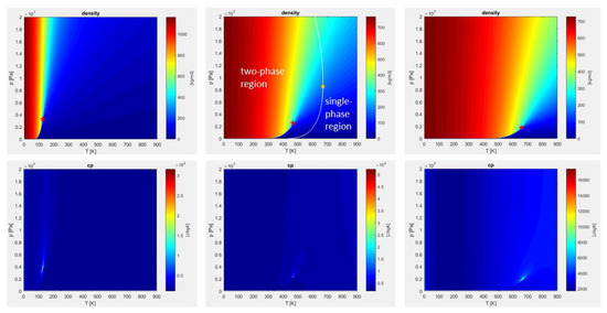
Figure 1.
Pressure-temperature plots of density and specific heat at constant pressure, for pure nitrogen (left), nitrogen/n-dodecane mixture—50% by volume (middle), pure n-dodecane (right), calculated with Peng-Robinson equation of state (PR-EOS). Red stars identify the pure and pseudo-fluid critical points. Yellow star identifies the real mixture critical point, evaluated by means of the NIST database [54].
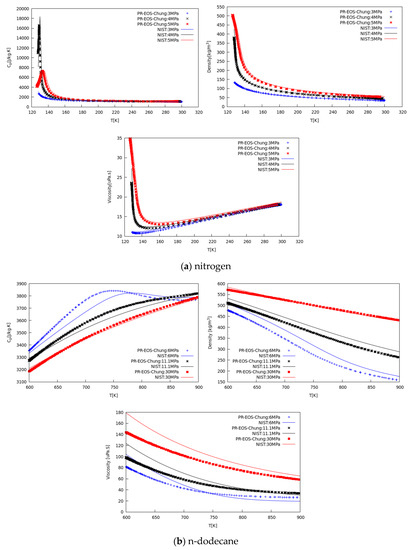
Figure 2.
Verification of CFD results (scatter points) against NIST data (line) vs. temperature for specific heat at constant pressure, density, and dynamic viscosity of (a) nitrogen at 3, 4, and 5 MPa, and (b) n-dodecane at 6, 11.1, and 30 MPa.
Figure 1 displays p-T state diagrams for nitrogen, nitrogen/n-dodecane blend, and n-dodecane. In the supercritical top-right quadrant, the density varies monotonically, while the specific heat shows very high levels in a narrow region. Following the specific heat maxima, the pseudo-boiling line (Widom line) is visualized. Red stars on the density plots mark the pure and pseudo-fluid critical points. In the mixture case, the actual critical point is marked by a yellow star, evaluated by means of the NIST database [54]. The white line superimposed on the mixture density plot is the locus of the real critical points, and separates the single-phase region from the two-phase region. It is worth noticing that properties obtained by the PR-EOS are not sufficient to identify the two regions, and additional fluid phase equilibria calculations for stability and flashing would be needed [7,23,36], which are outside the scope of this work.
Figure 2a shows the comparison between calculated properties and NIST database values for nitrogen, in the temperature range from 120 K to 300 K, at three different pressures covering from sub- to supercritical conditions. Scattered CFD data agree well with experimental data. Specific heat peaks denoting the pseudo-boiling (PB) location agree well in terms of amplitude and location. Minor discrepancies arise on the liquid density side because on the known PR behavior in this region.
Viscosity and thermal conductivity agree satisfactorily well with data suggesting the Chung model [47] is adequate for engineering CFD calculation of dense fluid mixing. In addition, Figure 2b shows the same type of comparison for n-dodecane, in the temperature range between 600 K to 900 K, for three pressure levels, from 6 MPa to 30 MPa. Similarly, the predicted properties agree satisfactorily well with NIST data [54], within the deviation range known for these correlations [47], confirming the suitability for CFD modeling of real-fluid mixing processes.
3. Results and Discussion
The turbulent jet mixing processes regarding cryogenic liquid nitrogen (L-N2) and n-dodecane injected into a quiescent gaseous nitrogen (G-N2) environment are examined, under transcritical and supercritical conditions, for various chamber pressures and injection temperatures. For an engine, a higher efficiency is obtained at higher chamber pressures. This trend has motivated many researchers to investigate higher operating pressure conditions of the combustion chamber, as the thermal efficiency and power output in rockets, gas turbines or diesel engines is shown to increase. The injected fluid at sub/trans critical temperature into supercritical condition of the chamber typically heats up beyond its critical temperature as it mixes with the surrounding hot gas before it burns inside the combustion chamber and this process is referred to as “transcritical”. The liquid rocket engines operate at conditions above the thermodynamic critical point of the injected propellants. For example, the combustion chamber pressure with the L-H2/L-O2 in Vulcain engine in the Ariane-5 can reach up to 11.5 MPa, Space Shuttle main engine was able to reach up to a maximum of 22.3 MPa [9] or more recent Merlin engines operate at 9.7 MPa.
The critical parameters such as temperature, pressure, volume, and acentric factor for nitrogen (N2) and n-dodecane (C12H26) used as working fluids in the present numerical study are tabulated in Table 1. In this numerical study, the injection of a single-component mixture, L-N2/G-N2 and a binary (multicomponent) mixture, C12H26/N2 are considered. In the case of cryogenic nitrogen into nitrogen, two species with identical properties are considered in the simulation, in order to track the injected species separately from the ambient one.

Table 1.
Critical condition parameters for pure species [46].
Following the many examples in the literature [2,13,14], to limit the computational resources needed for this type of simulations with complex thermo-physics, a 2D rectangular computational domain is used. Boundaries are treated with a pressure outlet condition on the top, bottom and right-side boundary, and no-slip and isothermal condition on the left side boundary adjacent to jet inlet. A uniform velocity and a constant injection temperature are used for the injection of the fuel. Details of computational domain with boundary conditions are shown in Figure 3.
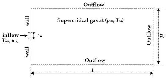
Figure 3.
Two-dimensional computational domain with boundary conditions.
In the present numerical study, both qualitative and quantitative analyses are carried out. Qualitative analyses are presented discussing several contour plots of scalar fields for the various conditions. As for the quantitative analyses, the time-averaged value of density, temperature, and velocity along axial and transverse directions are evaluated. The mean averaged quantity of any variable is reported in a non-dimensional form with respect to injected fuel conditions as
Additionally, the overall mixture (fuel + nitrogen) mass flow rate across the transverse direction is evaluated to study ambient gas entrainment in a quantitative manner. As a matter of fact, gas entrainment is an indicator of mixing. The higher the entrained gas into the jet, the higher the mixing rate. Pandal et al. [22] proposed the use of a radially integrated entrainment coefficient as a function of the axial distance from the nozzle exit. Here, equivalently, a non-dimensional normalized mass flow rate is evaluated to analyze the mixing characteristics for the various injection temperatures and chamber pressures. Along the axial direction of the chamber, the mass flow rate, , is integrated over a transverse cross-section as
where, is the spanwise dimension assumed to be 1 m, as for the 2D assumption. Using uniform inlet conditions, the injected mass flow rate at the orifice outlet is computed as
where . The non-dimensional form of the normalized mass flow rate along the chamber axial distance is obtained as
Non-dimensional quantities are used to allow the comparison of very different experiments, like the injection of cryogenic nitrogen of Mayer et al. [55] and the injection of n-dodecane, a typical diesel fuel surrogate. Detailed study of these simulations at various parameters of injection temperatures and chamber pressure conditions are below.
3.1. Validation on Cryogenic Nitrogen Jet Data
To evaluate our present numerical and physical models for the supercritical mixing processes, a comparison with experimental data of Mayer et al. [55] is considered. In real cryogenic liquid rocket engines, cryogenic liquid nitrogen (L-N2) is not used as a propellant, but due to its easy handling in experimental measurements, it is widely used as a working fluid to investigate the turbulent jet mixing characteristics of the cryogenic liquid propellants along with a high-pressure gaseous nitrogen (G-N2) as chamber quiescent environment [8,37,55]. In this study, simulation characteristics similar to Mayer’s experimental near-critical “case-3” and supercritical “case-4” are adopted where the cold cryogenic L-N2 jet is ejected from a circular nozzle of diameter d = 2.2 mm with constant injection temperature and uniform velocity into a chamber with supercritical conditions filled with a quiescent G-N2 at pressure pch = 4 MPa and temperature Tch = 298 K, respectively. The summary of these working parameters is tabulated in Table 2. Underlined conditions are referred to as the baseline conditions for the parametric study.
Table 2.
Working parameters of the cryogenic nitrogen injection case, from Mayer et al. [55].
Figure 4a reports the centerline non-dimensional time-averaged density profiles along the axial distance x/d for the validation case-3, i.e., L-N2 injected at transcritical condition of Tinj = 126.9 K ( = 439.8 kg/m3) and uinj = 4.9 m/s into G-N2 chamber at pch = 4 MPa and Tch = 298 K, compared with the experimental data (measured data extracted, = 425.5 kg/m3) of Mayer et al. [55]. The result shows the presence of an intact core region in the initial jet up to the axial length x/d ≤ 8.5. The numerical density ratio is nearly uniform and slightly over-predicted with respect to the experimental data. This can depend not only on the PR EOS inaccuracies, but also on the experimental uncertainties as documented in the original reference [55]. Moving along the jet axis, when mechanical instabilities reach the jet centerline, the dense core disappears, and the centerline density profile starts to decline. However, in the transition to fully developed turbulent jet flow region at x/d > 8.5, the numerical density profile shows a trend similar to Mayer et al. experiments [8,55] for the test case-3. Figure 4b indicates the centerline non-dimensional time-averaged density profiles along the axial distance x/d for the validation case-4, i.e., L-N2 injected at supercritical condition of Tinj = 131 K and uinj = 5.4 m/s into G-N2 chamber at pch = 4 MPa and Tch = 298 K, compared with the experimental data of Mayer et al. [55]. The result shows again that the trend is similar to experimental data, but with slight underestimation in the non-dimensional centerline density for x/d > 10. In this supercritical case-4, however, experimental density data drops after a short distance from the nozzle (from x/d > 2) and the simulation correspondingly predicts a short intact core length up to about x/d = 5, less than the transcritical case-3.
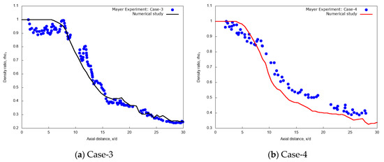
Figure 4.
Centerline time-averaged non-dimensional density ratio profile along the axial distance obtained from the present numerical study of injection of cryogenic L-N2 into supercritical chamber at pch = 4 MPa and Tch = 298 K (a) Case-3: at Tinj = 126.9 K, uinj = 4.9 m/s and (b) Case-4: at Tinj = 131 K, uinj = 5.4 m/s with uniform grid resolution per jet diameter, d/64 compared with experimental test case-3 and case-4 of Mayer et al. [55].
Acknowledging that these comparisons are not a strict validation, because of the two-dimensional setup and the absence of in-nozzle turbulence, the analysis still constitutes a positive assessment of the simulation method. Hence, the present physical models are further used to simulate injection of the cryogenic L-N2 conditions at different injection temperatures and chamber pressure conditions.
3.2. Simulations of Cryogenic L-N2 Injections into G-N2
In this subsection, the effects of various injection temperatures and chamber pressures conditions are discussed for the two-dimensional simulations of cryogenic L-N2 injection under transcritical and supercritical conditions. The entire set of injection temperatures and ambient pressures tabulated in Table 2 is considered. As before, the rectangular domain is discretized using a uniform grid size with Δx = Δy = d/64 = 0.034375 mm, resulting into a total number of 5.12 million cells. The flow dependent time step Δt is such that a maximum convective CFL equal to 0.2 is maintained. The chamber is set at room temperature Tch = 298 K. At the jet inlet, a uniform flat velocity profile with uinj = 4.9 m/s is imposed.
A first analysis concerns the variation of the injected fluid temperatures, at 4 MPa, by exploring Tinj = 126.9 K, corresponding to the N2 critical temperature, Tinj = 128.5 K, slightly below the pseudo-boiling value at the 4 MPa, and lastly Tinj = 131 K which is at supercritical.
A second analysis concerns the effect of varying chamber pressure, pch, from 4 to 6 MPa, both above the nitrogen critical pressure, at fixed injected fluid temperature Tinj = 126.9 K. These parametric studies are presented in the following subsections.
3.2.1. Effect of Injection Temperature
Here, the simulation results for the various injection temperatures aforementioned with fixed chamber conditions are discussed. Figure 5 shows instantaneous contour plots of temperature, density, pressure, dynamic viscosity, specific heat at constant pressure and velocity for the various injection temperatures Tinj, of 126.9 K (column-1), 128.5 K (column-2), and 131 K (column-3), respectively. The time shown is t = 60 ms, corresponding to about 2.5 flow-through times (FTT) of the entire domain length. These qualitatively results indicate that an increase of the injection temperature from trans to supercritical conditions leads to improved mixing processes. The velocity gradients at the jet surface generate vortex rollups and which finally break up into ligament shaped structures, similar to other numerical studies [13]. In the supercritical case (at Tinj = 131 K), no small structures are formed, while at the lower temperature (Tinj = 126.9 K) tiny structures are visible. Kelvin-Helmholtz (K-H) instabilities can be observed in a shear layer, but with different scales. As the injected fluid temperature increases, the jet is more quickly heated up to a gas-like supercritical state and mixing appears more diffusive in nature.

Figure 5.
Instantaneous contour plots obtained from simulations of cryogenic L-N2 injected at 4.9 m/s into G-N2 at supercritical chamber conditions, 4 MPa and 298 K, for various injection temperatures: first column 126.9 K, second column 128.5 K, third column 131 K. Rows, from top to bottom, show instantaneous fields of temperature T [K], density ], pressure p [Pa], dynamic viscosity ], specific heat at constant pressure cp [J/(kg K)], and velocity u [m/s].
Quantitative evaluations of the jet injection temperature effects on cryogenic L-N2 injection are considered through the centerline non-dimensional profiles of density, temperature, velocity and through the calculation of the normalized mass flow rate across the transverse direction at varying axial distance. Results are shown in Figure 6a–d, respectively. In the initial laminar jets, up to axial distance x/d ≤ 5, any noticeable effect is observed on the density, velocity, and temperature ratios that follows the variation of injected fluid temperature. Similar behavior is even kept for further axial distance up to x/d = 7 for the two lowest injection temperatures, which are, to recall, lower than the pseudo-boiling temperature. The transition region between laminar to turbulent situated at the axial distance x/d ≤ 15 shows slight deviations at various injections temperature with axial distance. Along the axial length of the chamber, as the centerline jet temperature increases the density ratio decreases, so does the corresponding velocity profile with slight fluctuations.
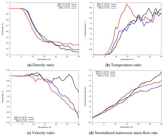
Figure 6.
Centerline axial profiles of non-dimensional density, temperature, velocity and normalized transverse mass flow rate for different injection temperatures: 126.9 K, 128.5 K, and 131 K. Simulations of cryogenic L-N2 injected at 4.9 m/s into G-N2 at 4 MPa and 298 K.
However, for the mixing rate index, or normalized transverse mass flow rate shown in Figure 6d, it is observed that the mass flow rate becomes dependent on the jet axial distance for different injection temperatures. This mass flow rate vs. axial distance diagram shows that the rate of mixing varies non-linearly in the ‘near field’ of the fuel spray. The ‘near field’ is the spray development zone where the momentum exchange between the liquid-like ligaments and the gas occurs, and which mainly contributes to the gas entrainment and the equilibrium between phases. The surrounding dense gas interact more with the liquid ‘droplets’ without apparent effect of the saturation. The rate of mixing is dominated by the density effect and the entrainment velocity of the gas is also affected by the increase in the density. When cryogenic fuel is injected at transcritical temperature, the jet temperature increases, leading to the decrease of the density profile along the axial direction. This is mainly due to the increase in the sensible heat transfer between the injected cryogenic L-N2 and the G-N2 environment.
Figure 7 shows the predicted non-dimensional radial profiles of density, temperature and velocity ratios for various injection temperatures at the axial distance x/d = 20. These results show a broader core region in terms of density and temperature for the highest jet temperature, Tinj = 131 K, which is higher than the nitrogen pseudo-boiling temperature, so fully supercritical. Furthermore, the velocity profiles do not show any significant variation in the jet core width, but it slightly reduces at the jet center for the higher degrees of supercriticality.
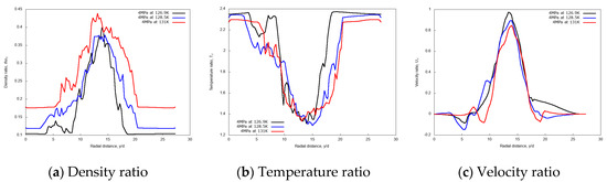
Figure 7.
Radial profiles of non-dimensional density, temperature, and velocity ratios at fixed axial distance x/d = 20, for different injection temperatures: 126.9 K, 128.5 K, and 131 K. Simulations of cryogenic L-N2 injected at 4.9 m/s into G-N2 at 4 MPa and 298 K.
3.2.2. Effects of Chamber Pressure
It is interesting now to discuss the effect of different chamber pressures on the cryogenic nitrogen injections process. Two supercritical pressures, pch levels, 4 MPa and 6 MPa, are examined, while the remaining simulation parameters are maintained constant, as specified in Table 2. Figure 8 shows the instantaneous contour plots of temperature, density, pressure, viscosity, specific heat at constant pressure and velocity obtained from the aforementioned simulations, at time t = 60 ms, corresponding, as before, to 2.5 flow-through times (FTT) of the domain length. These results show that the increase in the chamber pressure from 4 MPa to 6 MPa leads to the transition of jet behaviors from the formation of liquid-like structure to gas-like phenomena, even though the injected cryogenic nitrogen temperature is transcritical, as 126.9 K is below the corresponding PB values. For example, the density field is clearly more diffuse at high pressure than at low pressure. More quantitative analyses are needed to assess the differences, and this is addressed in the following.
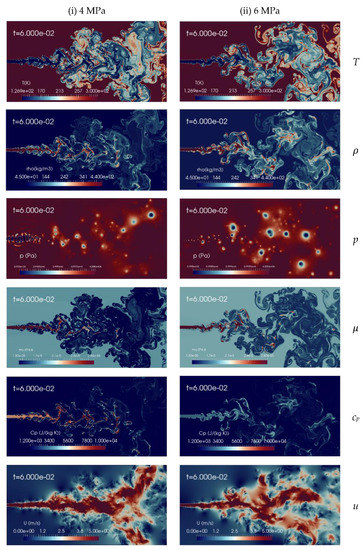
Figure 8.
Instantaneous contour plots obtained from simulations of cryogenic L-N2 injected at 126.9 K and 4.9 m/s into G-N2 at 298 K, for two different chamber pressures: first column 4 MPa, second column 6 MPa. Rows, from top to bottom, show instantaneous fields of temperature T [K], density ], pressure p [Pa], dynamic viscosity ], specific heat at constant pressure cp [J/(kg K)] and velocity u [m/s].
The centerline non-dimensional profiles of density, temperature, and velocity and the normalized transverse mass flow rate are shown in Figure 9a–d, respectively, for the two different chamber pressures. These results indicate that, due to the initial laminar jet flow conditions, the non-dimensional profiles are independent of the chamber pressure up to x/d ≤ 8.5, as the liquid-like core is still not broken-up. In the fully developed turbulent jet region, at axial distance x/d > 13, the increase of the supercritical chamber pressure leads to noticeable effects, which translate to an increase in the values of non-dimensional density, temperature and transverse mass flow rate along the axial length. The slope of the mixing rate index from the ‘near field’ to the ‘far-field’ changes for the higher pressure. This means that for the 6 MPa chamber pressure case, the turbulent jet mixing process is noticeably enhanced, compared to the 4 MPa condition.
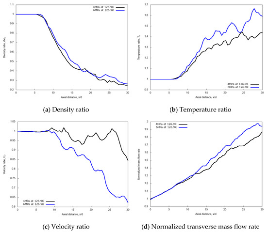
Figure 9.
Centerline axial profiles of non-dimensional density, temperature, velocity, and normalized transverse mass flow rate for different chamber pressures: 4 MPa and 6 MPa. Simulations of cryogenic L-N2 injected at 126.9 K and 4.9 m/s into G-N2 at 298 K.
Figure 10 shows the radial variations of non-dimensional density, temperature, and velocity profiles for the two different chamber pressures, at the axial distance x/d = 20. The density profile for the 6 MPa chamber pressure shows a broader core region, meaning a higher spray “cone” angle compared to the 4 MPa case. This result is in line with the findings of Zhang et al. [14], and with general expectations. A higher gas density induces higher momentum exchange and consequently more lateral diffusion. The velocity profile is less influenced by the pressure conditions except at the jet center.
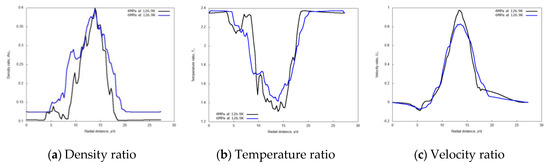
Figure 10.
Radial profiles of non-dimensional density, temperature, and velocity at fixed axial distance x/d = 20, for different chamber pressures: 4 MPa and 6 MPa. Simulations of cryogenic L-N2 injected at 126.9 K and 4.9 m/s into G-N2 at 298 K.
3.2.3. Discussion
The effect of the mixing rate at supercritical conditions is quantitatively demonstrated though the entrainment parameter. The effect of the chamber gas density is probed through the variation of the pressure at constant temperature. A denser chamber induces more mixing, on a mass-based assessment, as indicated by the normalized transverse mass flow rate curves. A broader jet is also observed under the same chamber density increase. On the contrary, little effect is observed about the injection temperature, on a normalized mass-based evaluation. The inlet temperature has been varied in a range which translate to an inlet density change close to a 2-to-1 ratio, i.e., from 460 kg/m3 at 126.9 K, to 247 kg/m3 at 131 K. Despite this large density change in the injected fluid, at constant injected mass flow rate (obtained through normalization), mixing does not change significantly, meaning that the injected fluid properties have minor effects in supercritical conditions.
3.3. Simulations of N-Dodecane Injection into Hot Nitrogen Environment
In the previous section, a single-component mixing processes was simulated and validated with the experimental study of Mayer et al. [55]. In this section, in order to analyze the model capability to handle the multicomponent species mixing processes, injections of n-dodecane under transcritical and supercritical conditions into a gaseous nitrogen environment are considered. To this end, a 90 µm nozzle diameter with injection and chamber pressure conditions similar to the Engine Combustion Network (ECN) spray-A case is considered [56], which is a typical fuel injection process in diesel engines. In the present study, focused on trans- and supercritical injection conditions, a n-dodecane with a uniform flat inlet velocity profile is injected at 200 m/s into supercritical G-N2 environment, similarly to previous numerical studies [13,16]. The parameters used in the study of n-dodecane jets are tabulated in Table 3. As in the previous cryogenic application study, the effects of varying the inlet temperature and chamber pressure are discussed.
Table 3.
Working parameters used in the case of non-cryogenic n-dodecane injection.
To examine the effect of the injected n-dodecane temperature, three different values are considered, 600 K (transcritical), 658.2 K (critical) and 736.8 K (supercritical), under fixed conditions for the chamber pressure, pch = 11.1 MPa, and chamber temperature, Tch = 972.9 K, and with uniform injection velocity, uinj = 200 m/s.
Similarly, to evaluate the effect of the chamber pressure, three different supercritical pressure pch values are selected: 6 MPa (corresponding to the standard ECN Spray-A level), 11.1 MPa (high) and 30 MPa (ultra-high). Other operating parameters are kept constant, like injection temperature, Tinj = 658.2 K, inlet velocity, uinj = 200 m/s and chamber temperature, Tch = 972.9 K. As for the previous section, both qualitative and quantitative analysis of the effects of different simulations conditions for diesel engines operating at high-load conditions are given hereafter.
3.3.1. Effect of Injection Temperature
A change in the n-dodecane temperature induces a density variation of the injected fluid which affects the jet mixing processes inside the chamber. Figure 11 presents the instantaneous contour plots obtained from the numerical 2D simulations with the aforementioned injection temperatures, 600 K (column-1), 658.2 K (column-2), and 736.9 K (column-3), at the time instant t = 60 s, corresponding to about 2.4 times FTT. The instantaneous contours display temperature, density, pressure, dynamic viscosity, specific heat at constant pressure, mole fraction of nitrogen and velocity fields, respectively. In the shear layer, the K-H instability is formed due to the relative velocity between the phases. The pressure oscillation is reduced with the increase of the injection temperature of n-dodecane from 600 K to 736.8 K and the jet is quickly heated-up from a liquid-like transcritical state to gas-like supercritical state. The present implicit LES results show qualitatively good agreement with similar trends observed with coarser grids by Rodriguez et al. [13,57]. The spray boundaries become more diffusive, but still liquid ligaments appear, at any level of temperature explored. Increasing the jet temperature, of course, decreases density, so an analysis on mixing performance requires taking this into account.
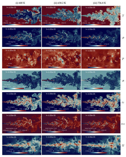
Figure 11.
Instantaneous contour plots obtained from simulations of n-dodecane injected at 200 m/s into a supercritical hot nitrogen, 972.9 K and 11.1 MPa, for various injection temperatures: first column 600 K, second column 658.2 K, third column 736.9 K. Rows, from top to bottom, show instantaneous fields of temperature T [K], density ], pressure p [Pa], dynamic viscosity ], specific heat at constant pressure cp [J/(kg K)], mole fraction of nitrogen xN2 [-], and velocity u [m/s].
Therefore, to examine quantitatively the mixing processes, the flow variables are averaged for about one flow-through time, and then normalized with respect to inlet conditions to make consistent comparisons. The centerline non-dimensional profiles of density, temperature, and velocity along with the normalized transverse mass flow rate are shown in Figure 12a–d, respectively. As for the cryogenic nitrogen case, these results indicate that at different injection temperatures, in the laminar jet region (x/d < 7) all the non-dimensional ratios present similar behavior. Beyond x/d = 8–10 the flow becomes turbulent (see Figure 11), and the increase in the jet temperature leads to a decrease of the density ratio, with a non-linear variation in the mass flow rate and slight fluctuations of the velocity profile.
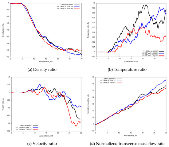
Figure 12.
Centerline axial profiles of non-dimensional density, temperature, velocity, and normalized transverse mass flow rate for different n-dodecane injection temperatures: 600 K, 658.2 K and 736.8 K. Simulations of n-dodecane injected at 200 m/s into a supercritical hot nitrogen, 972.9 K and 11.1 MPa.
The supercritical jet temperature case, at 736.8 K, shows small temperature fluctuations compared to the transcritical injection one at 600 K along the axial distance, as seen in Figure 12b. This is mainly due to decrease in the temperature gradient with reduced sensible heat transfer that occurs between the fuel jet and the surrounding hot nitrogen gas environment. The mixing index or normalized transverse mass flow rate is a non-linear function of the injection temperatures, as shown in Figure 12d, even if variations are rather small and maybe removable with a longer, but onerous, time averaging. Overall, the jet injection temperatures on non-dimensional mixing rate, quantified by the gas entrainment, show negligible effects, at least for the explored range of fluid temperatures.
Radial profiles are shown in Figure 13, displaying non-dimensional mean density, temperature and velocity at x/d = 20. These curves show a substantially independent width of the jets as the inlet temperature is varied, confirming the previous observation.
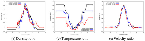
Figure 13.
Radial profiles of non-dimensional density, temperature, and velocity ratios at fixed axial distance x/d = 20, for different n-dodecane injection temperatures: 600 K, 658.2 K, and 736.8 K. Simulations of n-dodecane injected at 200 m/s into a supercritical hot nitrogen, 972.9 K and 11.1 MPa.
3.3.2. Effect of Chamber Pressure
The effect of chamber gas density is explored though different simulations carried out at increasing chamber pressure pch of 6 MPa, 11.1 MPa, and 30 MPa, with constant chamber temperature, Tch = 972.9 K, and using fixed n-dodecane inlet temperature, Tinj = 658.2 K. Figure 14 shows the comparison for the instantaneous contours of various flow variables for these cases. Results indicate that injecting n-dodecane fuel into a supercritical chamber leads to the formation of liquid-like jet structures of varying sizes. At low chamber pressure small scales are visible as in a pure atomization regime, while at high chamber pressure a transition towards gas-like phenomena is observed with larger scales and increased diffusive transport. In addition, an increased jet transverse spreading is also visible when moving from low to high chamber pressures.
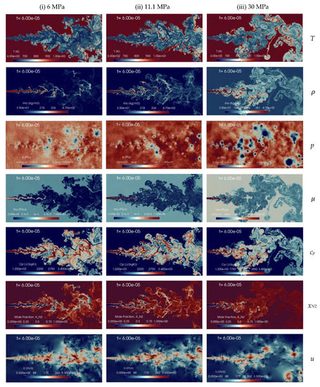
Figure 14.
Instantaneous contour plots obtained from simulations of n-dodecane injected at 658.2 K and 200 m/s into nitrogen at 972.9 K, for three different chamber pressures: first column 6 MPa, second column 11.1 MPa, third column 30 MPa. Rows, from top to bottom, show temperature T [K], density ], pressure p [Pa], dynamic viscosity ], specific heat at constant pressure cp [J/(kg K)], mole fraction of nitrogen xN2 [-], and velocity u [m/s].
For a quantitative examination of the mixing processes, the non-dimensional profiles of averaged properties in axial and radial directions are compared. The centerline non-dimensional profiles of density, temperature, velocity and the normalized transverse mass flow rate are shown in Figure 15a–d. Similar to the previous cryogenic cases, an intact jet core is observed for the n-dodecane injections, with centerline profiles not affected by the chamber pressure up to x/d ≤ 5. In the fully developed turbulent jet region, at axial distance x/d > 15, the increase of the supercritical chamber pressure level shows large effects in the variations of non-dimensional quantities along the axial length. The growth rate of the entrainment increases remarkably as chamber pressure levels increase, indicating a strong enhancement in the mixing rate due to chamber pressure (and therefore density). This, ultimately, means that higher chamber density promotes the multicomponent mixing process.
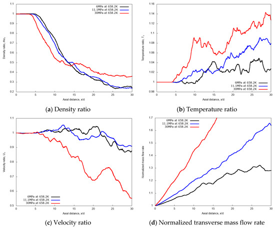
Figure 15.
Centerline axial profiles of non-dimensional density, temperature, velocity and normalized transverse mass flow rate for different chamber pressures: 6 MPa, 11.1 MPa, and 30 MPa. Simulations of n-dodecane injected at 658.2 K and 200 m/s into nitrogen at 972.9 K.
Figure 16 shows the radial variations of non-dimensional density, temperature and velocity profiles at the axial distance x/d = 20. Evidently, the density profile for the 30 MPa chamber pressure shows a broader spreading compared to 11.1 MPa and 6 MPa. Similarly, velocity radial profiles flatten as the pressure increases. Both aspects confirm the enhanced mixing at high chamber pressures.
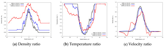
Figure 16.
Radial profiles of non-dimensional density, temperature and velocity at fixed axial distance x/d = 20, for different chamber pressures: 6 MPa, 11.1 MPa, and 30 MPa. Simulations of n-dodecane injected at 658.2 K and 200 m/s into nitrogen at 972.9 K.
3.3.3. Discussion
The investigations on the n-dodecane injection into nitrogen at trans- and supercritical conditions show an enhancement of the mixing rate as the chamber density increases, while they display a modest effect of the injected fuel properties variation. These results are in line with the previous investigation on the cryogenic nitrogen injection, therefore this allows to strengthen the conclusions. In the present case, the chamber pressure is varied by a large factor, up to 5 (30 MPa vs. 6 MPa), compared to the cryogenic nitrogen study, and larger variations are correspondingly observed. Likewise, the variation of the injected fluid density (from 532.5 kg/m3 to 412.2 kg/m3), explored through temperature changes (from 600.0 K to 736.8 K, respectively, at 11.1 MPa), causes minor effects on the injected mass based normalized mixing rate.
Overall, these findings can be useful for guiding future model developments and research directions, especially targeted towards 3D analysis of real supercritical combustors.
4. Conclusions
An advanced implicit LES model was developed to describe spray dynamics at trans- and super-critical conditions. Numerical simulations were carried out to investigate the fundamental characteristics of the evaporation, dispersion and multi-component species mixing processes, with emphasis on the quantitative assessment of gas entrainment. The new developed model includes real-fluid thermophysical properties and is implemented within the finite volume framework in the opensource software OpenFOAM. A pressure-based solver, using an extended segregated PIMPLE algorithm, proved to be able to handle large density ratios and highly non-linear thermophysical properties. The solver demonstrated the capability to couple species, energy, mass and momentum conservation equations in a stable manner.
The developed model was validated against the experimental studies of Mayer et al. [55] with good agreement. Subsequently, the effects of both injection temperature and chamber operating pressure conditions are evaluated through injections of cryogenic L-N2 and n-dodecane into a chamber filled with quiescent G-N2 environment. Qualitative analysis is performed for instantaneous solution fields, whereas quantitative aspects are discussed by examining non-dimensional averaged quantities, such as density, temperature, and velocity along axial or radial profiles, and by comparing normalized transverse mass flow rates along the axial distance. As a main finding of the study, for both cryogenic and diesel-like fuel injections, different chamber pressure conditions are found to affect the supercritical mixing processes more significantly than the injection temperatures. The present numerical study provides an insight of the jet behavior and the mixing processes at both trans- and super-critical conditions. Furthermore, the present numerical models demonstrated the capability to handle multicomponent species turbulent mixing processes with real-fluid thermophysical properties.
Author Contributions
Conceptualization, methodology and formal analysis, B.M.N., F.N.Z.R. and M.B.; software B.M.N., F.N.Z.R., M.B. and H.J.; validation and investigation, B.M.N. and F.N.Z.R.; writing—original draft preparation, B.M.N.; writing—review and editing, F.N.Z.R., M.B. and A.P.; supervision, M.B.; funding acquisition, H.G.I., H.J. and M.B. All authors have read and agreed to the published version of the manuscript.
Funding
This research was funded by the King Abdullah University of Science and Technology (KAUST), Saudi Arabia, under the CRG grant OSR-2017-CRG6-3409.03.
Acknowledgments
Authors gratefully acknowledge the SHAHEEN HPC facilities provided by KAUST.
Conflicts of Interest
The authors declare no conflict of interest. The funders had no role in the design of the study; in the collection, analyses, or interpretation of data; in the writing of the manuscript, or in the decision to publish the results.
References
- Dahms, R.N.; Oefelein, J.C. On the transition between two-phase and single-phase interface dynamics in multicomponent fluids at supercritical pressures. Phys. Fluids 2013, 25, 092103. [Google Scholar] [CrossRef]
- Jung, K.; Kim, Y.; Kim, N. Real-Fluid Modeling for Turbulent Mixing Processes of N-Dodecane Spray Jet Under Superciritical Pressure. Int. J. Automot. Technol. 2020, 21, 397–406. [Google Scholar] [CrossRef]
- Banuti, D.T. Crossing the Widom-line—Supercritical pseudo-boiling. J. Supercrit. Fluids 2015, 98, 12–16. [Google Scholar] [CrossRef]
- Ma, P.C.; Wu, H.; Banuti, D.T.; Ihme, M. Numerical analysis on mixing processes for transcritical real-fluid simulations. In Proceedings of the 55th AIAA Aerospace Sciences Meeting, Kissimmee, FL, USA, 8–12 January 2018. [Google Scholar] [CrossRef]
- Rodriguez, C.; Rokni, H.B.; Koukouvinis, P.; Gupta, A.; Gavaises, M. Complex multicomponent real-fluid thermodynamic model for high-pressure Diesel fuel injection. Fuel 2019, 257, 115888. [Google Scholar] [CrossRef]
- Taghizadeh, S.; Jarrahbashi, D. Proper orthogonal decomposition analysis of turbulent cryogenic liquid jet injection under transcritical and supercritical conditions. At. Sprays 2018, 28, 875–900. [Google Scholar] [CrossRef]
- Qiu, L.; Reitz, R.D. An investigation of thermodynamic states during high-pressure fuel injection using equilibrium thermodynamics. Int. J. Multiph. Flow 2015, 72, 24–38. [Google Scholar] [CrossRef]
- Branam, R.; Mayer, W. Length scales in cryogenic injection at supercritical pressure. Exp. Fluids 2002, 33, 422–428. [Google Scholar] [CrossRef]
- Chehroudi, B.; Talley, D.; Mayer, W.; Branam, R.; Smith, J.J.; Schik, A.; Oschwald, M.; Schick, A.; Oschwald, M. Understanding Injection into High Pressure Supercritical Environments. In Proceedings of the Fifth International Symposium on Space Propulsion, Chattanooga, TN, USA, 27–30 October 2003; pp. 1–37. [Google Scholar]
- Chehroudi, B.; Talley, D.; Coy, E. Visual characteristics and initial growth rates of round cryogenic jets at subcritical and supercritical pressures. Phys. Fluids 2002, 14, 850–861. [Google Scholar] [CrossRef]
- Ma, P.C.; Lv, Y.; Ihme, M. An entropy-stable hybrid scheme for simulations of transcritical real-fluid flows. J. Comput. Phys. 2017, 340, 330–357. [Google Scholar] [CrossRef]
- Müller, H.; Niedermeier, C.A.; Matheis, J.; Pfitzner, M.; Hickel, S. Large-eddy simulation of nitrogen injection at trans- and supercritical conditions. Phys. Fluids 2016, 28, 015102. [Google Scholar] [CrossRef]
- Rodriguez, C.; Vidal, A.; Koukouvinis, P.; Gavaises, M.; McHugh, M.A. Simulation of transcritical fluid jets using the PC-SAFT EoS. J. Comput. Phys. 2018, 374, 444–468. [Google Scholar] [CrossRef]
- Zhang, J.; Zhang, X.; Wang, T.; Hou, X. A numerical study on jet characteristics under different supercritical conditions for engine applications. Appl. Energy 2019, 252, 113428. [Google Scholar] [CrossRef]
- Ma, P.C.; Wu, H.; Jaravel, T.; Bravo, L.; Ihme, M. Large-eddy simulations of transcritical injection and auto-ignition using diffuse-interface method and finite-rate chemistry. Proc. Combust. Inst. 2019, 37, 3303–3310. [Google Scholar] [CrossRef]
- Ningegowda, B.M.; Rahantamialisoa, F.; Zembi, J.; Pandal, A.; Im, H.G.; Battistoni, M. Large Eddy Simulations of Supercritical and Transcritical Jet Flows Using Real Fluid Thermophysical Properties; SAE Technical Papers; SAE International: Warrendale, PA, USA, 2020; Volume 2020. [Google Scholar]
- Davis, D.W.; Chehroudi, B. Shear-coaxial jets from a rocket-like injector in a transverse acoustic field at high pressures. In Proceedings of the Collection of Technical Papers—44th AIAA Aerospace Sciences Meeting, Reno, NV, USA, 9–12 January 2006; Volume 13, pp. 9173–9190. [Google Scholar]
- Falgout, Z.; Rahm, M.; Sedarsky, D.; Linne, M. Gas/fuel jet interfaces under high pressures and temperatures. Fuel 2016, 168, 14–21. [Google Scholar] [CrossRef]
- Crua, C.; Manin, J.; Pickett, L.M. On the transcritical mixing of fuels at diesel engine conditions. Fuel 2017, 208, 535–548. [Google Scholar] [CrossRef]
- Segal, C.; Polikhov, S.A. Subcritical to supercritical mixing. Phys. Fluids 2008, 20, 052101. [Google Scholar] [CrossRef]
- Keser, R.; Ceschin, A.; Battistoni, M.; Im, H.G.; Jasak, H. Development of a Eulerian Multi-Fluid Solver for Dense Spray Applications in OpenFOAM. Energies 2020, 13, 4740. [Google Scholar] [CrossRef]
- Pandal, A.; García-Oliver, J.M.; Novella, R.; Pastor, J.M. A computational analysis of local flow for reacting Diesel sprays by means of an Eulerian CFD model. Int. J. Multiph. Flow 2018, 99, 257–272. [Google Scholar] [CrossRef]
- Desantes, J.M.; García-Oliver, J.M.; Pastor, J.M.; Olmeda, I.; Pandal, A.; Naud, B. LES Eulerian diffuse-interface modeling of fuel dense sprays near- and far-field. Int. J. Multiph. Flow 2020, 127, 103272. [Google Scholar] [CrossRef]
- Pandal, A.; Rahantamialisoa, F.; Ningegowda, B.M.; Battistoni, M. An Enhanced ς-Y Spray Atomization Model Accounting for Diffusion Due to Drift-Flux Velocities; SAE Technical Papers; SAE International: Warrendale, PA, USA, 2020; Volume 2020. [Google Scholar]
- Xue, Q.; Battistoni, M.; Powell, C.F.; Longman, D.E.; Quan, S.P.; Pomraning, E.; Senecal, P.K.; Schmidt, D.P.; Som, S. An Eulerian CFD model and X-ray radiography for coupled nozzle flow and spray in internal combustion engines. Int. J. Multiph. Flow 2015, 70, 77–88. [Google Scholar] [CrossRef]
- Battistoni, M.; Magnotti, G.M.; Genzale, C.L.; Arienti, M.; Matusik, K.E.; Duke, D.J.; Giraldo, J.; Ilavsky, J.; Kastengren, A.L.; Powell, C.F.; et al. Experimental and Computational Investigation of Subcritical Near-Nozzle Spray Structure and Primary Atomization in the Engine Combustion Network Spray D. SAE Int. J. Fuel Lubr. 2018, 11, 337–352. [Google Scholar] [CrossRef]
- Lebas, R.; Menard, T.; Beau, P.A.; Berlemont, A.; Demoulin, F.X. Numerical simulation of primary break-up and atomization: DNS and modelling study. Int. J. Multiph. Flow 2009, 35, 247–260. [Google Scholar] [CrossRef]
- Ménard, T.; Tanguy, S.; Berlemont, A. Coupling level set/VOF/ghost fluid methods: Validation and application to 3D simulation of the primary break-up of a liquid jet. Int. J. Multiph. Flow 2007, 33, 510–524. [Google Scholar] [CrossRef]
- Ningegowda, B.M.; Premachandran, B. A Coupled Level Set and Volume of Fluid method with multi-directional advection algorithms for two-phase flows with and without phase change. Int. J. Heat Mass Transf. 2014, 79, 532–550. [Google Scholar] [CrossRef]
- Ningegowda, B.M.; Premachandran, B. Numerical investigation of the pool film boiling of water and R134a over a horizontal surface at near-critical conditions. Numer. Heat Transf. Part A Appl. 2017, 71, 44–71. [Google Scholar] [CrossRef]
- Ningegowda, B.M.; Premachandran, B. Free convection film boiling over a discrete flat heater with different surface orientations. Numer. Heat Transf. Part A Appl. 2019, 76, 712–723. [Google Scholar] [CrossRef]
- Ningegowda, B.M.; Premachandran, B. Saturated film boiling of water over a finite size heater. Int. J. Therm. Sci. 2019, 135, 417–433. [Google Scholar] [CrossRef]
- Ningegowda, B.M.; Ge, Z.; Lupo, G.; Brandt, L.; Duwig, C. A mass-preserving interface-correction level set/ghost fluid method for modeling of three-dimensional boiling flows. Int. J. Heat Mass Transf. 2020, 162, 120382. [Google Scholar] [CrossRef]
- Jofre, L.; Urzay, J. Transcritical diffuse-interface hydrodynamics of propellants in high-pressure combustors of chemical propulsion systems. Prog. Energy Combust. Sci. 2021, 82, 100877. [Google Scholar] [CrossRef]
- Bellan, J. Direct numerical simulation of a high-pressure turbulent reacting temporal mixing layer. Combust. Flame 2017, 176, 245–262. [Google Scholar] [CrossRef]
- Yi, P.; Yang, S.; Habchi, C.; Lugo, R. A multicomponent real-fluid fully compressible four-equation model for two-phase flow with phase change. Phys. Fluids 2019, 31, 026102. [Google Scholar] [CrossRef]
- Yang, S.; Yi, P.; Habchi, C. Real-fluid injection modeling and LES simulation of the ECN Spray A injector using a fully compressible two-phase flow approach. Int. J. Multiph. Flow 2020, 122, 103145. [Google Scholar] [CrossRef]
- Yang, S.; Habchi, C. Real-fluid phase transition in cavitation modeling considering dissolved non-condensable gas. Phys. Fluids 2020, 32, 032102. [Google Scholar] [CrossRef]
- Zong, N.; Yang, V. Cryogenic fluid jets and mixing layers in transcritical and supercritical environments. Combust. Sci. Technol. 2006, 178, 193–227. [Google Scholar] [CrossRef]
- Gopal, J.M.; Tretola, G.; Morgan, R.; de Sercey, G.; Atkins, A.; Vogiatzaki, K. Understanding Sub and Supercritical Cryogenic Fluid Dynamics in Conditions Relevant to Novel Ultra Low Emission Engines. Energies 2020, 13, 3038. [Google Scholar] [CrossRef]
- Irannejad, A.; Banaeizadeh, A.; Jaberi, F. Large eddy simulation of turbulent spray combustion. Combust. Flame 2015, 162, 431–450. [Google Scholar] [CrossRef]
- Ghosh, S.; Hunt, J.C.R. Induced air velocity within droplet driven sprays. Proc. R. Soc. Lond. Ser. A Math. Phys. Sci. 1994, 444, 105–127. [Google Scholar] [CrossRef]
- Siebers, D.L. Liquid-Phase Fuel Penetration in Diesel Sprays. SAE Trans. 1998, 107, 1205–1227. [Google Scholar]
- Pickett, L.M.; Siebers, D.L. Orifice diameter effects on diesel fuel jet flame structure. J. Eng. Gas Turbines Power 2005, 127, 187–196. [Google Scholar] [CrossRef]
- Sepret, V.; Bazile, R.; Marchal, M.; Couteau, G. Effect of ambient density and orifice diameter on gas entrainment by a single-hole diesel spray. Exp. Fluids 2010, 49, 1293–1305. [Google Scholar] [CrossRef]
- Matheis, J.; Hickel, S. Multi-component vapor-liquid equilibrium model for LES of high-pressure fuel injection and application to ECN Spray A. Int. J. Multiph. Flow 2018, 99, 294–311. [Google Scholar] [CrossRef]
- Chungó Mohammad Ajlan, T.-H.; Lee, L.L.; Starling, K.E. Generalized Multiparameter Correlation for Nonpolar and Polar Fluid Transport Properties. Ind. Eng. Chem. Res. 1988, 27, 671–679. [Google Scholar]
- Jarczyk, M.; Pfitzner, M. Large eddy simulation of supercritical nitrogen jets. In Proceedings of the 50th AIAA Aerospace Sciences Meeting Including the New Horizons Forum and Aerospace Exposition, Nashville, TN, USA, 9–12 January 2012. [Google Scholar]
- Poling, B.E.; Prausnitz, J.M.; O’connell, J.P.; York, N.; San, C.; Lisbon, F.; Madrid, L.; City, M.; Delhi, M.N.; Juan, S. The Properties of Gases and Liquids, 5th ed.; McGraw Hill: New York, NY, USA, 2001. [Google Scholar] [CrossRef]
- Petit, X.; Ribert, G.; Lartigue, G.; Domingo, P. Large-eddy simulation of supercritical fluid injection. J. Supercrit. Fluids 2013, 84, 61–73. [Google Scholar] [CrossRef]
- Banuti, D.T.; Ma, P.C.; Hickey, J.P.; Ihme, M. Thermodynamic structure of supercritical LOX-GH2 diffusion flames. Combust. Flame 2018, 196, 364–376. [Google Scholar] [CrossRef]
- NASA. Polynomials. Available online: http://combustion.berkeley.edu/gri-mech/data/nasa_plnm.html (accessed on 19 October 2020).
- Kim, T.; Kim, Y.; Kim, S.K. Numerical study of cryogenic liquid nitrogen jets at supercritical pressures. J. Supercrit. Fluids 2011, 56, 152–163. [Google Scholar] [CrossRef]
- Thermophysical Properties of Fluid Systems. Available online: https://webbook.nist.gov/chemistry/fluid/ (accessed on 18 October 2020).
- Mayer, W.; Telaar, J.; Branam, R.; Schneider, G.; Hussong, J. Raman measurements of cryogenic injection at supercritical pressure. Heat Mass Transf. und Stoffuebertragung 2003, 39, 709–719. [Google Scholar] [CrossRef]
- Engine Combustion Network|Engine Combustion Network Website. Available online: https://ecn.sandia.gov/ (accessed on 14 September 2020).
- Rodriguez, C.; Koukouvinis, P.; Gavaises, M. Simulation of supercritical diesel jets using the PC-SAFT EoS. J. Supercrit. Fluids 2019, 145, 48–65. [Google Scholar] [CrossRef]


Publisher’s Note: MDPI stays neutral with regard to jurisdictional claims in published maps and institutional affiliations. |
© 2020 by the authors. Licensee MDPI, Basel, Switzerland. This article is an open access article distributed under the terms and conditions of the Creative Commons Attribution (CC BY) license (http://creativecommons.org/licenses/by/4.0/).