1. Introduction
Non-Technical Losses (abbreviated as NTL) refers to all losses caused by utility theft: meter tampering, bypassing meters, faulty or broken meters, un-metered supply or technical and human errors in meter readings [
1]. According to a study of Northeast Group, NTL is quantified in US
$ 96 billion per year, globally [
2]. Therefore, reducing NTL is one of the top priorities of utility companies.
A well-known strategy to fight NTL is to visit customers regularly to check whether the client is committing fraudulent activities. Since visiting each customer is expensive, utility companies generate campaigns (a campaign is a small, selected subset of clients which the company decided to inspect, these clients are often in the same region and have the same tariff) visiting those customers that might be suspicious (e.g., customers with low consumption in a long period). A common approach to determine which customers are suspicious of committing frauds (or with any type of energy loss) is to build a supervised system that exploits the historical data available in their systems.
The challenge of implementing a good supervised system to detect NTL is significant. On the one hand, there are several data-related problems. It is well known that having labelled instances properly representing the domain is a key aspect to building robust supervised methods. However, the labelled instances are usually biased (e.g., the companies over-control the customers that have committed several times fraud, or generate more campaigns on those regions in which they have historically detected more fraud). On the one hand, there is the well-known trade-off problem between using a black-box algorithm (e.g., ensemble or deep learning algorithms), that should provide better NTL detection results, and using a simpler algorithm that would be easier to interpret for the stakeholder (e.g., linear regression or decision trees). Moreover, complex algorithms like ensembles or deep learning are harder to implement compared to simpler alternatives. In general, as explained in
Section 2.2, the literature tends to use the black-box and complex algorithms to implement supervised solutions. However, the selection of the complex algorithms over the interpretable ones presents a challenge for stakeholders, since they cannot validate the models learnt nor the campaigns done.
Despite the magnitude of the challenge, we have been able to achieve good results over different campaigns for one of the largest gas and electricity providers in Spain [
3]. Our system has achieved good results in electricity and gas campaigns. In electricity, we have achieved campaigns with higher than 50% of accuracy for customers with no contract, and up to 36% in customers with a contract, a very high proportion considering the very low percentage achieved by the company with the former approaches in Spain, a region with a very low proportion of fraud. These good results are partly a consequence of our efforts dealing with the problems previously explained. For instance, in [
4] we show how segmenting campaigns by region helps to mitigate some of the biases, and in [
5] we explain our first effort to provide explainable results using local explanations [
6]. We find, however, that there is room for improvement: our previous system lacks consistency in terms of accuracy (i.e., we obtain a mix of very good campaigns with other campaigns with fair results).
In this paper, we extend our system in two ways. First, we incorporate the Shapley values [
7] in our system, that provides a trustworthy modular explanation. It helps to analyse the correctness of the model both to the scientists (e.g., to detect undesired patterns learnt) and the stakeholders (that can understand the black-box algorithm, and their role in generating campaigns is therefore significantly augmented). Second, we evidence, though different experiments, how segmenting the labelled data according to the feedback notified by the technician (i.e., the type of meter problem that causes the energy loss) into several simpler models improves both the accuracy, but also the explanation capabilities of our state-of-the-art explainer technique.
The remainder of this paper has the following structure: in
Section 2 we briefly describe our NTL system and compare it with other similar work in the literature.
Section 3 and
Section 4 present advances and results in real-case scenarios. The paper is concluded in
Section 5 with the conclusions and future work.
2. Non-Technical Loss Systems in the Literature
2.1. Our Approach
Our NTL framework implements a supervised classification model that learns from historical cases of NTL. Our system is autonomous (it generates campaigns with minimum human interaction), versatile (it can be used for different types of energy and/or customers), and incremental (results from previous campaigns are used as feedback to improve future performance). It is already in production and has been explained in previous work [
3,
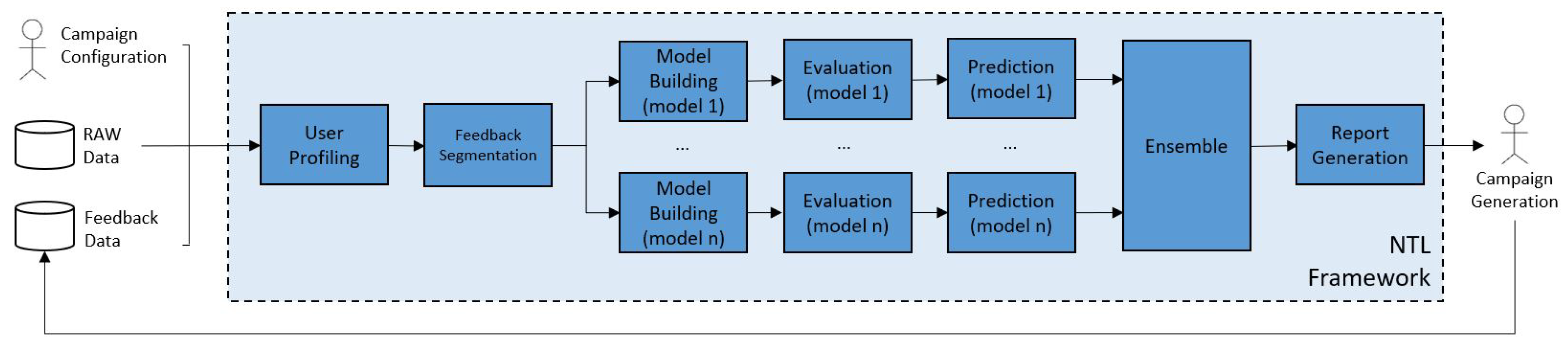
4]. The process of detecting NTL can be summarized as follows (see
Figure 1):
Campaign Configuration. The stakeholder delimits the segmentation of the campaign, namely: utility type, region and tariff.
User Profiling. When the configuration is set, appropriate data is extracted from the company (mostly consumption information but also static data such as tariff or meter location) as well as other external open data (climate and socioeconomic data). With this information, historical client profiles are built (which constitutes the labeled information) and current profiles (current month) which determine the prediction set.
Model Building and Evaluation. We build a Gradient Boosting model classifier. The number of boosted trees included in the model is set by a training validation analysis of 80–20%.
Prediction. With the model trained with all the data we assign a score to each customer from the campaign configuration.
Report Generation. The top-scoring customers are included in a report with complementary information (e.g., whether the customer has been visited recently). This information is used by stakeholders to determine which customers should be included in the campaign.
Campaign Generation. Technicians visit the high scoring customers included in the campaign, and the results of the visit (i.e., whether the customer is an actual NTL case), as well as the characteristics of the NTL case (e.g., if the customer manipulated the meter, or if it was just a malfunction of the meter), are recorded. This new feedback is stored for future campaigns (feedback manipulation).
Using Gradient Boosting presents several advantages over other modelling techniques. We list some of them:
Modern implementations of classical tree boosting (i.e., XGboost, LightGBM and CatBoost) offer a good trade-off between accuracy and ease of use, especially with tabular data (in comparison to other alternatives such as Deep Learning or Support Vector Machines that require specific preprocessing for each domain).
These algorithms tend to be very accurate with little parameter tuning. In our case, it is tuned to the number of individual trees that are included in the final model and optimized with cross-validation. To tune the other main hyperparameter, i.e., learning rate, it is used the CatBoost heuristic based on the input training data (nr. of rows and columns). Furthermore, we use bagging (i.e., subsample of 0.66 in each tree) to reduce the well-known problem of high variance from decision tree models.
Using decision trees allows us to take advantage of the TreeShap implementation which computes Shapley values significantly faster (reducing time from exponential to polynomial) [
8].
The system has been used to generate campaigns in gas (6 million customers) and electricity (4 million customers), in small customers (e.g., apartments), industries, customers with contract and historical customers without an active contract. For each case, we have engineered the features to fit the segment (depending on the segment we have up to several hundred features). For instance, in the customers without an active contract, the consumption features focus on the consumption behavior during the last months of the contract, in contrast with the customers with a contract that has much different consumption information both to reflect the historical consumption and its behavior at present.
The framework has been built using Python and dedicated Machine-Learning libraries such as pandas, scikit-learn, XGBoost, CatBoost and LightGBM. Overall, the features can be summarized as follows:
Consumption data. Features related to the consumption of the customer. It includes raw information (i.e., the consumption in kWh for a period of time), features measuring changes in the consumption of the customer (e.g., abrupt decrease of consumption), as well as features that compare the consumption of the customer against other similar customers (e.g., values that scores the similarity between the consumption curve of the customer and the average consumption). These are the most important features in our supervised system since they should reflect the consumption behavior of a customer that incurs into NTL.
Static data. Information related to the client typology, for instance, the type of meter or the tariff. Furthermore, the street address is included in the study allowing the detection of areas with historical loses.
Visits data. Features profiles whether the customer has been visited, how many times the customer committed fraud or how many months have passed since the last visit done to that customer, among other related information.
Sociological data. It includes information such as the town and province where the customer lives.
Additionally, we complement sociological data from external Open Data sources. The addition of this contextual information aims to counter possible biases introduced when dealing with a population with different socioeconomic status or weather conditions. These features are summarized as follows:
2.2. Related Work
Non-technical loss detection is a popular subfield of fraud detection that has received a significant amount of attention. It presents serious challenges which we list below. Class Imbalance; fraudulent cases are scarce in comparison to non-fraudulent ones. Dataset Shift; i.e., training (historical) data may not be representative of the future. Scalability; solutions must work for small-sized campaigns up to campaigns with millions of customer profiles in an acceptable execution time [
1].
In electricity, many of the approaches are similar to our framework in the sense that they implement supervised machine-learning techniques; here, we list a representative few. M. Buzau et al. [
9], presents a framework sharing many elements to our approach: it uses XGBoost algorithm, is implemented for a utility company in Spain and the experiments reported are performed using real data. On the other hand, its authors address the project using smart meter measurements (automatic readings), whereas in our case, the dataset is from measurements reported manually by the client. The authors report a hit-rate of around 20%.
Most of the other related work focuses on the usage of Discriminate models. In [
10] the authors propose an automatic feature extraction engine combined with Support Vector Machine (SVM) capable of analyzing nearby 300,000 clients in the Asian market with a hit-rate of 37%. In [
11] is another successful example using Optimal-Path Forests (OPF) classifier, the authors use data from a Brazilian utility company and report an accuracy of 86%, the hit-rate is not reported.
In [
12] proposed an end-to-end NTL framework based on Neural Network techniques, the authors implement a multilayer perceptron (MLP). They reported experiments using real data from Brazil achieving an F1-score of 40%. Furthermore, in [
13] is another example of using Neural Networks with the advantage of no definition of explicit features. Using Neural Networks, the framework aims to capture the internal characteristics and correlation of consumption to point out outlier clients. The method proposed achieves an F1-score of 92% using synthetic data.
One of the few examples of developing an NTL for other types of utilities is the following: ref. [
14] presents a set of analysis to detect meter tampering in the water network. The authors proposed a two-step algorithm to detect abnormalities in the network. First, using the Pearson correlation are detected clients with negative correlation. After the clients are filtered using expert system rules. Using this algorithm, the authors detected nearby 7% of total meter tampering issues.
Other approaches use unsupervised methods to detect outlier profiles and therefore potentially fraudulent activities. For instance, ref. [
15] propose a two-step algorithm: the customers are clustered according to the consumption and after that potential fraudsters are scored using a unitary index score. In [
16] the authors use the analysis of time series to detect irregularities in customer behavior. Furthermore, in [
17] proposed Self-organizing maps to compare historical and current consumption to show possible frauds.
In contrast to much existing related work that provides results on specific domains with a high proportion of NTL, our work has focused on mitigating the long-term challenges of implementing an NTL detection system in a region with a low proportion of NTL. The contribution of this work is the following: first, we are the very first to implement the Shapley values to understand the correctness of the system beyond benchmarking. Second, we demonstrate that segmenting the customers according to their type of NTL, oversampling the cases and combining them with a bucket of models helps the system to improve accuracy.
3. Methodology
In this work, we propose to convert our previous system that builds a unique global model into a system that uses a bucket-of-models (where each model is used specifically to score one type of NTL), to improve the robustness and accuracy of the campaign. The process (illustrated in
Figure 2), segments the data according to the NTL case reported by the stakeholder (see
Section 3.1). To mitigate the high imbalance in our data we make use of oversampling (see
Section 3.2) which creates new synthetic samples of the minority class thus reducing the imbalance. Then, an independent pipeline for each segmented dataset is created and the models generated are finally combined using a bucket-of-models approach (see
Section 3.3). Finally, the explainability proxy provides explanations (see
Section 3.4).
3.1. Segmentation
Our first improvement consists of building better campaigns by converting our catch-all system into a combination of specific models. As explained in
Section 1, if the technician detects a fraudulent customer (or had an NTL), it includes in the report how the NTL has been committed. The NTL cases can be grouped in three non-overlapping categories: Meter Tampering (referred as
), Bypassing Meters (
) and Faults (
).
Each NTL, as seen in
Table 1, has unique characteristics (e.g., a bypassed meter would not register any type of energy consumption, while the other two types of NTL might still detect a lower consumption). Therefore, how these NTL cases are reflected in our features differs. Hence, we aim to build specific models for each NTL case, particularizing the learning of orthogonal and possibly independent NTL patterns.
3.2. Oversampling
As with any fraud detection system, the data available is highly imbalanced. The problem is aggravated due to the segmentation of the minority class into three individual groups while keeping all non-NTL cases in each group. To deal with this extreme case of imbalance, oversampling is applied to under-represented NTL instances. We use two popular variants of oversampling: SMOTE (Synthetic Minority Oversampling Technique) [
18] and ADASYN (Adaptive Synthetic Sampling) [
19]. SMOTE creates new instances adding points between positive and negative instances (using k-nearest neighbors). ADASYN is similar but slightly more sophisticated in that it tends to generate new points in the more difficult regions near class borders.
Section 4 compares results with and without balancing, showing that in many cases it is indeed very useful.
3.3. Model Building
After dividing the NTL cases into different groups, we build specific models for each segment and choose the best one. This strategy, known as a bucket of models, is generally able to learn better patterns and therefore, improve the accuracy. The bucket of models is an ensemble approach in which different models are available and the ensemble uses for each problem, the model that shows more promising performance. This naive explanation, in our NTL, consists of having three NTL models—one for each NTL type—that will score each customer independently. The final score of each customer corresponds to the highest score assigned by one of these models, i.e., if
x is the instance to be scored, and
the model specialized in detecting fraud by Meter tampering,
the model specialized in detecting the fraud by Bypassing meters, and
the model that detects the other non-fraudulent NTL, the final score assigned to
x,
is given by:
The maximum score is used, since each model is independent and, as already mentioned, it is specialized in one type of NTL. For instance, a customer that had a 0.8 score in one model and 0.1 in the other two is more suspicious than one that had for each model 0.33.
3.4. Report Building
In addition to the information already included in the campaigns, we provide an individual explanation for each client in the report using the Shapley Additive exPlanations (SHAP) library [
7].
This library is a state-of-the-art model-agnostic method that explains the predictions as a cooperative game using Shapley values made by a machine-learning algorithm, in our case from the Gradient boosting model [
20].
The previous formula shows the definition of the Shapley values of a feature j in instance x, where p is the number of features, S corresponds to subsets of features, and the function indicates the prediction for different combinations of features. The difference between the values indicates how the prediction changes (i.e., the marginal value) after adding a particular feature to S. The sum is over all possible subsets S that can be built without including . Finally, corresponds to a normalizing factor that takes into account all the permutations that can be made with subset size , to distribute the marginal values among all the features of the instance. The use of SHAP can be summarized in our case as follows:
Our supervised model assigns a score .
SHAP computes the Shapley values and the base value:
Adding up the base value and the Shapley values of an instance, we obtain the final score. In the Catboost classification model, both the Base Value and the Shapley values correspond to a raw value; the sigmoid of that value corresponds to the true probability.
Including the SHAP values in our system, provides two benefits. First, we aim to better understand the model learnt, a knowledge that should help us improve and evaluate our system (e.g., performing better feature engineering, or modifying the parameter configuration). Second, the stakeholder should have better control of the campaigns built (for instance, the user may want to modify the size of campaigns depending on the trustworthiness provided by the SHAP explanations).
4. Tests
To evaluate the benefits of the ensemble proposal (referred as
) over the baseline model (
, the model without the bucket of models explained in
Section 3), the following aspects are considered: Accuracy Preservation, Singularity and Explainability Enhancement. The tests are performed over different datasets that actually taken from real campaigns: they constitute successful campaigns done in the past with the previous system, but still show room for improvements. Please see [
4] for a full explanation of the success of our campaigns: we have achieved campaigns of around 50%, and also a large amount of energy recovered. These campaigns are briefly described as follows:
Campaign 1: Campaign aimed to detect NTL in customers with long periods of no consumption and with the most common domestic tariff.
Campaign 2: Campaign performed in a very populated but quite scattered region (i.e., with many towns with small populations). This campaign aimed to detect all types of customers from the most common tariff.
Campaign 3: Campaign designed to detect NTL in non-contracted customers (i.e., customers that had a contract that was interrupted) with high contracted power (i.e., industrial clients and manufacturers).
4.1. Accuracy Preservation
To show an improvement of the ensemble model
(Bucket, Bucket + SMOTE, Bucket + ADASYN) over the baseline model
it should be the case that
ranks fraudulent customers higher than
. In our system, Average Precision score (
) is used to benchmark the performance of a model [
21]. As the precision-recall curve the plot shows the trade-off between precision and recall for different thresholds, the Average Precision summarizes the precision-recall curve as the weighted mean of precision achieved at each threshold, with the increase in recall from the previous threshold used as the weight:
Here,
denotes recall at rank position
n (i.e., the fraction of fraudulent cases in the dataset that are actually retrieved), and
denotes precision at rank position
n (i.e., the fraction of retrieved instances at threshold
n that are indeed fraudulent). This metric is similar to the Area Under the Curve (AUC) metric, but should be preferred when only focusing on the position of the positive labeled instances, which is the case here [
22].
The results of our benchmark analysis can be found in
Table 2. The methods compared are Baseline (our previous system w/o balancing or segmentation), Bucket (with segmentation of NTL cases and balancing obtained through undersampling of the majority class), Bucket + SMOTE (SMOTE balancing and segmentation), and Bucket + ADASYN (ADASYN balancing and segmentation). In all cases, the ensemble approach clearly outperforms the baseline approach.
The best method is Bucket + SMOTE for Campaign 1 and 3, and Bucket + ADASYN for Campaign 2. They clearly improve the results of two campaigns while maintaining the results of the second one (see
Table 3). Considering that many of the customers with high score were not included in the original campaign, the process of evaluating the success of the ensemble model is specified as follows:
The ensemble model is built and used to score all the customers (i.e., the customers included in the campaign, and the others).
The top N customers are selected, where N is the same number of customers selected in the original campaign.
For each customer selected, it is assigned the following as the result in the campaign:
- (a)
If the customer was visited in the original campaign, the result is the same.
- (b)
If the customer was not visited in that campaign, but visited in the following months, we select the result of the future campaign as a result in the current campaign.
- (c)
If the customer was visited neither in that campaign nor in the future campaign, despite that we do not know if the customer is committing NTL, it is included in our results as a non-NTL.
4.2. Visualizing Singularity
The individual models from the ensemble should be used to learn unique patterns from singular instances. Where
are the models from the ensemble model and
the unique characteristics that define the group of instances:
The main purpose of converting our unique catch-all model that aims to detect all types of NTL cases into an ensemble bucket of models, is to facilitate the learning process of each NTL: If each model focuses on one type of NTL, it should be easier to extract the patterns that define the NTL. The consequence of learning unique patterns is that we should increase global accuracy.
To analyze this property, we propose to visualize through the t-SNE method [
23]. This technique allows the representation of high-dimensional data into two dimensions (a non-linear dimensionality reduction is applied) where similar observations are represented nearby and dissimilar appear distant.
In our case, if the individual models from the ensemble learn unique patterns, the Shapley values should also be unique (i.e., each model should learn differently) and therefore, it should be reflected in the t-SNE plot appearing distant clusters.
Figure 3 includes the t-SNE representations for Shapley values of predicted clients in Campaigns 1–3. As we can observe the representations for campaigns using segmentation are grouped in the same clusters for the data used in the experiments.
4.3. Explainability Enhancement
The explanations obtained through the explainer method (in our case, using SHAP) from the ensemble model should be better than the baseline. A better explanation can be defined as the agreement of the explanation using expert knowledge:
The explainer methods have proven to be useful for understanding how a model was learnt (and why an instance has received a specific score); if we obtain an explanation of our machine-learning model, we can evaluate the correctness according to human knowledge (e.g., the stakeholder in charge of the detection of NTL in the company). This process is facilitated by the ensemble model: each model learns one type of NTL, therefore the explanation of each model for the datasets considered was simpler yet better and easier to understand. To analyze explanations, we face the problem of analyzing the quality of an explanation when there is no formal methodology [
24]. For this work, we will use the trend to evaluate the explainability using an abstraction of what the model was predicted. This allows us to obtain an explanation while we work with very accurate black-box algorithms. The methods used to compare the explanation of the models are the Goodness of our model (the deeper analysis of the expert stakeholder) and Oracle Querying (a rule system that aims to simulate the analysis of the stakeholder). In each case, we will use the Shapley values from SHAP already explained in
Section 3.4.
4.3.1. Previous Analysis: When Is a Model Trustworthy
In general, we consider a model good if it bases its predictions on features that tend to change when the customer commits an NTL. These include mostly the consumption features (e.g., a customer that commits fraud will have an abrupt decrease of consumption), but also other features that are highly related with abnormal consumption behavior (e.g., the absences of readings, i.e., if the company does not receive meter readings from the customer it might be a consequence of a meter manipulation).
The other features, in general, are considered complementary; the town where the customer lives can nuance all the instances according to historical knowledge (i.e., a customer that lives in a town where the company usually detected NTL, the town feature should increase the final score of that customer), or the features related to the visits, which can be useful to detect recidivist customers, but we consider that a model than only bases on this complementary information is biased and might be subject of dataset shift.
4.3.2. Goodness of Our Model
An option to determine whether an explanation is trustworthy is to plot the feature contribution of predicted instances and obtain an expert evaluation. The analysis is done by computing the average of the Shapley values for the predicted customers. This analysis provides a global vision of how the model learnt, which is useful to determine its quality.
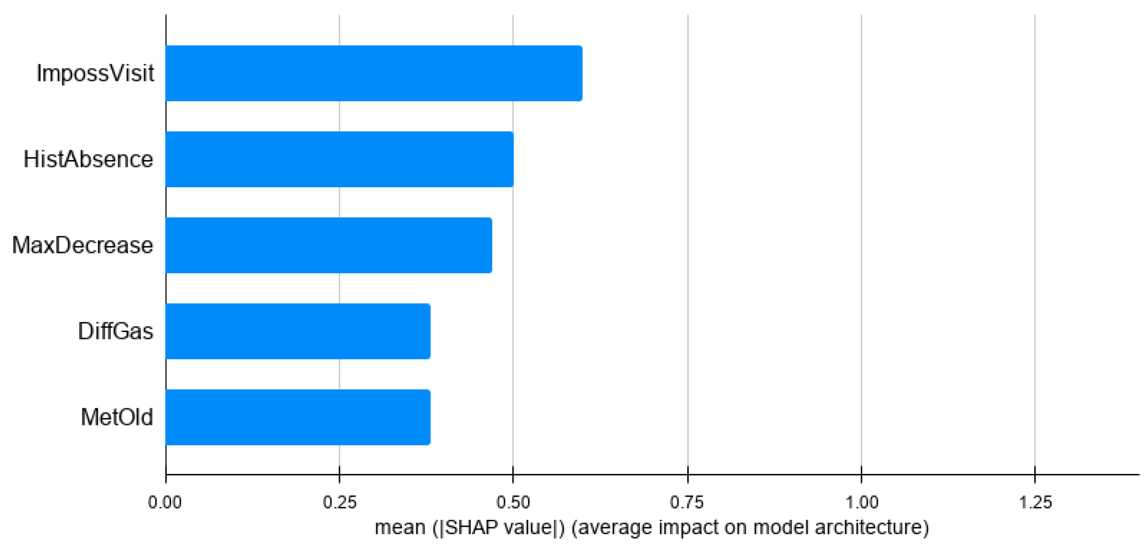
Figure 4 shows the top 5 most important features for the baseline model and
Figure 5,
Figure 6 and
Figure 7 include the top contributing features of individual models of the ensemble approach.
In
Figure 4, it can be observed that the features are related and useful to detect NTL, but it seems to be a catch-all model. There are different types of features: a consumption-related feature, a meter feature, a visit feature, an absence feature and a gas feature.
For the Bypassing Meter model (see
Figure 5), we can see that it includes more consumption feature information: this is indeed expected, since the meter tampering should be reflected in an abrupt decrease in consumption.
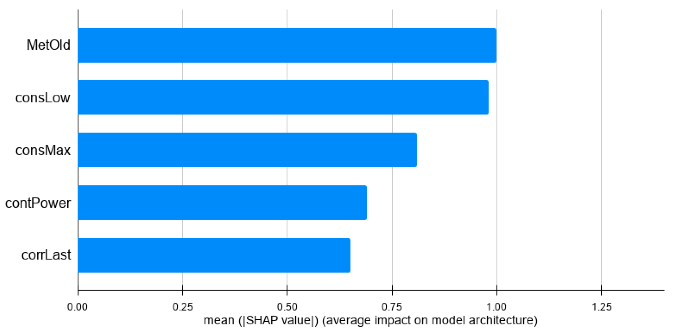
For the Faults model (see
Figure 6), we observe information related to the consumption as well. This is expected since malfunction of a meter should be reflected in the consumption behavior. However, we obtain additional interesting features specific to this model: first, the fact that the most important feature for this model is the age of the meter (older meters tend break more). Second, the fact that the last correct visit is the fifth most important feature (i.e., a recently revised meter should not be faulty).
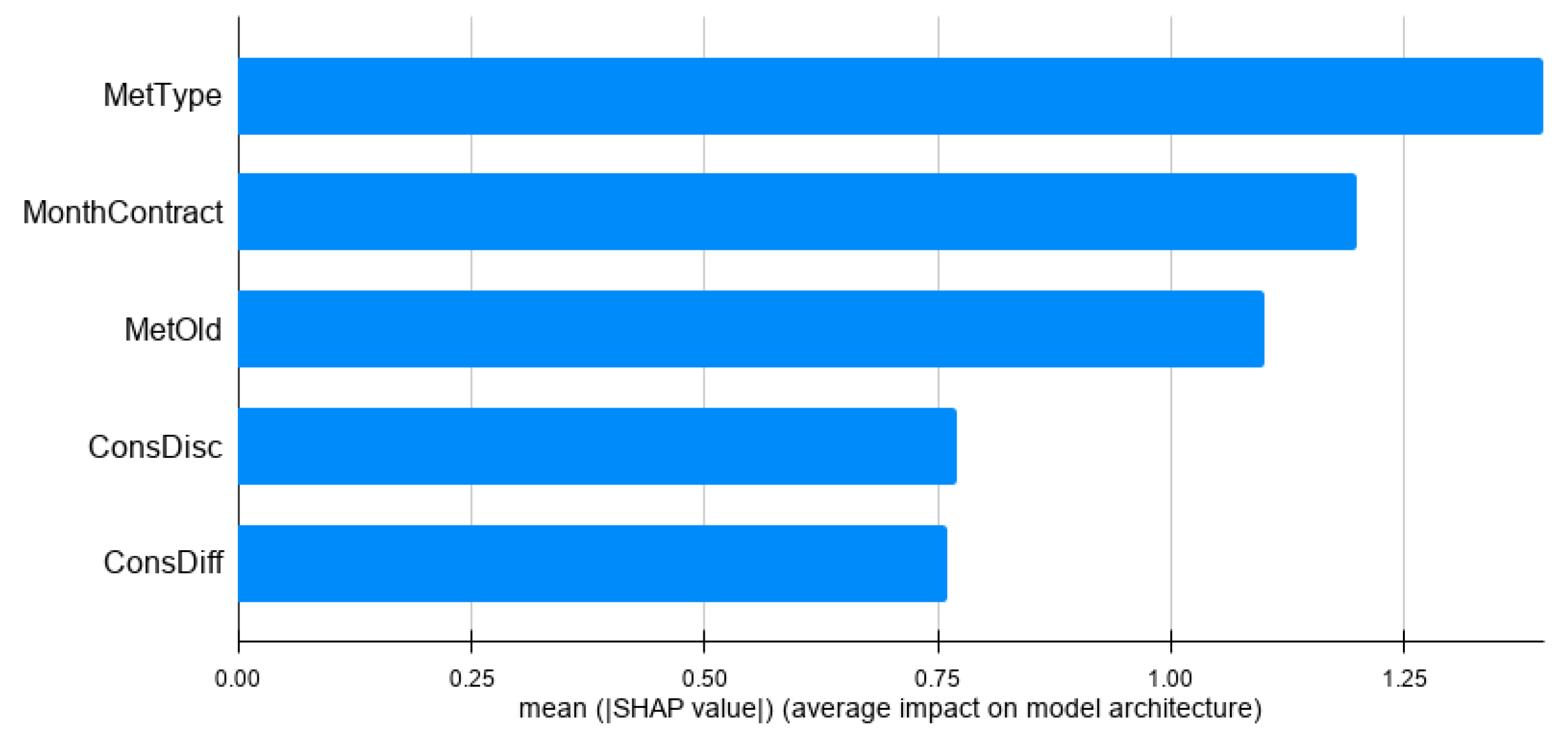
Finally, the Meter tampering model (see
Figure 7) also includes several consumption features, but there is one specific feature that is relevant for this specific model: the binary
met_typ feature that indicates if a meter is smart. This is extremely relevant since this campaign was done when the company was updating the meters and installing smart meters which are more difficult to manipulate, and it can even warn the company if it detects that it is being manipulated.
In summary, each model learns different patterns that better reflect the characteristics of each NTL for the datasets considered. We find this fact very reassuring in the sense that it supports our belief that our system is working properly and capturing essential information in each of the NTL segments.
4.3.3. Oracle Querying
This technique is based on a rule system that mimics the behavior of the stakeholder by automatically evaluating each local explanation using rules. Depending on the agreement (i.e., the agreement that the stakeholder has in the explanation, see
Section 4.3.2), the customer would be included or discarded in the final campaign. We have formulated rules to compute the agreement and to evaluate the oracle-querying system. The process can be summarized as follows:
For each predicted instance included in a campaign:
Compute the top 5 contributing features using SHAP.
Execute oracle querying using the following rules:
Consumption rule: Any of the top 5 features is consumption-related (e.g., abrupt decrease of consumption).
Risk rule: Any of the top 5 features are risk or poverty-related (e.g., the customer lives in a town with very high unemployment).
If any of the top five contributing features pass the rules defined, the explanation is considered trustworthy.
The agreement is computed as the proportion of customers that pass this oracle-querying process. As
Table 4 shows, the agreement is improved using the ensemble model in the first two campaigns and maintains the results in the last one.
5. Conclusions
In this paper, we propose several extensions to a machine-learning-based NTL detection system. Our aim is to increase the accuracy of our NTL detection system, by generating very specific models for each NTL typology, oversampling the minority class and combining them using a bucket of models. This approach improves the overall quality of our predictions for the datasets considered since it helps our models to focus on specific, more homogeneous patterns. We plan as future work to corroborate these findings with a more thorough analysis and experiments.
In addition, the segmented approach also improves the interpretability of the derived models, a mandatory requirement in the context of industrial projects where non-technical Stakeholders may be involved. In this work, we have seen that building specific models allows the system to provide better explanations, both in terms of agreement with human expectations, but also in terms of interpretation of its predictions—it is easier to understand three specific NTL models than one catch-all model with their three combined NTL typologies.
These extensions are in a good position to make our NTL system more robust and fair, and we believe that they could also help other data science-based industrial solutions. For instance, the bucket of models could be implemented in predictive models where the target label can be categorized. Model interpretability should be mandatory whenever human experts are involved: if a model is not understood, it cannot be trusted and it will most likely be ignored. As the next step, to achieve a good balance between accuracy and explainability, we will consider more thoroughly the usage of feature engineering, and to improve explainability we will investigate better ways to interpret explanations, for instance using natural language or causal graphs.


