Abstract
Water hydraulic fracturing involves pumping low viscosity fluid and proppant mixture into the artificial fracture under a high pumping rate. In that high Reynolds number conditions (HRNCs, Re > 2000), the turbulence effect is one of the key factors affecting proppant transportation and placement. In this paper, a Eulerian multiphase model was used to simulate the proppant particle transport in a parallel slot under HRNCs. Turbulence effects in high pumping rates and frictional stress among the proppant particles were taken into consideration, and the Johnson-Jackson wall boundary conditions were used to describe the particle-wall interaction. The numerical simulation result was validated with laboratory-scale slot experiment results. The simulation results demonstrate that the pattern of the proppant bank is significantly affected by the vortex near the wellbore, and the whole proppant transport process can be divided into four stages under HRNCs. Furthermore, the proppant placement structure and the equilibrium height of proppant dune under HRNCs are comprehensively discussed by a parametrical study, including injection position, velocity, proppant density, concentration, and diameter. As the injection position changes from the lower one to the top one, the unpropped area near the entrance decrease by 7.1 times, and the equilibrium height for the primary dune increase by 5.3%. As the velocity of the slurry jet increases from 2 m/s to 5 m/s (Re = 2000–5000), the vortex becomes stronger, so the non-propped area near the inlet increase by 5.3 times, and the equilibrium height decrease by 5.2%. The change of proppant properties does not significantly change the vortex; however, the equilibrium height is affected by the high-speed flush. Thus, the conventional equilibrium height prediction correlation is not suitable for the HRNCs. Therefore, a modified bi-power law prediction correlation was proposed based on the simulation data, which can be used to accurately predict the equilibrium height of the proppant bank under HRNCs (mean deviation = 3.8%).
1. Introduction
Hydraulic fracturing technology has been widely used in recent years to economically exploit unconventional resources, especially for shale oil and gas [1]. In fracturing process, high pressurized fluid is injected to initial the fracture and propagate it. Once the fracture is created, the high strength particle (proppant) was carried by fracturing fluid and injected in the fracture, to keep the fracture open and ensure an effective flow path for hydrocarbon flow [2]. The artificial fracture geometry is influenced by geological factors and fracturing treatment. Figure 1 shows the comparison of the fracture geometry between water fracturing for shale and conventional fracturing.
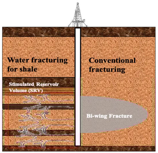
Figure 1.
Schematic diagram of different artificial fracture geometry for conventional fracturing and water fracturing.
Different from conventional fracturing, the goal for shale fracturing is breaking the formation and generating larger stimulated reservoir volume (SRV) with more complex fracture, due to the extremely low permeability and porosity of shale rock [3]. Therefore, the low viscosity water is used as the primary fracturing fluid system used for the stimulation of shale formation [4,5]. However, the low viscosity of the fluid affects the proppant transport capability. To address this problem, engineers often pump water–proppant mixture into the fracture at a very high pumping rate. Due to the low-viscosity fluid and high pumping rate, the turbulence effects become an important factor affecting the transport behaviors of the proppant particles in fracture [6,7]. In general, Reynolds number (Re) is a dimensionless number that can be used to characterize fluid flow type. For the general channel flow field, Re = 2000 is a critical value for laminar flow and turbulent flow, and we defined high Reynolds number condition (HRNCs) when Re is larger than 2000. The behavior and mechanism of the proppant transport process and placement under that HRNCs in the shale fracturing process are different from conventional fracturing. Because of its complexity and significance, continuous research on this problem is conducted by many scholars.
Numerous laboratory experimental research contributes to the understanding of the transport and settling behaviors in low viscosity fracturing fluids. The first experiment about the sand-water mixture transport in the slot is carried by Kern et al. [8], in which they found the sand quickly settled to the slot bottom and formed a proppant dune near the inlet side because of the poor sand-carrying ability of water. Besides, once the equilibrium height reached, sand injected later moved and settled to the rear of the proppant dune. STIM-LAB has been studied on the proppant transport process for more than 20 years, and the effects of the proppant density, diameter, and volume concentration on the equilibrium height of the proppant bed are comprehensively investigated [9,10]. Liu et al. [11] conducted similar slot experiments to STIM-LAB, and the results showed that the initial position and the equilibrium height of the proppant bed changed with the perforation position and the slurry flow rates. Palisch et al. [12] concluded that as the equilibrium height reached the critical value, the mechanisms of the proppant particles transporting on the top of the proppant dune were dominated by fluidization and sedimentation. The turbulent flow suspended the proppant particles off the proppant dune, and then proppant settled again after being transported to some distances during fluidization.
Based on the experimental results above, some correlations for the proppant particle transport and settling have been built up. Liu et al. [11] developed a fitting equation of the height of the equilibrium gap and the injection flow rate. Patankar et al. [9] and Wang et al. [13] established the empirical correlations in the form of power and bi-power law, which were widely used in the industry. Since there is no accurate method for the proppant particles settling in slick-water fracturing treatments, some revised Stokes’ Laws which considered the effects of the proppant volume concentration and the fracture wall are often used to predict the proppant particles settling [14,15].
Due to the ability to solve the flow patterns of liquid-solid two phases and their interaction simultaneously, Computational Fluid Dynamics (CFD) technology provides an alternative method to study the proppant transport and to settle in hydraulic fracture accurately. Patankar et al. [16,17] used a DNS model to study the lift-off of particles in plane Poiseuille flows. The results showed the interactions between the particles in the sedimentation process, ignoring the fracture propagation and the effect of fracturing fluid loss. Tsai et al. [18] employed a large-eddy model to simulate the flow field and tracked the proppant particles in Lagrangian coordinates, where the Wen-Yu drag model was used to couple the interaction of the fracturing fluid and proppant. The results showed that the pumping rate and the proppant parameters have an essential influence on the proppant settling and placement. A Computational Fluid Dynamics coupled with Discrete Element Method (CFD-DEM) was employed by Zeng et al. [6] to study the proppant transport process in a small-scale fracture. Although a representative particle model was used to reduce computational efforts, the time consumed is still considerable [19].
Compared with the CFD method mentioned above, the Eulerian multiphase flow model has the advantages of high efficiency and low computational cost. This method is the priority choice for the fluid–solid multiphase flow simulations of the engineering problems [20]. In the last three decades, the Eulerian multiphase flow model has gained considerable progress [21]. As described by Agrawal et al. [22], the solid phase governing equations was extended from the mono-disperse system to the poly-disperse system. Srivastava et al. [23] developed a solid phase frictional stress model in the dense solid-phase flow by considering the interactions between the particles as the solid volume concentration is greater than the critical concentration. Benyahia et al. [24] evaluated Jenkins-Louge and Johnson-Jackson’s solid wall boundary conditions and pointed out their application scope. The simulation results of the fluidized bed and the slurry flow in the pipeline using the Eulerian multiphase flow model were highly consistent with experimental results [25,26]. Recently, this method is also used to investigate the transport and settling behavior of proppant in single fractures [27] and the cross fractures [28].
Although Eulerian multiphase flow has been widely used in proppant transportation research, the systematic study of proppant transport mechanisms and behavior under HRNCs has not been reported before. In this paper, a Eulerian two-fluid model considering turbulence effect and particle friction stress were used to study the proppant transport and settling behaviors under HRNCs. The mechanism during the transport process under HRNCs and the impact of such factors as the inlet velocity, the inlet position, the proppant parameters, and the volume concentration on proppant transport and settlement are comprehensively discussed. The equilibrium height of the proppant dune was also studied, and a modified equilibrium height prediction model was proposed.
2. Eulerian Multiple Flow Model
2.1. Governing Equations
Based on kinetic theory, continuity and momentum equations were established for fluid and solid phase, respectively [21]. Continuity equation of the solid phase (m = s) and the fluid phase (m = l) is given by:
where and is the solid and liquid phase volume concentration, dimensionless; and is the density of solid and liquid phase, kg/m3; an is the velocity vector of solid and liquid phase, m/s.
Momentum equation for the fluid phase is given by:
Momentum equation for the solid phase is given by:
where and is the shear stress tensor of the fluid phase or solid phase, Pa; is the momentum exchange coefficient between two phases, dimensionless; and is the acceleration of gravity, m/s2.
The granular temperature for the solid phase represents the kinetic energy of the random motion of the solid particles [26]. The transport equation derived from the kinetic theory is taken as the following form:
where is the granular temperature, m2/s2; is the diffusion coefficient, kg/(m∙s); is the rate of the dissipation granular energy by inelastic collisions per unit volume, kg/(m∙s3); is the rate of the dissipation granular energy by inelastic collisions per unit volume, kg/(m∙s3).
In the artificial fracture, due to the low viscosity and high pumping rate, the flow state of the liquid phase may become turbulent flow. According to the research of Pfleger et al. [29], the predictions of the liquid phase turbulence kinetic energy k and its rate of dissipation are obtained from the following modified liquid phase turbulence model:
where k and is turbulence energy and its rate of dissipation, m2/s2 and m2/s3; is the turbulence viscosity coefficient and is the liquid molecular viscosity, Pa∙s, is the production term of the turbulence kinetic energy, kg/(m∙s3). According to Pfleger et al. [29], the source terms and are not considered yet. The constant parameters used in different equations are as follows: , , ,, .
2.2. Constitutive Equations
In the simulation presented here, the accumulation of high-concentration proppant in the proppant dune and the low-concentration on the dune appear at the same time. So, the drag correlation of Gidaspow et al. [30] was used due to the flexibility under different solid-phase concentrations:
where is the liquid volume fraction and the drag coefficient between phases is given by:
where is the particle diameter, m. is Reynolds number defined by the relative velocity between two phases:
The Reynolds stress tensor for the liquid phase is given by:
where is liquid phase effective viscosity, Pa∙s; is the turbulent viscosity, Pa∙s.
The stress tensor for the solid phase is given by:
where is the second-order identity tensor, dimensionless; s is the stress strain of solid phase, s−1; is the frictional pressure of the solid phase, Pa.
The strain stress for the solid phase is given by:
Solid kinetic-collisional pressure is given by:
where and is the particle-wall restitution coefficient, dimensionless.
The radial distribution function at contact is given by:
Solid-phase shear viscosity model is given by:
where is the granular viscosity with the effect of the interstitial fluid, Pa∙s; is the solids phase dilute granular viscosity, Pa∙s; and is the bulk viscosity of the solid phase, Pa∙s [22].
Granular energy conductivity coefficient is given by:
where is the granular conductivity with the effect of the interstitial fluid, and is the solid phase dilute granular conductivity, W/(m·K).
Considering the complexity between the particles in the proppant dune with high volume fraction, solid-phase frictional pressure and viscosity model [22] are given by:
where
where is the solid critical pressure, Pa; is the solid friction pressure, Pa. is the internal frictional angle of the solid phase; is the maximum packing concentration of the solid phase, and is the minimum frictional solid concentration, dimensionless.
The generation term of the turbulent kinetic energy is given by
Collisional dissipation term of the granular energy is given by
The interaction model of turbulence [31] is given by:
In this study, the parameters used in upper equations are set as: e , , , , , .
2.3. Boundary Conditions
The values of the liquid phase velocity the solid phase velocity , and the volume concentration were given as the inlet conditions. The pressure value of 0 Pa was set as the outlet conditions.
The nonslip condition was used for the liquid phase, and Johnson-Jackson model [20] was used for the solid phase.
The use of wall function allows the computation of turbulent flows without the need to resolve the turbulent boundary layer. The boundary layer for liquid phase [31] is defined as
The production and dissipation of as well as at the fluid cells adjacent to the wall, is given by:
where is a Constant in wall function formulation, 9.81; is Von Karmen constant of value, 0.42; is width of computational cell next to the wall, m.
2.4. Geometric Model and Solution Strategy
As shown in Figure 2, the length, width, and height of the slot were 4 m, 0.01 m, and 0.4 m, respectively. Three types of inlet positions of the top inlet, the middle inlet, and the bottom inlet were chosen to discuss the influence of the perforation positions in vertical hydraulic fractures. Eight outlets with a height of 0.02 m and a width of 0.01 m are uniformly distributed at the right wall.
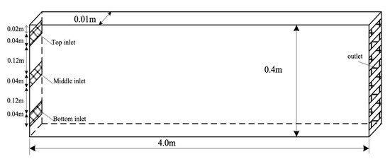
Figure 2.
Schematic diagram of slot geometry.
In order to verify the independence of the mesh, Figure 3 shows the proppant placement profile with different kinds of mesh conditions at T = 15 s. Obviously, mesh sizes will affect the final calculation results. But when the grid size is changed from to in the fracture length, height, and width directions, the proppant placement profile will no longer change. In order to obtain more detailed flow field information, we chose as our computing grid in this study.
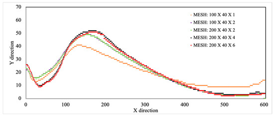
Figure 3.
Numerical simulation result of proppant placement profile under different mesh conditions at T = 15 s.
Multiphase solver MFIX was used for the simulation. MFIX (multiphase flow with interphase exchanges) is an open-source code used for multiphase computational fluid dynamics simulations that were developed at National Energy Technology Laboratory (NETL, Pittsburgh, United States) [14,21,24,26]. The governing equations were discretized with the finite volume method and solved on a staggered grid. A second-order super bee discretization scheme was used for all variables. The transient numerical solution was obtained within a residual tolerance of less than 10−4. It takes about 74 h to complete the calculation of a single working condition in 60 s, with i7-7700 cpu, calling 4 threads. The plane at the center along the slot width was used to display the simulation results.
3. Results and Discussions
3.1. Verification of Simulation on Proppant Transport
To verify the Eulerian two-phase simulation on proppant transport, the proppant transport experiments on laboratory scale were conducted. The experiment was conducted in a fracture with a length, width, and height of 4 × 0.006 × 0.6 m, which comprised two pieces of parallel transparent plexiglass (shown in Figure 4). The proppant-water mixture was injected into a slot from perforation to mimic an artificial fracture. The parameters for experiment and simulation were set as the same, and the average Reynolds number is 3000 for both cases. The specific details were shown in Table 1.
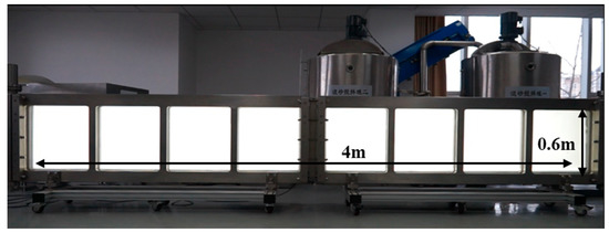
Figure 4.
Proppant transport experimental system.

Table 1.
Parameters set for experiment and simulation.
Figure 5 shows the comparison of the proppant placement structure between experiment and simulation in the whole transportation process. In the early stage, the experiment result showed the proppant settled near the entrance and formed two dunes (Figure 5a), which was coinciding with the simulation case (Figure 5e). As proppant continued to be injected, the proppant dune first grew vertically and then grew horizontally (Figure 5b,c), and these characteristics were also can be demonstrated through numerical simulation (Figure 5f,g). Finally, the whole process had reached the equilibrium state for experiment and simulation cases. The final placement of proppant obtained by numerical simulation was basically consistent with the experimental results (Figure 5d,h).
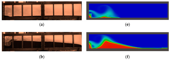
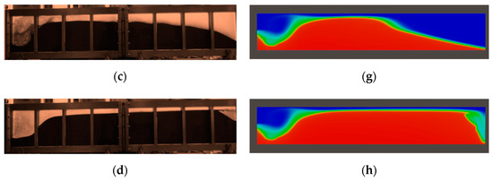
Figure 5.
Experimental and numerical simulation results of proppant transport and settlement process. (a–d): Proppant placement in the experiment process; (e–h): Corresponding proppant placement in the simulation process.
Specifically, Figure 6 shows the comparison of the proppant placement pattern obtained from the experiment and the simulation at the final equilibrium state. Due to the fracture height were different, the relative height was used to compare the equilibrium height in the experiment and simulation, which was defined as the height of the proppant bank to the fracture height. The background picture was obtained from the experiment result, while the white dot line was extracted from the proppant placement profile obtained from the simulation result. The result shows that the profile of the proppant bank for the simulation case is generally consistent with the experiment result, even though some small differences exist in the inlet and outlet place. The reason for this difference may be: (1). The proppant particle size used in the experiment is nonuniform (0.4–0.8 mm), while the proppant size for simulation is set as constant at 0.8 mm; (2). the fracture outlet in the experiment is a single outlet at the top of the wellbore, while six outlets were uniformly distributed along the wellbore in numerical simulations. Hence, the placement near the outlet of the two cases was slightly different from each other. Despite these differences, the Eulerian two-phase model can effectively simulate proppant dynamic behavior and static placement pattern under HRNCs, which proves that this model can be used to simulate and predict the proppant transport and settlement in the fracture.
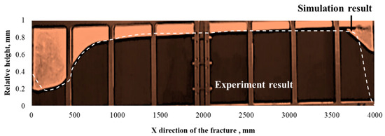
Figure 6.
Comparison of proppant placement pattern obtained from experiment and simulation at the final equilibrium state.
3.2. Proppant Transport Process
In this section, by choosing the same simulation parameters in Table 1, proppant transport characteristics and mechanisms under HRNCs were comprehensively studied by analyzing the solid phase velocity field. As we discussed above, the typical proppant transportation process was divided into four typical main stages; those are: Initial settlement stage, vertically grow stage, horizontally grow stage, and equilibrium state stage.
3.2.1. Stage1: Initial Settlement Stage
In the initial settlement stage, as the water–proppant mixture was injected form the middle inlet, two opposite vortexes were generated at the upper and lower ends of the slurry jet, and the lower one was smaller because of the inhibition generated by the slurry jet, as shown in Figure 7a. The injected proppant tended to quickly settle to the bottom and formed a proppant dune with a distance from the left boundary due to the gravity effect and the energy dissipation generated by the vortex. We defined this dune as the primary dune. Meanwhile, the small part of the proppant was dragged by the lower vortex move to the opposite direction and settle near the left boundary. We defined the small dune generated here as the secondary dune. Due to the slurry flush, a none proppant placement area was created between the two dunes. In this stage, this process was governed by the slurry vortex and the settlement.
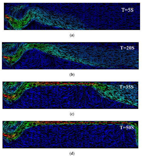
Figure 7.
Four stages for proppant transport under high Reynolds number condition. (a) initial settlement Stage; (b) vertically grow Stage; (c) horizontally grow Stage; (d) equilibrium State Stage.
3.2.2. Stage2: Vertically Grow Stage
Figure 7b shows the vertically grow stage. The flow region in the fracture was divided into three main regions; those are free clean fluid flow area in the upper side of the primary dune, transition flow area on the surface of the dune, and the immobile area beneath the surface. In this stage, the liquid phase velocity near the primary dune was too small to carry proppant to a distant place. Therefore, most of the injected particles settled quickly on the proppant dune, and only a small part of them was carried to the deep part of the fracture. With a continuous injection of slurry, more proppant settled on the primary and secondary dunes, and the flow path between the dune and fracture upper surface became narrower. Therefore, the fluid velocity became larger, which increased the fluidization of the settled particles and reduce the proppant settlement. Besides, the primary dune reached a specific height at 0.28 m and stopped growing vertically, and we defined the height as the primary equilibrium height (PEH). Additionally, the secondary dune grew gradually near the entrance. The lower vortex was getting weaker in this stage due to the collective effects caused by the boundary, secondary dune, and the inject slurry flow. Consequently, the lower vortex disappeared while the secondary dune stopped growing. The valley between the two dunes was still existed due to the flushing. In this stage, the proppant transport process was governed by the fluidization, settlement, and suspension.
3.2.3. Stage3: Horizontally Grow Stage
Figure 7c shows the proppant bank development process in a horizontal direction. In this process, because of the presence of the narrow gap between the proppant bank and the upper boundary, water had enough speed to fluidize and suspend the proppant. Therefore, a great amount of proppant transported through the currently generated proppant bank rather than retarded on the surface. However, once the proppant passes through the channel between the primary dune and wall, the velocity decreased dramatically because of the increased flow cross-section. Besides, another vortex was generated just behind the dune. Due to these two reasons, water cannot carry proppant into the deep of the fracture. Proppant gradually accumulated in the front of the formed proppant dune until reaching the equilibrium height, in which the water can suspend the proppant again. The settlement-reach equilibrium height process will repeat again and again, and from a macro perspective, the proppant dune will gradually grow horizontally. In this stage, the proppant distribution is determined by the settlement, fluidization and saltation.
3.2.4. Stage4: Equilibrium State Stage
As the proppant dune grew horizontally and reached the outlet boundary, the proppant dune remained unchanged and reached a comprehensive equilibrium height (CEH), as shown in Figure 7d. The CEH was defined as the average equilibrium height of the primary dune when the proppant bank was stable during the injection process. The suspension and saltation were the main mechanisms to control the transport.
Figure 8 shows the proppant dune growth trajectory from 5 s to 65 s, in which the characteristic of the four main stages during the injection can be obviously obtained. Once the primary dune was formed, the dune will gradually grow vertically, and the front settlement angel almost remains constant at 20° until reaching the primary equilibrium height (PEH) by the end of the second stage (at around T = 20 s). The third stage began at T = 25 s, in which the proppant mainly grows horizontally, and the settlement angle of the upper side becomes more steep form 40° to nearly 90°. At T = 60 s, the proppant dune reaches the CEH.
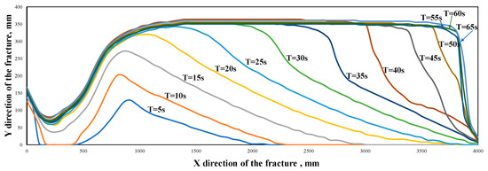
Figure 8.
Proppant dune growth trajectory from for the simulation of the control sample.
3.3. Parametric Study
In this section, the parametric study for different injection velocity, inject position, particle diameter, density, and concentration were conducted for a better understanding of the effects caused by these parameters on the proppant transport process under HRNCs. The parameter sets are listed in Table 2. The bold items are set as the control sample in the parametric study. In each section, besides the investigated parameter, other parameters were set as same as the control sample.
Table 2.
Parameter sets for parametric study and primary data for simulation.
3.3.1. Inlet Velocity Effect
Figure 9 shows the distribution of the liquid volume concentration during the transport process for different injection velocity. In this study, the injection velocity of fluid and proppant was set to be the same, and the velocity uniformly expressed as v. The parameters except velocity were set as the same as the control sample. The average Reynolds number are 2000–5000 for v = 2–5 m/s, respectively. Compared with the control sample, the lower velocity case for v = 2 m/s (Figure 9A) showed a closer distance from the primary dune to the entrance and more particle placement between the dunes, which was mainly because the vortex is weaker than that of the control sample. Meanwhile, the proppant dune grew rate for v = 2 m/s is a little bit slower than that of the control sample. On the contrary, as the injection velocity became faster, the vortex generated near the entrance became larger and stronger, resulting in a larger distance for primary dunes and disappeared secondary dune. As the velocity of the slurry increases from 2 m/s to 5 m/s, the non-propped area near the inlet increase by 5.3 times.
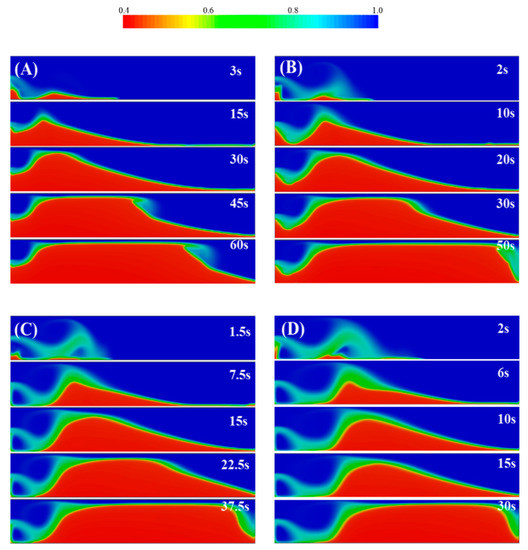
Figure 9.
Volume concentration of liquid phase during the transport process for different injection velocity cases: (A) v = 2 m/s, (B) v = 3 m/s, (C) v = 4 m/s, and (D) v = 5 m/s.
The efficiency of proppant placement is also an essential factor in evaluating the effect of proppant placement. Therefore, we defined the proppant occupation as a stationary proppant bed area over the total fracture area. The proppant occupation in equilibrium stages was defined as equilibrium proppant occupation (EPO), which indicated the maximum proppant accumulation in the fracture under the specific condition. Proppant occupation, together with the EPO and CEH, were used to characterize the proppant transport and settlement for each case.
Figure 10 shows the proppant occupation of different time steps and comparison of equilibrium height for different injection velocity cases. The case for v = 5 m/s reached the equilibrium stage at T = 22 s, which was the fastest among all instances. As velocity decreased, it takes longer for the proppant dune to reach equilibrium in the fracture. However, the v = 2 m/s cases yielded the highest CEH at 35.9 cm, compared with other cases, which were at 35.2 cm, 34.6 cm, and 34.1 cm, respectively. For the low-velocity instance, the gap between the primary dune needed to be narrower to obtain enough speed to balance the amount of settled and rolled-up proppant, resulting in higher CEH. Besides, due to the smaller (none) secondary dunes and the relatively shorter primary dune, it was observed that the EPO for large velocity is lower than those of slower cases during the transportation process, which are 80.5%, 74.6%, 66.4%, and 56.5% for the velocity from 2 to 5 m/s. The small EPO, especially caused by the no proppant placement neat the entrance, will cause worse conductivity in artificial fracture, which should be avoided in the field fracturing design.
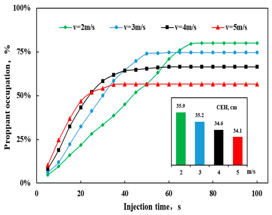
Figure 10.
Proppant occupation percentage in fracture change with time a comprehensive equilibrium height (CEH) for different velocity cases.
3.3.2. Effects of Inlet Position
Figure 11 shows the distribution of the proppant placement in the transport process under different inlet positions. According to Figure 11A, when the slurry was injected from the bottom, the distance between the initial settlement location and left wall was 1.1 m, which indicated that the flow velocity at this position was not able to overcome the frictional force between the proppant particles and the bottom wall. Since no flow vortex was formed upon the bottom wall, no proppant particles were situated in the region near the left wall. As a result, only the primary dune was generated in the fracture. Proppant particles injected later would get over the dune and settle at the rear of the dune. Finally, the proppant dune gradually grew until it reached the CEH.
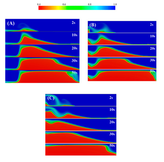
Figure 11.
Proppant placement during the transport process for different inlet position cases: (A) Inject from the bottom inlet; (B) inject from the middle inlet; and (C) inject from the top inlet.
Figure 11C shows the proppant transport process of the top inlet condition at different time points. When the mixture was injected into the slot, the proppant quickly settled to the bottom at the position about 0.65 m from the left wall. A big clockwise vortex was generated near the entrance and brought proppant back to the inlet side, forming a sizeable secondary dune. As the proppant was injected continuously, the heights of both dunes increase, and the trough between two dunes gradually filled with the proppant. Consequently, the primary and secondary dunes gradually became an integrated dune, and the CEH was obtained almost alone the whole length of the fracture.
According to Figure 12, it took almost the same time (55 s) to reach CEH for the three cases with different inlet positions. Injecting proppant from the top could produce the highest equilibrium height at 36.1 cm, compared with that of the middle case at 35.2 cm and the bottom situation at 34.3 cm. Besides, the proppant occupation curve indicated that the proppant injected through the top yielded the highest proppant placement percentage, and the EPO reaches 82.3% compared with the middle case at 74.6% and the bottom case at 67.8%. The result identified that the vortex at the front end of the fracture is the dominant factor for proppant placement near the entrance. The large vortex could carry the proppant back to the inlet place. The large non-propped area in the fracture may cause fracture closure after pumping, resulting in the permeability significantly decreased. Therefore, choosing the relatively high inlet positions will result in better patterns of the proppant placement and improve fracture conductivity.
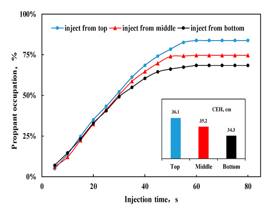
Figure 12.
The curve for proppant occupation percentage in fracture change with time and CEH for different inlet position cases.
3.3.3. Effects of Particle Diameter
Figure 13 shows the effects of particle diameter on transport processes. The accumulation curve demonstrated that the larger particles settle more in the fracture at any time during the transport process because smaller particles were easier carried by the fluid. The smaller particle was carried into the far end of the fracture rather than accumulated during the transportation. For the same reason, it took a long time for smaller particles to reach CEH. However, the CEH difference is tiny among different cases, which indicated the proppant diameters had little effect on the primary dune for a relatively long time in the transport process. At last, EPO for 1 mm to 0.6 mm are 67.6%, 68.8%, 71.0%, 73.1%, and 74.6% respectively.
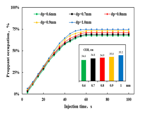
Figure 13.
The curve for proppant occupation percentage in fracture change with time and comprehensive equilibrium H = height (CEH) for different particle diameter cases.
3.3.4. Effects of Particle Density
Figure 14 shows the detailed data extracted from the simulation results for different particle density. The results indicated proppant density has a significant influence on the proppant settlement in the fracture. The curve shows that the lighter particle has the least amount of settlement in the fracture during the injection process. The reason for that phenomenon was that the lighter particles were more likely to be fluidized and dragged by the fluid to the further side of the fracture. All the cases almost reached the equilibrium height at the same time, around 45 s. The EPO was 60.39% when the density was 1800 kg/m3 is, which was 21.3% smaller than that of 3200 kg/m3. For the CEH study, it was interesting to obtain a proppant density threshold for the particle dune growth. When the density is small, the equilibrium height increases rapidly as the proppant density increases, which changed from 32.8 cm in the 1800 kg/m3 case to 35.8 cm in the 2500 kg/m3 case. However, when the density was larger than 2500 kg/m3, the CEH almost unchanged.
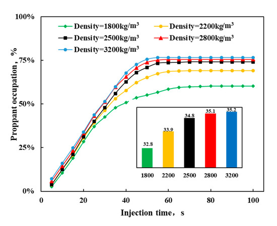
Figure 14.
The curve for proppant occupation percentage in fracture change with time and CEH for different inlet particle density.
3.3.5. Effects of Solid-Phase Volume Concentration
Figure 15 shows the particle concentration effects on proppant transport. From the curves, higher proppant concentration resulted in a greater amount of settlement in the fracture at the same time. Besides, the lowest concentration (10%) case was the last one to reach the CEH at T = 76 s, which almost double that of 25% concentration This phenomenon was caused by two reasons; those are fewer injection particle amounts and easy fluidization for proppant when the concentration was low. Moreover, the CEH for lower concentration cases was also shorter, which may result from more liquid fluid flowing past over the top of the proppant bed or the higher ability of lower solid phase volume concentration to fluidize the proppant particles. In conclude, the lower concentration in the transport process lead to a more proppant place in the further part of the fracture, which was good for longer effective propped fractures. However, less proppant in the fracture may result in poor conductivity. The proppant particle concentration selection in the field should be considered comprehensively for both sides.
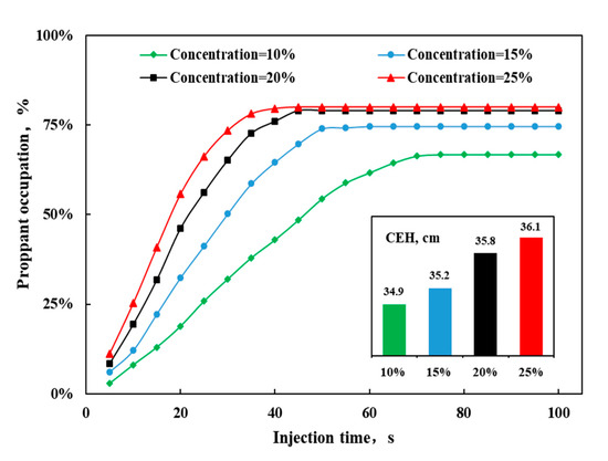
Figure 15.
The curve for proppant occupation percentage in fracture change with time and CEH for different inlet position cases.
3.4. Equilibrium Height Prediction Model
The height of the equilibrium gap H, which was defined as the distance between the top of the proppant bed and the upper wall boundary, was used to represent the equilibrium height. J. Wang et al. [13] established a Bi-power law correlation for the equilibrium gap of the proppant bed, and it was given by:
The gravity Reynolds number RG is defined as:
The gravity Reynolds number for the fluid is defined as:
The fluid Reynolds number Rf is shown as:
The proppant Reynolds number Rp is defined as:
where H1 is the height of equilibrium gap, ml; W is the fracture width, m; is gap height over fracture width, dimensionless;
Along the altitude direction of the fracture, the flow field can be divided into three layers. The bottom of the proppant bank is an immobile layer in which the velocity of the proppant particles is approaching zero. The middle layer is a mobile zone that is above the stationary bed, in which the proppant particles move by sliding and rolling or a combination of both. The top layer is a clean liquid zone. As the proppant concentration increases gradually from the fresh liquid layer to the mobile layer and then to the immobile layer, the point with the proppant concentration equal to 0.5 was chosen to be the top of the stationary bed.
Figure 16 shows the comparison of dune height between the simulation result and Wang’s model under different conditions. As the parameters change, they had the same trend. However, compared with Wang’s model, the equilibrium height obtained by the simulation was always higher. The mean deviation for the case of density, diameter, velocity, and solid concentration was 45.8%, 36.5%, 57.7%, and 59.4%, respectively, which indicated it is difficult to accurately predict the equilibrium height by using this model.
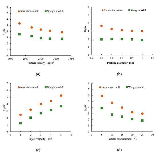
Figure 16.
Comparison of the equilibrium dune height between simulation result and Wang’s model. (a): Comparison of particle density; (b) comparison of particle diameters; (c) comparison of injection velocity; and (d) comparison of particle concentration.
In this paper, some modification about Wang’s model was conducted based on the simulation result, to accurately predict the equilibrium height of the proppant dune in the fracture under HRNCs. The new prediction model is shown as:
Figure 17 shows the relationship between the new prediction model and simulation results. It can be seen from the comparison that this prediction model can fit the simulation result very well. Through calculation, the mean deviation is only 3.8%. The applicable range for this prediction model is the case where the Reynolds number is 2000–5000. This correlation can be used to quickly predict proppant placement in a fracturing simulator, which can greatly improve the simulation accuracy.
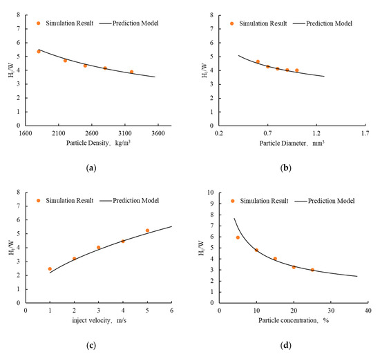
Figure 17.
Comparison of the equilibrium dune height between simulation result and new prediction model. (a) Comparison of particle density; (b) comparison of particle diameters; (c) comparison of injection velocity; and (d) comparison of particle concentration.
4. Conclusions
In this work, a Eulerian two phases model is used to simulate the proppant transport process in low viscosity fluid and high-speed rate conditions (HRNCs). The turbulence effect and particle-particle/wall effect are the primary concern in this paper. According to the comparison of the results of the numerical simulations and the experimental study, the Eulerian multiphase model can capture the transport and settling behaviors of proppant in the water fracture treatments. Based on the simulation results, the following conclusions have been drawn on:
- (1)
- The transport process can be classified into four main stages. In addition to the mechanisms such as fluidization, suspension, and settlement presented by other studies, the vortex is also a critical mechanism in the transport process under HRNCs, especially near the entrance.
- (2)
- The inlet positions significantly influence the vortex and the proppant placement patterns. There is a nearly non-propped zone near the wellbore for the bottom inlet condition since no reversed flow is generated to take the proppant particles back. Higher inlet position increases the propped area near the wellbore by 7.1 times. But the blocking of the entrance may lead to high risk in pumping proppant.
- (3)
- Increasing the injection velocity from 2 m/s to 5 m/s, the proppant particles easier to be fluidized and increase the distance to which the proppant particles are transported in the hydraulic fracture. The non-propped area near the inlet increase by 5.3 times and the equilibrium height decrease by 5.2%.
- (4)
- A new prediction model is proposed to predict the equilibrium height of the proppant bank in the fracture under high Reynolds number condition. Compared with the simulated data, the mean deviation between them is only 3.8%, which indicates the model is suitable under HRNCs (2000–5000).
Author Contributions
Conceptualization, T.Z. and J.G.; Data curation, R.Y.; Formal analysis, R.Y. and J.Z.; Investigation, J.G.; Methodology, T.Z.; Project administration, J.G.; Supervision, T.Z.; Validation, T.Z.; Writing—original draft, R.Y.; Writing—review and editing, J.G. and J.Z. All authors have read and agreed to the published version of the manuscript.
Funding
This study was supported by the National Science and Technology Major Project (2016ZX05048-004-006), National Science and Technology Major Project (2016ZX05002-002), and the National Science Fund for Distinguished Young People (51525404).
Conflicts of Interest
The authors declare no conflict of interest.
References
- Palisch, T.T.; Vincent, M.C.; Handren, P.J. Slickwater fracturing: Food for thought. In Proceedings of the SPE Annual Technical Conference and Exhibition, Denver, CO, USA, 21–24 September 2008. [Google Scholar]
- King, G.E. Thirty Years of Gas Shale Fracturing: What Have We Learned? In Proceedings of the SPE Annual Technical Conference and Exhibition, Florence, Italy, 20–22 September 2010. [Google Scholar]
- Handren, P.; Pslish, T. Successful Hybrid Slickwater-Fracture Design Evolution: An East Texas Cotton Valley Taylor Case History. SPE Prod. Oper. 2009, 24, 415–423. [Google Scholar] [CrossRef]
- Guo, J.; Li, Y.; Wang, S. Adsorption damage and control measures of slick-water fracturing fluid in shale reservoirs. Pet. Explor. Dev. 2018, 45, 336–342. [Google Scholar] [CrossRef]
- Sahai, R. Laboratory Evaluation of Proppant Transport in Complex Fracture Systems. Ph.D. Thesis, Colorado School of Mines, Arthur Lakes Library, Golden, CO, USA, 2012. [Google Scholar]
- Zeng, J.; Li, H.; Zhang, D. Numerical simulation of proppant transport in hydraulic fracture with the upscaling CFD-DEM method. J. Nat. Gas Sci. Eng. 2016, 33, 264–277. [Google Scholar] [CrossRef]
- Britt, L.K.; Smith, M.B.; Haddad, Z.A.; Lawrence, J.P.; Chipperfield, S.T.; Hellman, T.J. Waterfracs: We Do Need Proppant After All. In Proceedings of the SPE Annual Technical Conference and Exhibition, Antonio, TX, USA, 24–27 September 2006. [Google Scholar]
- Kern, L.R.; Perkins, T.K.; Wyant, R.E. The mechanics of sand movement in fracturing. J. Pet. Technol. 1959, 11, 55–57. [Google Scholar] [CrossRef]
- Patankar, N.A.; Joseph, D.D.; Wang, J.; Barree, R.D.; Conway, M.; Asadi, M. Power law correlations for sediment transport in pressure driven channel flows. Int. J. Multiph. Flow. 2002, 28, 1269–1292. [Google Scholar] [CrossRef]
- Wookworth, T.R.; Miskimins, J.L. Extrapolation of laboratory proppant placement behavior to the field in slickwater fracturing application. In Proceedings of the SPE Hydraulic Fracturing Technology Conference, College Station, TX, USA, 29–31 January 2007. [Google Scholar]
- Liu, Y. Settling and Hydrodynamic Retardation of Proppants in Hydraulic Fractures. Ph.D. Thesis, The University of Texas, Austin, TX, USA, 2006. [Google Scholar]
- Palisch, T.T.; Vincent, M.; Handren, P.J. Slickwater fracturing: Food for thought. SPE Prod. Oper. 2010, 25, 327–344. [Google Scholar] [CrossRef]
- Wang, J.; Joseph, D.D.; Patankar, N.A.; Conway, M.; Barree, R.D. Bi-power law correlations for sediment transport in pressure driven channel flows. Int. J. Multiph. Flow 2003, 29, 475–494. [Google Scholar] [CrossRef]
- Barree, R.D.; Conway, M.W. Experimental and numerical modeling of convective proppant transport. In Proceedings of the SPE Annual Technical Conference and Exhibition, New Orleans, LA, USA, 25–28 September 1994. [Google Scholar]
- Warpinski, N.R.; Mayerhofer, M.J.; Vincent, M.C.; Cipolla, C.L.; Lolon, E.P. Stimulating unconventional reservoirs: Maximizing network growth while optimizing fracture conductivity. J. Can. Pet. Technol. 2009, 48, 39–51. [Google Scholar] [CrossRef]
- Patankar, N.A.; Huang, P.Y.; Ko, T.; Joseph, D.D. Lift-off of a single particle in Newtonian and viscoelastic fluids by direct numerical simulation. J. Fluid Mech. 2001, 438, 67–100. [Google Scholar] [CrossRef]
- Patankar, N.A.; Ko, T.; Choi, H.G.; Joseph, D.D. A correlation for the lift-off of many particles in plan Poiseuille of Newtonian fluids. J. Fluid Mech. 2001, 445, 55–76. [Google Scholar] [CrossRef]
- Tsai, K.; Fonseca, E.; Lake, E.; Degaleesan, S. Advanced Computational Modeling of Proppant Settling in Water Fractures for Shale Gas Production. SPE J. 2012, 18, 1389–1394. [Google Scholar]
- Zhou, Z.Y.; Pinson, D.; Zou, R.P.; Yu, A.B. Discrete particle simulation of gas fluidization of ellipsoidal particles. Chem. Eng. Sci. 2011, 66, 6128–6145. [Google Scholar] [CrossRef]
- Benyahia, S.; Syamlal, M.; O’Brien, T.J. Evaluation of boundary conditions used to model dilute, turbulent gas/solids flows in a pipe. Powder Technol. 2005, 156, 62–72. [Google Scholar] [CrossRef]
- Pannala, S.; Syamal, M.; O’Brien, T.J. Computational Gas-Solids Flows and Reacting Systems: Theory, Methods and Practice; IGI Global: Hershey, PA, USA, 2010. [Google Scholar]
- Agrawal, K.; Loezos, P.N.; Syamlal, M. The role of meso-scale structures in rapid gas-solid flows. J. Fluid Mech. 2001, 445, 151–185. [Google Scholar] [CrossRef]
- Srivastava, A.; Sundaresan, S. Analysis of a frictional–kinetic model for gas–particle flow. Powder Technol. 2003, 129, 72–85. [Google Scholar] [CrossRef]
- Benyahia, S. Analysis of Model Parameters Affecting the Pressure Profile in a Circulating Fluidized Bed. AIChE J. 2012, 58, 427–439. [Google Scholar] [CrossRef]
- Kaushal, D.R.; Thinglas, T.; Tomita, Y.; Kuchii, S.; Tsukamoto, H. CFD modeling for pipeline flow of fine particles at high concentration. Int. J. Multiph. Flow. 2012, 43, 85–100. [Google Scholar] [CrossRef]
- Benyahia, S. On the effect of subgrid drag closures. Ind. Eng. Chem. Res. 2010, 49, 5122–5131. [Google Scholar] [CrossRef]
- Zhang, T.; Guo, J.C.; Liu, W. CFD Modeling of Proppant Transport and Settling in Water Fracture Treatments. J. Southwest Pet. Univ. 2014, 36, 74–82. [Google Scholar]
- Li, P.; Zhang, X.; Lu, X. Numerical simulation on solid-liquid two-phase flow in cross fractures. Chem. Eng. Sci. 2018, 181, 1–18. [Google Scholar] [CrossRef]
- Pfleger, D.; Gomes, S.; Gilbert, N.; Wagner, H.G. Hydrodynamic simulations of laboratory scale bubble columns fundamental studies of the Eulerian-Eulerian modelling approach. Chem. Eng. Sci. 1999, 54, 5091–5099. [Google Scholar] [CrossRef]
- Gidaspow, D.; Bezburuah, R.; Ding, J. Hydrodynamics of Circulating Fluidized Beds, Kinetic Theory Approach. In Proceedings of the 7th Engineering Foundation Conference on Fluidization, Brisbane, Australia, 3–8 May 1992; pp. 75–82. [Google Scholar]
- Benyahia, S.; Syamlal, M.; O’Brien, T.J. Study of the Ability of Multiphase Continuum models to predict core-annulus flow. AICHE 2007, 53, 2549–2568. [Google Scholar] [CrossRef]


Publisher’s Note: MDPI stays neutral with regard to jurisdictional claims in published maps and institutional affiliations. |
© 2020 by the authors. Licensee MDPI, Basel, Switzerland. This article is an open access article distributed under the terms and conditions of the Creative Commons Attribution (CC BY) license (http://creativecommons.org/licenses/by/4.0/).