Non-Intrusive Load Monitoring via Deep Learning Based User Model and Appliance Group Model

Abstract

Non-Intrusive Load Monitoring (NILM) increases awareness on user energy usage patterns. In this paper, an efficient and highly accurate NILM method is proposed featuring condensed representation, super-state and fusion of two deep learning based models. Condensed representation helps the two models perform more efficiently and preserve longer-term information, while super-state helps the model to learn correlations between appliances. The first model is a deep user model that learns user appliances usage patterns to predict the next appliance usage behavior based on past behaviors by capturing the dynamics of user behaviors history and appliances usage habits. The second model is a deep appliance group model that learns the characteristics of appliances with temporal and electrical information. These two models are then fused to perform NILM. The case study based on REFIT datasets demonstrates that the proposed NILM method outperforms two state-of-the-art benchmark methods.

1. Introduction

Buildings consume more than 76% electricity in the United States, which can be reduced up to 15–40% using a home energy management system (HEMS) [1]. The HEMS can make more intelligent decisions to cut energy bills and help users participate in demand response (DR) programs including renewable energy resources integration, frequency regulation, and so forth [2]. In order to realize a more effective HEMS that considers both users’ comfort preference and appliances’ operation flexibility [2], the HEMS must be provided with detailed energy consumption information. Non-Intrusive Load Monitoring (NILM) is a cost-effective approach to provide such detailed energy consumption of individual appliances based on only the aggregated power measured by a single upstream power meter. Generally, NILM requires appliance-level electricity consumption to learn a machine learning model in learning phase, and the down-stream sensors are removed during operation [3,4,5,6,7,8,9,10].

1.1. Feature Sets for NILM

Some NILM methods use data of high sampling rates (>1 kHz) to obtain more distinguishable features and achieve better performance by applying Fourier analysis [11], discrete wavelet transforms [12] and using such features as V-I trajectory [13] and harmonic information. However, in most household applications of NILM, only power readings with low sampling rates can be obtained due to communication bandwidth and measurement hardware cost constraints [2]. Hence, in this work, we focus on NILM with sampling rates of 1/60 Hz or lower.

By utilizing more electrical information such as reactive power [14], power phase angle, and power factor, the performance of NILM could be improved. However, in most cases only active power information is available, which is typical in the case of smart meters [2]. For these time series of active power readings, trajectory is a common choice to distinguish different appliances, and dynamic time wrapping (DTW) based algorithm is applied to measure the difference in trajectories [9,15]. DTW does not need time series to be of equal length, nor does it require scaling the time series shapes to zero mean and unit standard deviation, which is important in NILM because the amplitude of time series may contain valuable information [9]. Researchers also found that introducing the difference in aggregated power between consecutive time slices could lead to improvement in NILM performance, and the differential observations are generally combined with amplitude, trajectories, and so forth, and fed into a machine learning model to perform NILM [16,17].

The performance of NILM could also be enhanced by introducing features out of the time-domain. To get these features, Discrete Wavelet Transform (DWT) [12], Karhunen Loéve Expansion (KLE) [7], Bandt-Pompe method [18] are common choices. in these methods, a sliding window is required to extract features of the time series, used alone or combined with time-domain features.

Appliances also exhibit temporal usage patterns like time of day (TOD), on duration (OD), daily schedule of the users, switching-time (ST), and so forth [7,19]. Zhai et al. [2] showed that temporal usage patterns are related to user-behavior, which could be important in appliance monitoring. For example, lights are unlikely to be turned on during the day, and OD is important in detecting motors, whose working duration is likely to be relatively short [8]. Kim et al. [19] extended factorial HMM (FHMM) to consider additional temporal usage patterns, and Liu et al. [8] enhanced their probabilistic load detection approach to detect groups of appliances by considering OD, ST, and so forth.

1.2. Algorithms for NILM

The features above are fed into a machine learning model to perform NILM, and the model could be support vector machines [20], neural networks [21], k-nearest neighbor classifier [9], and decision trees [22].

Recent works have paid more attention on the dynamics of time series to perform NILM. Hidden Markov Model (HMM) based methods are the most popular for modeling dynamics on time series. The observation in HMM usually refers to power readings or differential power readings, while the hidden states may represent one or a group of appliances. in References [14,23], FHMM has been used for NILM, which contains several independent Markov chains evolving in parallel. Each appliance could be modeled as a single Markov chain in FHMM, and the observation is a joint function of all appliances [23]. FHMM captures the dynamics of individual appliances but the correlation of appliances usage patterns is lost, and the time complexity is too high to make exact inference [3]. Kong et al. [6] simplified the original formulation and relaxed the FHMM to a segmented integer quadratic constraint programming (SIQCP) problem. With the simplification, the computational efficiency as well as the performance of NILM is improved.

In order to integrate correlations between appliances into HMM, Makonin et al. [3] introduced super-state. Each super-state is a unique combination of appliance states, representing how a group of appliances works; hence in each time interval, the aggregated power to be disaggregated is represented by a single super-state. Then, the super-state HMM is built with each hidden state in conventional HMM is replaced by super-state. in doing so, HMM takes the dependencies between super-state into consideration, and the correlations between appliances are also preserved. super-state HMM has achieved the best performance by far, and the computational efficiency is also significantly enhanced, which makes it practical to run in real-time even on an embedded processor. Inspired by the idea of encoding correlations between appliances, this work adopts the concept of super-state in designing the relevant models.

The hidden states in HMM based NILM approaches are related through a Markov process, hence the probability of the appliances’ status at the current time is dependent only on their status at the previous time, ignoring higher higher-order dependencies. Status of appliances is statistically dependent on their status prior to many time intervals. Tabatabaei [12] considered higher-order dependencies between samples by encoding a number of past observations into delay embedding, which is a vector containing information about the past. the embedding is concatenated with current observation to predict the next one.

1.3. Influencing Factors of NILM

Data sampling rate: Sampling period of smart meters is usually 15 to 60 min, while the feature sets in Section 1.1 requires sampling rate to be 1/60 Hz or even higher.

Algorithm complexity: If high sampling rate data is used, fast Fourier transform and other methods can be used to extract features in short time. However, if the medium and low sampling rate data are used, the time and space complexity of algorithms such as HMM is relatively high [24], which can not be adopted to the situation of large number of appliances. For other algorithms such as KNN [2] and template matching [25], the model will become larger when the accuracy of the algorithm is improved (for example, the number of templates increases or the number of samples in KNN increases), resulting in slower algorithm efficiency.

Generalization capability: Generalization is the ability to recognize unseen appliances in the training set. the poor generalization capability of the NILM algorithm is mainly because the training data and the data collected during operation may follow different distributions, but if the model capacity is small, even if the training data distribution is the same as the real distribution and the amount of data is large enough, the model may still have poor generalization performance. For example, most HMM models assume that the power consumption of appliances follows a normal distribution, but in fact, the power of different appliances may be quite different, and the diversity of the same type of appliances cannot be considered by a single normal distribution. in order to enhance the generalization capability, the NILM algorithm should also consider its model capacity. One of the most effective work to improve the generation capability is transfer learning. in Reference [26], a deep learning model is trained to perform NILM at user A, and applying it to user B. If user B is similar to user A, we can use the model trained in user A as a initial model, then collect a small amount of labeled data from user B, and fine-tune it to perform NILM at the new user.

Lack of training data: NILM usually adopts supervised learning algorithm, which requires a large number of labeled data in the training stage, but the cost of obtaining the labeled data of NILM is very high. in many works, NILM algorithms can achieve high accuracy, but the results are obtained on the premise of sufficient labeled data. in Reference [19], the model are trained using the unsupervised EM algorithm [27], but its performance is greatly affected by initialization. in Reference [9], a semi-supervised learning approach is adopted, in which a small amount of labeled data is used to assign pseudo labels to some unlabeled data by measuring the Mahalanobis distance, expanding the labeled dataset. Then use the supervised learning method to perform load monitoring on the new labeled dataset.

1.4. Contributions

Compared with state-of-the-art works in the literature of NILM, the proposed NILM method in this paper has a higher computational efficiency, and better performance in steady-power appliances recognition. This is achieved by condensed representation and fusion of two deep learning based models.

Firstly, sequence of power readings is preprocessed by event detection [9], and inspired by Reference [28], the time series is condensed represented as sequence of $bin$s to reduce both sequence length and processing complexity.

Then, the $bin$s are fed into the appliance group model and the user model to perform NILM. The user model and the appliance group model are built separately with Deep Neural Network (DNN), which allows the model to consider multiple feature types while capturing long-term dependencies. DNNs are well known for their capability of modeling complex non-linear relationships and long-term dependencies, and have been successfully applied to fields including computer vision, speech recognition, and natural language processing. The user model is a detailed description of the user’s appliance usage patterns, namely, appliance usage dependency and temporal usage behaviors. the user model uses DNN to embed temporal information and encode user behavior history preserving higher-order dependencies, and predicts the user’s behavior. The appliance group model is represented by another DNN as a joint function of TOD, OD, power, and differential power. It can predict the probability of each appliance state based on the information in the current time interval. The user model and the appliance group model are then combined to predict the probability of each appliance state. Hence the proposed method preserves correlations between appliances as well as higher-order dependencies between appliance usage behaviors, and considers active power, differential power, temporal information, and so forth, to achieve better performance than those of the state-of-the-art methods.

2. NILM Problem Formulation

This work focuses on NILM with active power readings of low sampling rates (≤1/60 Hz). However, the proposed method can also work with additional features such as reactive power or with data of high sampling rates. In learning phase, up-stream meter data is condensed represented as the input of the models. Condensed representation can represent time series of power readings more efficiently, which can help retain information about longer context. Then, appliance states are extracted from sub-meters data, and these states are combined to create super-state, namely the target of the models. the NILM problem is reformulated into a sequence-to-symbols problem, in which the super-state in each time interval is the symbol to be inferred from sequence of condensed representations. In testing phase, sub-meters are removed and only up-stream meter is used to perform NILM.

2.1. Condensed Representation

Time series of power readings are generally sparse because appliances rarely change their states in short time scales (see Figure 1), and most appliances work with steady power consumption.

In this work, the time series of power readings are represented as sequence of $bin$s, which considers both temporal information and power consumption.

$$bins=[bi{n}_1,bi{n}_2,\dots ,bi{n}_{T-1},bi{n}_T].$$

(1)

Firstly, an event detection technique is applied to look for boundaries of $bin$s. We adopt an event detection scheme in Reference [9], where a differential observation bigger than a threshold $\theta$ is considered as an event. Then, each sub-sequence between a pair of adjacent events is represented as a $bin$:

$$\begin{array}{c}\hfill bi{n}_i=\{start\text{\_}time,delta\text{\_}time,mean\text{\_}power,delta\text{\_}power\},\\ \hfill i\in \{1,\dots ,T\},\end{array}$$

(2)

where $start\text{\_}time$, $delta\text{\_}time$, $mean\text{\_}power$ represent TOD, OD of the $bin$, and the mean power in the given sequence, respectively. $delta\text{\_}power$ is the power change between the beginning of the current $bin$ and the end of the previous $bin$.

In the literature on NILM, except for less memory usage, condensed representation could have other benefits because the computational complexity is significantly reduced and longer-term dependencies could be captured with the same model. For example, in Figure 1, compared with using the raw sequence of about 100 samples, it is much more efficient and easier to capture the dynamics and make inference of only 8 $bin$s for the same sequence of power readings.

2.2. Super-State

Super-state is firstly introduced by Makonin et al. [3], which is defined as the Cartesian product of the different possible states of each appliance. However, each appliance may have multiple states, for example, a washing machine has three on-states: wash, rinse, and spin [30]. Even in a house with a small number of appliances, the number of super-state is still large, because it grows exponentially as the number of appliance states increases. In this work, the idea of super-state is also adopted. But the appliances are divided into categories. Each category has two states—ON/OFF, hence the super-state is the Cartesian product of the different appliance category states. By doing so, the number of super-states is significantly reduced, In the REFIT dataset, there are 19 different appliances corresponding to 8 categories and $2^8=256$ super-states. Even though the number of super-states grows exponentially as the number of categories increases, the categories of household appliances in different houses are relatively fixed. Each super-state is encoded as one-hot vector to work with DNN.

Each subsequence between two adjacent events in Section 2.1 is assigned a particular super-state. As the event detection may not be accurate, some subsequences may correspond to multiple super-states. in this case, the subsequence is assigned the super-state with the highest frequency in the subsequence.

2.3. Electricity Consumption Estimation

So far, we have defined the input and target of the NILM problem. The input raw energy consumption data is firstly preprocessed to form a sequence of $bin$s with each entry having 4 channels. the target is another sequence with each element being a one-hot vector representing a particular super-state:

$$\begin{array}{c}\hfill target=[targe{t}_1,targe{t}_2,\dots ,targe{t}_T],\\ \hfill targe{t}_i\in \{super\text{\_}stat{e}_1,super\text{\_}stat{e}_2,\dots ,super\text{\_}stat{e}_K\}.\end{array}$$

(3)

The estimated total power at time t is the sum of the estimated appliance-level consumptions:

$${\widehat{y}}_t=\sum _{m=1}^M{\widehat{y}}_t^{\left(m\right)},$$

(4)

where ${\widehat{y}}_t$ denotes the estimated consumption at t of the house. Depending on the estimated $targe{t}_t$, ${\widehat{y}}_t^{\left(m\right)}$ is either zero or the mean power consumption of appliance category m.

3. Methodology

This work is inspired by the recent works of deep learning based recommendation system [31]. in a recommendation system, for example, video recommendation on YouTube, the inputs to the model are the user’s behaviors data (such as user’s video viewing sequence) and static data (such as the user’s gender), and the output is the probability of the user click on a specific video. in NILM, the behaviors data is the user’s appliance usage behaviors, namely the sequence of super-states, and the static data is the current $bin$. the output is the probability of the current $bin$ corresponding to a specific super-state.

The NILM method consists of two models. the user model captures the dynamics of appliance usage patterns from humans perspective, trying to infer the current behavior based on temporal information as well as behaviors history. in comparison, the appliance group model emphasizes the electrical and temporal information, and calculates the probability of appliances working in each super-state.

3.1. Deep User Modeling

The user model learns the user’s appliance usage habits by considering the probability of operation of each appliance as a function of temporal information and past appliance usage behaviors.

3.1.1. Temporal Information Embedding

In the user model, usage of appliances is relevant to TOD and OD. For example, lights are unlikely to be switched-on during the day, and the typical OD of a microwave is less than 10 min. Therefore the probability of appliances working in each state, or the probability of each super-state in the current time interval, is conditioned on OD and TOD of the current $bin$ from a human being perspective.

In this work, the user model uses deep feedforward neural network to learn temporal information embedding (TE) (5). the input is a tuple with two dimensions: $\left(start\text{\_}time,delta\text{\_}time\right)$, and the output is the embedding with dimension $embedding\text{\_}size=10$.

$$\mathrm{TE}=ml{p}_t\left(start\text{\_}time,delta\text{\_}time\right),$$

(5)

where $ml{p}_t$ is the deep multi-layer perceptron for temporal information embedding. We adopt batch normalization (BN) [32] right after each linearly transform and before activation, which has been proven to be very successfully for training DNNs [33].

Embeddings map original information into another latent semantic space, which is dense, continuous vector with higher level of abstraction [33]. By learning the embedding, temporal information could be incorporated with other data sources at the feature level, and correlations between different modalities are taken into account [34].

3.1.2. Appliance Usage Behaviors Embedding

Usage of some appliances shows strong dependencies on those of others [19]. For example, TV is usually used with a stereo [19]. Appliance usage behaviors has sequential dependencies [3], for example, if the user is used to take a shower after dinner, the probability of operation of electric water heater is higher after the operation of microwave is observed. Makonin [3] captures the dynamics of super-states by HMM. However, super-states in HMM follow the Markov assumption, in which the probability of each super-state in the next time interval is only dependent on the current one, making it hard to capture long-term dependencies.

In this work, we also adopt the idea of super-state, but the user model takes longer term dependencies into consideration. in the literature of recommendation system, capturing long-span history context of user behaviors has been proven to be very important in user behavior prediction (for example, click-through-rate prediction) [35]. in this work, we adopt a similar observation that the performance of NILM can be enhanced by considering longer-term dependencies in appliance usage behaviors, which is achieved by condensed representation in Section 2.2 and history encoding.

The past appliance usage behaviors is encoded by Long Short-Term Memory (LSTM) network [36]. LSTM networks are well-known for their capability of learning long-term dependencies, which is used to summarize appliances usage history to produce a fixed-size representation as appliance usage behaviors history embedding (AUBE). the input to the LSTM network is a sequence of super-states, and the dimensions of the hidden state is set to $embedding\text{\_}size$ in Section 3.1.1. the hidden state of the last block in network is extracted to be the embedding, which captures the dynamics of user appliance behaviors, namely the long-term appliances usage dependencies. For example, if we want to predict user behavior at time interval t, behaviors history before t should be embedded. A window of length $win\text{\_}size$ is applied to balance the trade-off between long-term dependency and complexity:

$$\mathrm{AUBE}=LSTM\left([targe{t}_{t-win\text{\_}size-1},\dots ,targe{t}_{t-1}]\right),$$

(6)

where $LSTM$ denotes the LSTM network. LSTM networks are well-known for their capability of learning long-term dependencies. The basic LSTM block is illustrated in Figure 2. Considering sequence of inputs:

$$x=\{x_1,x_2,\dots ,x_T\}.$$

(7)

For block at $t\in \{1,\dots ,T\}$, the inputs are: the old cell state $C_{t-1}$, hidden state at the previous time step $h_{t-1}$, and the sequence input at current time step $x_t$.

The cell state at current time step $C_t$ can be updated as a jointly function of current input $x_t$, previous hidden state and cell state:

$$C_t=f_t{C}_{t-1}+g_t\sigma \left(W_i{h}_{t-1}+U_i{x}_t+b_i\right),$$

(8)

where $W_{*}$, $U_{*}$, $b_{*}$ are learnable parameters respectively denoting the biases, input weights and recurrent weights into the LSTM cell in this paper. $f_t$, $g_t$ are forget gate, input gate respectively. Forget gate decides whether to remember old cell state $C_{t-1}$, while input gate is calculated similarly to update current cell state.

$$f_t=\sigma \left(W_f{h}_{t-1}+U_f{x}_t+b_f\right)$$

(9)

$$g_t=tanh\left(W_g{h}_{t-1}+U_g{x}_t+b_g\right).$$

(10)

Then, the hidden state at current time step is calculated based on current cell state, current input and previous hidden state:

$$h_t=tanh\left(C_t\right)o_t$$

(11)

$$o_t=\sigma \left(W_o{h}_{t-1}+U_o{x}_t+b_o\right).$$

(12)

Gates in LSTM are conditioned on the context, rather than fixed, producing paths where the gradient can flow for long durations, which makes it efficient in preserving long-term dependencies [33,38,39]. By unfolding the LSTM block with recurrent connections as LSTM network, entries in (7) are processed one by one. and the network produces an output $h_t$ at each time step, which summarizes historical observations/states preserving long-term dependencies before time step t.

3.1.3. Embeddings Incorporation and Inference

For now, we have obtained the embeddings of temporal information and appliances usage history. the user may use appliances following particular patterns, which is relevant to appliances temporal information as well as the order of appliances usage. Hence, the user must be modeled jointly by these embeddings (see Figure 3).

During inference, the current $bin$ is processed by (5) to encode the temporal information, and the behaviors history $\{bi{n}_i,i\in \left[t-1-win\text{\_}size,t-1\right]\}$ are encoded as AUBE. AUBE and TE can be viewed as transformed information in another latent semantic space, which makes it possible to meaningfully combine information by an element-wise addition of these embeddings as encoding of the user in the current time interval [40]:

$$embeddin{g}_u=\mathrm{TE}+\mathrm{AUBE}.$$

(13)

The $embeddin{g}_u$ is then decoded by a deep feedforward neural network, and a softmax layer is used to give a vector of probabilities the current $bin$ belonging to each super-state:

$$y_u=softmax\left(ml{p}_u\left(embeddin{g}_u\right)\right),$$

(14)

where $y_u$ denotes the probabilities just mentioned, and $ml{p}_u$ is similar to $ml{p}_t$, except that $ml{p}_u$ is specified for user decoding.

The $super$_$state$ with the highest probability is used to update the behavior history for the next observation. As the user model preserves the user appliances usage habits, the user model could bring other potential applications, for example, if we only use the AUBE, the user model could be used for appliances usage prediction.

3.1.4. Prepare Samples for Training

The user model is trained in an end-to-end manner, and a temporal sliding window of length $(win\text{\_}size+1)$ is employed to extract inputs and targets for training, as summarized in Algorithm 1.

Algorithm 1 Preparing Inputs & Targets for Training

Input: $states=\{super-stat{e}_1,\dots ,super-stat{e}_K\}$

$target$ in (3), $bins$ in (1)

idx=0, step=1, break_flag=False

$train\text{\_}inputs$=[], $train\text{\_}targets$=[]

while True do

end_idx=idx+$win\text{\_}size$

if end_idx $>T$ then

end_idx=T

break_flag=True

end if

//appending element to $train\text{\_}inputs$, $train\text{\_}targets$

$train\text{\_}inputs$=$train\text{\_}inputs$+

$([targe{t}_{\mathrm{idx}},\dots ,targe{t}_{\mathrm{end}\text{\_}\mathrm{idx}-\mathrm{1}}]$,

$[bi{n}_{\mathrm{end}\text{\_}\mathrm{idx}-\mathrm{1}}.start\text{\_}time,bi{n}_{\mathrm{end}\text{\_}\mathrm{idx}-\mathrm{1}}.delta\text{\_}time])$

$train\text{\_}targets$=$train\text{\_}targets$+$targe{t}_{\mathrm{end}\text{\_}\mathrm{idx}-\mathrm{1}}$

idx=idx+step

if break_flag then

break

end if

end while

return $train\text{\_}inputs$, $train\text{\_}targets$

The user model is called “deep” for two reasons. First, the model could preserve long-term dependencies, which has deep architecture across time. Second, networks with deep architecture are used to get higher levels of abstraction of the raw inputs.

3.2. Deep Appliance Group Modeling

The power consumption is produced by coordination of both user and appliances. The user controls appliances with his/her own comfort, while appliances consume power according to their functions such as working circle and electrical characteristics. The user model learns the pattern of the user’s appliances usage habits and captures the dynamics of appliances usage behaviors by abstracting appliances usage history (6) and the time (5). While the appliance group model learns the pattern of appliances themselves, namely their power consumption and operating time.

In this paper, appliance states are modeled as a group. When appliances are controlled by users, their operation usually depends only on their own working circles, functions, and so forth. For instance, a refrigerator usually works with on-duration of about 20 min [17], which is less affected by its user’s behaviors. In this case, if the $delta\text{\_}time$ of the $bin$ is more than 30 min, it is less likely to be the super-states of the refrigerator’s on state. Unlike the user model, the appliance group model learns temporal as well as electrical characteristics of appliances, and neglects appliances usage history and emphasizes on information in current time interval.

In this work, a deep feedforward network is built to model appliance group. For any $bin$ in (1), the network produces the probabilities the $bin$ belonging to each super-state, which is similar to (14):

$$y_a=softmax\left(ml{p}_a\left(bi{n}_i\right)\right),$$

(15)

where $ml{p}_a$ denotes the deep multi-layer perceptron for appliance group modeling.

The user model and the appliance group model are trained using averaged cross-entropy loss with Stochastic Gradient Descent (SGD) [33] and ADAM [41] optimizer.

3.3. Data Augmentation

The strategy of data augmentation has been widely adopted in the literature of computer vision, in which additional, new training data is obtained by cropping, rotating, and flipping input images. By training the model on the additional deformed data, the model could be invariant to the transformation. During inference, some $bin$s may be assigned to wrong $super$_$state$s, which indicates that the inputs the user model sees during training could be quite different from those during testing. These $bin$s that is wrongly assigned before may have a negative impact on subsequent predictions. In order to make the model robust to the mistakes in previous time intervals, we adopt the data augmentation strategy that a certain proportion of super-states in (6) is randomly modified to simulate the mistakes might caused by the model. Similarly, gaussian noise is added to the $start\text{\_}time$ and $delta\text{\_}time$ of each $bin$ to simulate the variance of the appliance operating time while training the appliance group model.

3.4. Models Fusion

3.4.1. Voting for $Super$_$State$s

The user model and the appliance group model look into NILM from two different perspectives. The user model specifies how the user controls the appliances while the appliance group model learns the behavior of appliances themselves. Each model could make inference independently.

However, the two models may differ in confidence level for different super-states, and we would like to make better inference by models fusion at decision level rather than using them alone. Recall that $y_u$ and $y_a$ are vectors with each entry corresponding to the probability of the current $bin$ belonging to the super-state. We can make inference by integrating $y_u$ and $y_a$ with different weights for each super-state:

$$\begin{array}{c}\hfill y=softmax(w\odot y_a+(1-w)\odot y_u),0\le w\le 1\end{array}$$

(16)

where y is another vector of probabilities similar to $y_u$ and $y_a$, and w is a vector denoting the confidence level of the appliance group model for each super-state. These parameters can be jointly learned using averaged cross-entropy loss with SGD.

3.4.2. Overview of Inference Process

The training process is summarized as follows:

During inference, first, the $bin$s in (1) are inferred by the appliance group model according to power consumption and temporal information, and then the user model adjusts the output of the appliance group model according to the dynamics of user behaviors history and appliances usage habits. Finally, the predicted super-states are derived by integration of the outputs of two models by (16).

4. Case Study

This section presents the parameters setting as well as the performance of the proposed model using data from REFIT Electrical Load Measurements dataset [29]. REFIT includes circuit-level and appliance-level measurements at 8-s intervals over a period of two years from 20 houses. The model in this work is implemented in PyTorch on a workstation with dual Intel E5-2697 CPUs and 4× Nvidia Titan X GPUs under Linux operating system.

4.1. Data Pre-Processing

For the sub-metered data, REFIT consists of 8 types of appliances, namely, freezer, dryer, washer, computer, heater, cooking, TV, and others. The data used is resampled to 1/60 Hz, and in house 1, 2, 3, 6, 13, 16, we choose about 15% of data for testing, 10% of data for evaluation, and the others for training the models.

The raw power readings are firstly condensed represented as $bins$ (1), and the event detection approach used is crucial for balancing the trade-off between assignment accuracy and long-term dependency. For example, if the $\theta$ in Section 2.1 is set too small, the super-state maybe assigned accurately, but the $delta\text{\_}time$ of each $bin$ might be too short, and the length of time represented by the same number of $bin$s would also be too short to preserve long-term dependency. In this paper, the $\theta$ is empirically set to 10 W, and we find that about 99% of $bins$ are correctly assigned. That is, during the time indicated by each of these $bin$s, there is exactly one super-state in operation.

There are 14,245,920 resampled readings in the REFIT, and a total of 2,738,932 $bin$s are identified based on the event detection.

4.2. Metrics

The performance of the models proposed in this paper is evaluated by several metrics (19)–(21). The classification metrics are based on True Positive (TP), True Negative (TN), False Positive (FP), and False Negative (FN). TP refers to the number of times when an appliance is correctly identified as on, while FP refers to the number of times when an appliance is wrongly identified as on. Similarly, TN and FN refer to the number of times when an appliance is correctly identified as off and wrongly identified as off, respectively.

For each appliance, the performance is evaluated by $precision$ and $recall$ [27]:

$$precision=\frac{TP}{TP+FP}$$

(17)

$$recall=\frac{TP}{TP+FN}.$$

(18)

The third metric $F1-micro$ is used to evaluate the performance of multi-label classification [4], which is derived from F1 score and used for performance evaluation of NILM [4]:

$$F1-micro=\frac{2{\sum }_{m=1}^{M}T{P}_m}{2{\sum }_{m=1}^{M}T{P}_m+{\sum }_{m=1}^{M}F{P}_m+{\sum }_{m=1}^{M}F{N}_m}.$$

(19)

The fourth metric for classification is $ACC$ [14] that is simply a ratio of correctly predicted $bin$s to the total $bin$s.:

$$\begin{array}{c}\hfill ACC=\\ \hfill \frac{{\sum }_{m=1}^{M}T{P}_m+{\sum }_{m=1}^{M}T{N}_m}{{\sum }_{m=1}^{M}T{P}_m+{\sum }_{m=1}^{M}T{N}_m+{\sum }_{m=1}^{M}F{P}_m+{\sum }_{m=1}^{M}F{N}_m}.\end{array}$$

(20)

$ACC$ is the most intuitive metric used by a majority of NILM researchers [42], but $F1-micro$ is usually more useful when the distribution of super-states is not even [27].

The energy assignment metric is taken from Reference [43], which naturally has higher weights for high power appliances:

$$Est-Acc=1-\frac{{\sum }_{t=1}^T{\sum }_{m=1}^M|{\widehat{y}}_t^{\left(m\right)}-y_t^{\left(m\right)}|}{2{\sum }_{t=1}^T{\widehat{y}}_t},$$

(21)

where $y_t^{\left(m\right)}$ denotes the actual power of appliance m at time t.

4.3. Hyper-Parameters and Performance of Sub-Models

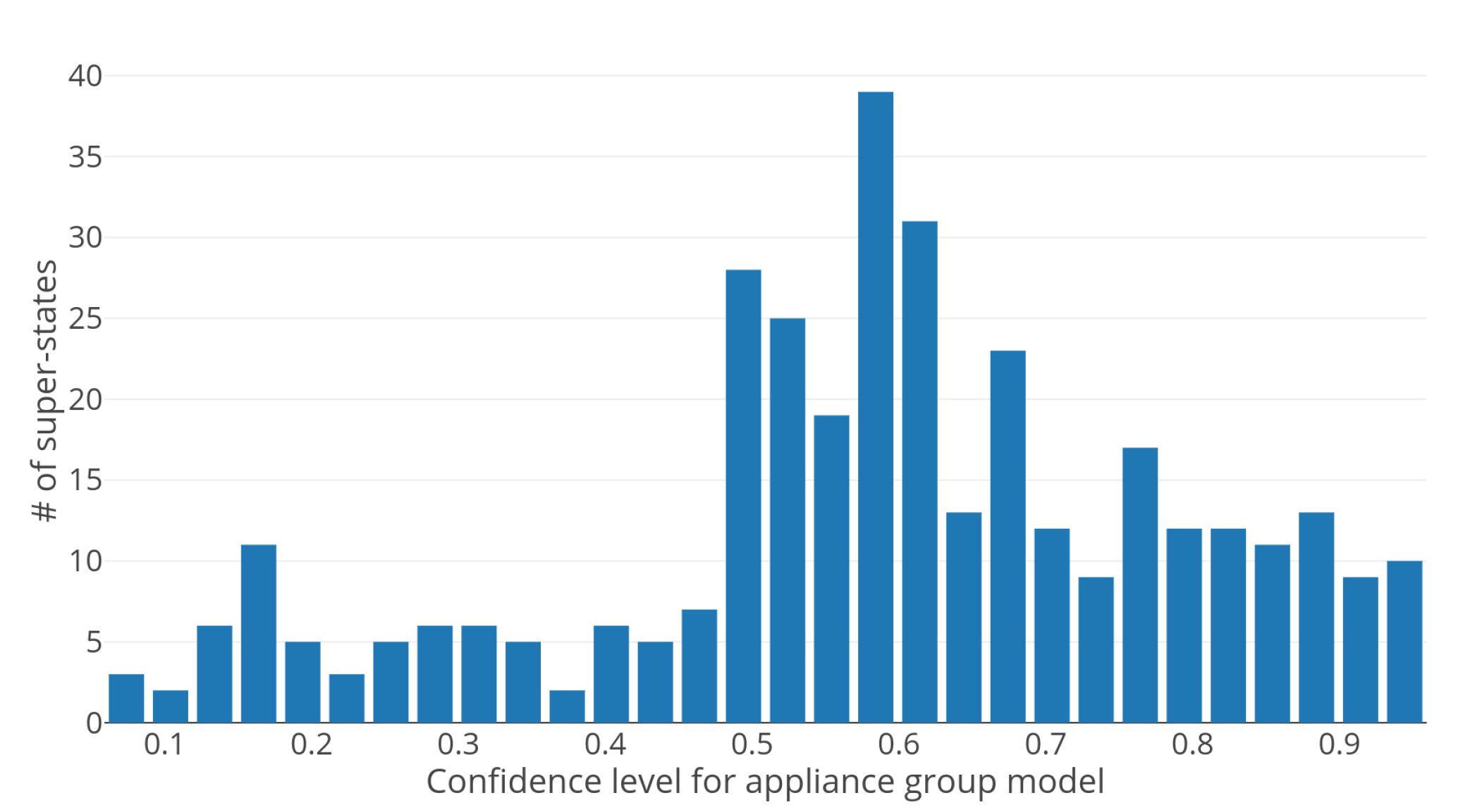
4.3.1. Appliance Group Model

The architecture of the appliance group model consists of seven hidden layers with ReLU [44] activation function, and the size of hidden layers are shown in

Table 1. Hyper-parameters of multi-layer perceptron networks.

Layer 1	Layer 2	Layer 3	Layer 4	Layer 5	Layer 6	Layer 7
20	40	60	80	71	118	256
5	10	×	×	×	×	×
10	40	200	256	×	×	×

, line 1. And the test result is shown in Figures 8–10.

4.3.2. User Model

The hyper-parameters for the temporal information embedding network in Section 3.1.1 and the decoding network in Section 3.1.3 are shown in Table 1, line 2 and line 3 respectively. A bigger $win\text{\_}size$ in Section 3.1.2 is important in preserving longer-term dependencies. In this work, we have tested the user model with different $win\text{\_}size$ as shown in Figure 4. As $win\text{\_}size$ increases, the performance of the model increases. However, when the $win\text{\_}size$ is bigger than 18, the performance is not improved hence the $win\text{\_}size$ is set to 18 to achieve a trade-off between performance and complexity.

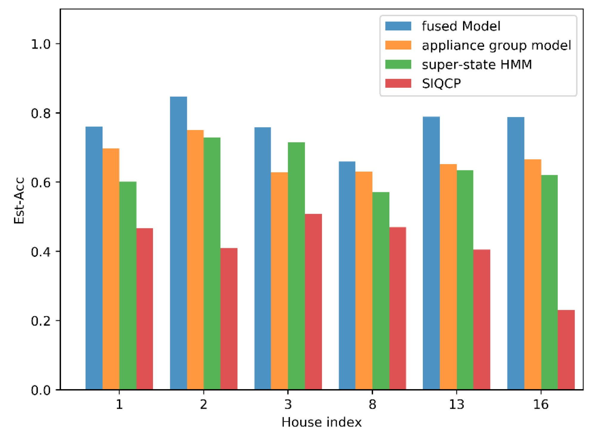
4.4. Performance of the Fused Model

4.4.1. Time Analysis

Figure 5 shows the calculation time of different methods. In conventional NILM methods, power consumption of appliances at only one time slice is updated each time, hence the computation time is proportional to the length of smart meter samples, and increases with the increase of sampling rate. However, appliances rarely change their states in short time scales. Hence in our method, we assume that the appliance states do not change in each $bin$. Each time one $bin$ is inferred, the power consumption of appliances in a period of time indicated by the $bin$ is updated (see Figure 6 and Figure 7). Considering that the average $delta\text{\_}time$ of each $bin$ is about 5 min, the method is more efficient than conventional methods in processing long power readings with high sampling rate.

4.4.2. Performance Evaluation

The performance of the proposed methodology is compared with two baseline models which are all state-of-the-art works in the literature of NILM, namely super-state HMM [3] and SIQCP [6]. The results are given in Figure 8, Figure 9 and Figure 10. It can be observed that the appliance group model outperforms SIQCP in terms of all metrics, however, the performance could be further improved when fused with the user model due to the introduction of user behavior sequential patterns and other user behavior pattern related information. However, compared with other houses, in house 2 and 3, the performance of the model is improved very little when combined with the user model, which indicates that the appliance usage behaviors in house 2, 3 may not following sequential patterns.

In the fused model, the probability of the given $bin$ belonging to each super-state is calculated by weighted sum of the two models, each model following a different assumption. And the importance of each model in detecting different super-states could be evaluated by the confidence level w in (16). In the REFIT dataset, we found that the detection of about 1/3 super-states is more dependent on the user model (see Figure 11), namely the usage habits, while the detection of others is more dependent on the appliance group model, namely the power consumption. We found that the recognition of high-power appliances relies more on the appliance group model, while the recognition of low-power appliances relies more on the user behavior model. The reason is that the low-power appliances has less impact on the aggregated power of all appliances, the appliance group model can hardly recognize the appliance according to the power consumption.

In most houses, the proposed model has outperformed all competing methods on all metrics. Considering more states of all appliances will make the appliance energy related metrics improved. For example, in the proposed method, the washing machine only has two states, that is, ON or OFF, corresponding to two power consumption, while the super-state HMM [3] considers that the washing machine has four states: off, wash, rinse, and spin, correspondings to four power consumption, which makes the ${\widehat{y}}_t^{\left(m\right)}$ in (4) near the actual appliance power consumption. However, the number of super-states in super-state HMM [3] is the product of the number of states of each appliance, making the model too big to be trained in a house with a large number of appliances. If the appliance works with steady power consumption, the power consumption estimation will be more accurate (such as appliances in house 3, 8), and vice versus. In addition, condensed representation will also have effect on the recognition of such appliances, which is further discussed in Section 4.6.

4.5. Testing with Different Proportions of Training Set

The deep learning is hungry for labeled data, but we may not get as much training data in practice. The larger the training set, the better the algorithm performs on the testing set, and vice versa. Figure 12 shows the performance of the algorithm when splitting the dataset with different percentages of training/testing data. House 1, 2, 3, 8, 13 and 16 contain labeled data for 406 days, 438 days, 454 days, 487 days, 556 days and 357 days, respectively. The f1-micros decrease rapidly when the training set proportion is less than about 20–40%, which indicates that we should collect at least 90 days of labeled data for training the deep learning based models in these houses.

4.6. Testing Continuous Varying Appliances

The condensed representation in Section 2.1 can improve the performance of recognizing appliances working with steady power consumption by preserving longer-term dependencies (see Figure 1). However, for continuous varying appliances, it is more difficult to choose the proper $\theta$ to balance the trade-off between assignment accuracy and long-term dependency, generally, the used event detection in Reference [9] will produce too many $bin$s even on a short sequence of power readings for continuous varying appliances, causing the model more difficult to be trained compared with steady power consumption appliances.

Table 2. Mean of F1 score of appliances.

	Freezer	Dryer	Washer	Computer	Heater	Cooking	TV	Others
Fused Model	0.88	0.98	0.93	0.90	0.99	0.97	0.82	0.96
Appliance Group Model	0.85	0.98	0.92	0.88	0.99	0.97	0.76	0.96
Super-state HMM	0.92	0.98	0.89	0.98	0.95	0.96	0.94	0.99
SIQCP	0.70	0.99	0.88	0.85	0.95	0.95	0.79	0.97

shows the averaged F1 score on each appliance in house 4, 5, 6, 7, 9, 10, 12, 14, 17, 18, 19 and 20. For continuous varying appliances such as freezer, computer and television, the F1 scores of the proposed method is relatively low, causing the super-state HMM [3] outperforms our method in these houses.

5. Conclusions and Future Work

This paper presented a novel NILM methodology by modeling the user and the appliances with DNNs separately. The user model is built to infer the current appliance usage behavior based on behaviors from the past several time intervals, which takes temporal information as well as long-term behaviors history to perform NILM. While the appliance group model could perform NILM with electrical characteristics and temporal information. These models are fused to achieve better NILM performance.

As mentioned in Section 1.3, there are three key factors that limit the deployment of NILM in practice. In this work, the computation efficiency is significantly improved by condensed representation and utilizing the parallel computing capability of GPUs. And 90 days of labeled data is required to achieve good generalization properties. The case study shows that the proposed NILM method has achieved good performance especially in terms of classification metrics especially on steady power consumption appliances.

Future works may focus on two aspects—(1) appliances usage forecasting. The user model in this work can predict the next appliance usage behavior based on behaviors from the past several time intervals, which could be used to perform short-term residential load forecasting; (2) improving the performance of NILM by integrating other data sources such as temperature or human sensors. (3) unsupervised/semi-supervised NILM algorithm. The NILM algorithm proposed in this paper requires a large amount of labeled data in the training phase, however, unsupervised/semi-supervised can train the NILM model with little or even no labeled data, which is of great significance to the application of NILM in practice.

References

1. Hosseini, S.S.; Agbossou, K.; Kelouwani, S.; Cardenas, A. Non-intrusive load monitoring through home energy management systems: A comprehensive review. Renew. Sustain. Energy Rev. 2017, 79, 1266–1274. [Google Scholar] [CrossRef]
2. Zhai, S.; Wang, Z.; Yan, X.; He, G. Appliance Flexibility Analysis Considering User Behavior in Home Energy Management System Using Smart Plugs. IEEE Trans. Ind. Electron. 2019, 66, 1391–1401. [Google Scholar] [CrossRef]
3. Makonin, S.; Popowich, F.; Bajić, I.V.; Gill, B.; Bartram, L. Exploiting hmm sparsity to perform online real-time nonintrusive load monitoring. IEEE Trans. Smart Grid 2016, 7, 2575–2585. [Google Scholar] [CrossRef]
4. Singhal, V.; Maggu, J.; Majumdar, A. Simultaneous Detection of Multiple Appliances from Smart-meter Measurements via Multi-Label Consistent Deep Dictionary Learning and Deep Transform Learning. IEEE Trans. Smart Grid 2018, 10, 2969–2978. [Google Scholar] [CrossRef] [Green Version]
5. Singh, S.; Majumdar, A. Deep Sparse Coding for Non-Intrusive Load Monitoring. IEEE Trans. Smart Grid 2018, 9, 4669–4678. [Google Scholar] [CrossRef] [Green Version]
6. Kong, W.; Dong, Z.Y.; Ma, J.; Hill, D.; Zhao, J.; Luo, F. An Extensible Approach for Non-Intrusive Load Disaggregation with Smart Meter Data. IEEE Trans. Smart Grid 2017, 9, 3362–3372. [Google Scholar] [CrossRef]
7. Welikala, S.; Dinesh, C.; Ekanayake, M.P.B.; Godaliyadda, R.I.; Ekanayake, J. Incorporating Appliance Usage Patterns for Non-Intrusive Load Monitoring and Load Forecasting. IEEE Trans. Smart Grid 2017, 10, 448–461. [Google Scholar] [CrossRef]
8. Liu, Y.; Geng, G.; Gao, S.; Xu, W. Non-Intrusive Energy Use Monitoring for a Group of Electrical Appliances. IEEE Trans. Smart Grid 2016, 9, 3801–3810. [Google Scholar] [CrossRef]
9. Iwayemi, A.; Zhou, C. SARAA: Semi-supervised learning for automated residential appliance annotation. IEEE Trans. Smart Grid 2017, 8, 779–786. [Google Scholar] [CrossRef]
10. Houidi, S.; Fourer, D.; Auger, F. On the Use of Concentrated Time–Frequency Representations as Input to a Deep Convolutional Neural Network: Application to Non Intrusive Load Monitoring. Entropy 2020, 22, 911. [Google Scholar] [CrossRef]
11. Jazizadeh, F.; Becerik-Gerber, B.; Berges, M.; Soibelman, L. An unsupervised hierarchical clustering based heuristic algorithm for facilitated training of electricity consumption disaggregation systems. Adv. Eng. Inform. 2014, 28, 311–326. [Google Scholar] [CrossRef]
12. Tabatabaei, S.M.; Dick, S.; Xu, W. Toward non-intrusive load monitoring via multi-label classification. IEEE Trans. Smart Grid 2017, 8, 26–40. [Google Scholar] [CrossRef]
13. Liang, J.; Ng, S.K.; Kendall, G.; Cheng, J.W. Load signature study Part 1 Basic concept, structure, and methodology. IEEE Trans. Power Deliv. 2010, 25, 551–560. [Google Scholar] [CrossRef]
14. Mengistu, M.A.; Girmay, A.A.; Camarda, C.; Acquaviva, A.; Patti, E. A Cloud-based On-line Disaggregation Algorithm for Home Appliance Loads. IEEE Trans. Smart Grid 2018, 10, 3430–3439. [Google Scholar] [CrossRef]
15. Cominola, A.; Giuliani, M.; Piga, D.; Castelletti, A.; Rizzoli, A.E. A hybrid signature-based iterative disaggregation algorithm for non-intrusive load monitoring. Appl. Energy 2017, 185, 331–344. [Google Scholar] [CrossRef]
16. Parson, O.; Ghosh, S.; Weal, M.J.; Rogers, A. Non-Intrusive Load Monitoring Using Prior Models of General Appliance Types. In Proceedings of the Twenty-Sixth Conference on Artificial Intelligence (AAAI-12), Toronto, ON, Canada, 22–26 July 2012. [Google Scholar]
17. Guo, Z.; Wang, Z.J.; Kashani, A. Home appliance load modeling from aggregated smart meter data. IEEE Trans. Power Syst. 2015, 30, 254–262. [Google Scholar] [CrossRef] [Green Version]
18. Aquino, A.L.L.; Ramos, H.S.; Frery, A.C.; Viana, L.P.; Cavalcante, T.S.G.; Rosso, O.A. Characterization of electric load with Information Theory quantifiers. Phys. A Stat. Mech. Its Appl. 2017, 465, 277–284. [Google Scholar] [CrossRef]
19. Kim, H.; Marwah, M.; Arlitt, M.; Lyon, G.; Han, J. Unsupervised disaggregation of low frequency power measurements. In Proceedings of the 2011 SIAM International Conference on Data Mining; SIAM: Philadelphia, PA, USA, 2011; pp. 747–758. [Google Scholar]
20. Jiang, L.; Luo, S.; Li, J. An Approach of Household Power Appliance Monitoring Based on Machine Learning. In Proceedings of the 2012 Fifth International Conference on Intelligent Computation Technology and Automation, Zhangjiajie, China, 12–14 January 2012; pp. 577–580. [Google Scholar] [CrossRef]
21. Kelly, J.; Knottenbelt, W. Neural nilm: Deep neural networks applied to energy disaggregation. In Proceedings of the 2nd ACM International Conference on Embedded Systems for Energy-Efficient Built Environments, Seoul, Korea, 4–5 November 2015; pp. 55–64. [Google Scholar]
22. Nguyen, M.; Alshareef, S.; Gilani, A.; Morsi, W.G. A novel feature extraction and classification algorithm based on power components using single-point monitoring for NILM. In Proceedings of the 2015 IEEE 28th Canadian Conference on Electrical and Computer Engineering (CCECE), Halifax, NS, Canada, 3–6 May 2015; pp. 37–40. [Google Scholar]
23. Kolter, J.Z.; Jaakkola, T. Approximate inference in additive factorial hmms with application to energy disaggregation. In Proceedings of the Fifteenth International Conference on Artificial Intelligence and Statistics, La Palma, Canary Islands, Spain, 21–23 April 2012; pp. 1472–1482. [Google Scholar]
24. Chen, Z.; Wu, L.; Fu, Y. Real-time price-based demand response management for residential appliances via stochastic optimization and robust optimization. IEEE Trans. Smart Grid 2012, 3, 1822–1831. [Google Scholar] [CrossRef]
25. Liu, H. Appliance Identification Based on Template Matching. In Non-intrusive Load Monitoring; Springer: Berlin/Heidelberg, Germany, 2020; pp. 79–103. [Google Scholar]
26. D’Incecco, M.; Squartini, S.; Zhong, M. Transfer learning for non-intrusive load monitoring. IEEE Trans. Smart Grid 2019, 11, 1419–1429. [Google Scholar] [CrossRef] [Green Version]
27. Bishop, C.M. Pattern Recognition and Machine Learning (Information Science and Statistics); Springer: Secaucus, NJ, USA, 2006. [Google Scholar]
28. Li, D.; Bissyandé, T.F.; Kubler, S.; Klein, J.; Le Traon, Y. Profiling household appliance electricity usage with n-gram language modeling. In Proceedings of the 2016 IEEE International Conference on Industrial Technology (ICIT), Taipei, Taiwan, 14–17 March 2016; pp. 604–609. [Google Scholar]
29. Murray, D.; Stankovic, L.; Stankovic, V. An electrical load measurements dataset of United Kingdom households from a two-year longitudinal study. Sci. Data 2017, 4, 160122. [Google Scholar] [CrossRef] [Green Version]
30. Pipattanasomporn, M.; Kuzlu, M.; Rahman, S.; Teklu, Y. Load profiles of selected major household appliances and their demand response opportunities. IEEE Trans. Smart Grid 2014, 5, 742–750. [Google Scholar] [CrossRef]
31. Zhou, C.; Bai, J.; Song, J.; Liu, X.; Zhao, Z.; Chen, X.; Gao, J. ATRank: An Attention-Based User Behavior Modeling Framework for Recommendation. arXiv 2017, arXiv:1711.06632. [Google Scholar]
32. Ioffe, S.; Szegedy, C. Batch normalization: Accelerating deep network training by reducing internal covariate shift. arXiv 2015, arXiv:1502.03167. [Google Scholar]
33. Goodfellow, I.; Bengio, Y.; Courville, A. Deep Learning; MIT Press: Cambridge, MA, USA, 2016; Available online: http://www.deeplearningbook.org (accessed on 28 October 2020).
34. Farnadi, G.; Tang, J.; De Cock, M.; Moens, M.F. User Profiling through Deep Multimodal Fusion. In Proceedings of the 11th ACM International Conference on Web Search and Data Mining, Marina Del Rey, CA, USA, 5–9 February 2018. [Google Scholar]
35. Zhang, Y.; Dai, H.; Xu, C.; Feng, J.; Wang, T.; Bian, J.; Wang, B.; Liu, T.Y. Sequential Click Prediction for Sponsored Search with Recurrent Neural Networks. AAAI 2014, 14, 1369–1375. [Google Scholar]
36. Hochreiter, S.; Schmidhuber, J. Long Short-Term Memory. Neural Comput. 1997, 9, 1735–1780. [Google Scholar] [CrossRef] [PubMed]
37. 2016. Available online: https://github.com/shi-yan/FreeWill/tree/master/Docs/Diagrams (accessed on 28 October 2020).
38. Sherstinsky, A. Fundamentals of Recurrent Neural Network (RNN) and Long Short-Term Memory (LSTM) Network. Phys. D Nonlinear Phenom. 2020, 404, 132306. [Google Scholar] [CrossRef] [Green Version]
39. Pascanu, R.; Mikolov, T.; Bengio, Y. On the difficulty of training recurrent neural networks. In Proceedings of the 30th International Conference on Machine Learning, ICML 2013, Atlanta, GA, USA, 16–21 June 2013; number PART 3. pp. 2347–2355. [Google Scholar]
40. Mikolov, T.; Sutskever, I.; Chen, K.; Corrado, G.S.; Dean, J. Distributed representations of words and phrases and their compositionality. In Advances in Neural Information Processing Systems; MIT Press: Cambridge, MA, USA, 2013; pp. 3111–3119. [Google Scholar]
41. Kingma, D.P.; Ba, J.L. Adam: Amethod for stochastic optimization. In Proceedings of the 3rd International Conference on Learning Representations (ICLR), San Diego, CA, USA, 7–9 May 2015. [Google Scholar]
42. Makonin, S.; Popowich, F. Nonintrusive load monitoring (NILM) performance evaluation. Energy Effic. 2015, 8, 809–814. [Google Scholar] [CrossRef]
43. Kolter, J.Z.; Johnson, M.J. REDD: A public data set for energy disaggregation research. In Proceedings of the Workshop on Data Mining Applications in Sustainability (SIGKDD), San Diego, CA, USA, 24 August 2011; Volume 25, pp. 59–62. [Google Scholar]
44. Nair, V.; Hinton, G.E. Rectified linear units improve restricted boltzmann machines. In Proceedings of the 27th International Conference on Machine Learning (ICML-10), Haifa, Israel, 21–24 June 2010; pp. 807–814. [Google Scholar]
Figure 1. Power consumption data from REFIT dataset [29]. The sampling rate is 1/3 Hz, hence, there are more than 100 samples in 400 s, which is too expensive in complexity to preserve long-term dependency. However, it could be much easier if the time series is represented by a short sequence with 8 b i n s.
Energies 13 05629 g001
Figure 2. Long Short-Term Memory (LSTM) block, the figure is referenced from Reference [37]. Each block is associated with one particular time instance by incorporating input x t into the block, and the block can be unfolded as a repetitive structure to integrate variable length sequences dynamically. Note that every block in the sequence share the same parameters.
Energies 13 05629 g002
Figure 3. Architecture of user model and how it is used to perform inference. The user model will encode the current bin (t, Δ t ), if an event is detected at t and last for Δ t time steps, and the recorded behaviors for duration of e m b e d d i n g _ s i z e time intervals to produce the probability of current observation belonging to each super-state assuming that appliances usage before the current time t is recorded.
Energies 13 05629 g003
Figure 4. Performance of the user model on REFIT dataset with different w i n _ s i z e s. Note that at each time, the t a r g e t s (see (6)) input to the model are the ground truth, not the estimated super-states. The user model can only get good performance when combined with the appliance group model, because the user model is sensitive to wrong NILM results at past time intervals, while the appliance group model can make the model less dependent on past NILM results.
Energies 13 05629 g004
Figure 5. Comparison of disaggregating time.
Energies 13 05629 g005
Figure 6. Appliance load profiles for house 1 in the REFIT dataset between 24 March 2014 06:00:00 and 24 March 2014 12:00:00.
Energies 13 05629 g006
Figure 7. Estimated appliance load profiles for house 1 in the REFIT dataset between 24 March 2014 06:00:00 and 24 March 2014 12:00:00.
Energies 13 05629 g007
Figure 8. Comparison of ACCs.
Energies 13 05629 g008
Figure 9. Comparison of f1-micros.
Energies 13 05629 g009
Figure 10. Comparison of E s t A c c .
Energies 13 05629 g010
Figure 11. The number of super-states within each appliance group model confidence interval. The confidence level near 1 indicates that the inference of the super-state depends more on the appliance group model, less on the user model, and vice versa.
Energies 13 05629 g011
Figure 12. Comparison of f1-micros with different training set proportions.
Energies 13 05629 g012