Abstract
The adoption of electric vehicles is incentivized by governments around the world to decarbonize the mobility sector. Simultaneously, the continuously increasing amount of renewable energy sources and electric devices such as heat pumps and electric vehicles leads to congested grids. To meet this challenge, several forms of flexibility markets are currently being researched. So far, no analysis has calculated the actual flexibility potential of electric vehicles with different operating strategies, electricity tariffs and charging power levels while taking into account realistic user behavior. Therefore, this paper presents a detailed case study of the flexibility potential of electric vehicles for fixed and dynamic prices, for three charging power levels in consideration of Californian and German user behavior. The model developed uses vehicle and mobility data that is publicly available from field trials in the USA and Germany, cost-optimizes the charging process of the vehicles, and then calculates the flexibility of each electric vehicle for every 15 min. The results show that positive flexibility is mostly available during either the evening or early morning hours. Negative flexibility follows the periodic vehicle availability at home if the user chooses to charge the vehicle as late as possible. Increased charging power levels lead to increased amounts of flexibility. Future research will focus on the integration of stochastic forecasts for vehicle availability and electricity tariffs.
1. Introduction
Scarcity of fossil fuels, oil price fluctuations, and increased awareness of the negative impacts caused by anthropogenic climate change have led to an increasing use of variable renewable energy (VRE) sources. With the agreed goal of limiting anthropogenic global warming to well below 2 degrees Celsius, this trend is expected to continue and even accelerate. While hydropower and biomass are, in their operational behavior comparable to conventional power plants, the power generation of photovoltaic and wind systems is variable, and generation prediction challenging and subject to uncertainty. Introducing flexibility products to the power system is one measure to cope with this variability and uncertainty.
Ma et al. define flexibility as the “the ability of a power system to cope with variability and uncertainty in both generation and demand, while maintaining a satisfactory level of reliability at a reasonable cost, over different time horizons” [1]. While this definition describes the general characteristic of flexibility, the Union of the Electricity Industry—Eurelectric—defines flexibility in a more application-oriented way, as “the modification of generation injection and/or consumption patterns in reaction to an external signal (price signal or activation) in order to provide a service within the energy system. The parameters used to characterize flexibility include the amount of power modulation, the duration, the rate of change, the response time, the location, etc.” [2].
Nowadays, large-scale flexibility products with a capacity greater than 1 MW are widely used to stabilize grid frequency. On the supply side, system operators (SO) use measures such as redispatch and feed-in management. On the demand side, they use sheddable loads and industrial demand-side-management as grid ancillary services [3,4,5]. While regulation and various market designs for energy trading already exist, academic and industrial research now focus on introducing unique flexibility platforms [6]. Such new platforms will allow residential consumers and prosumers to participate with their distributed energy resources (DER)—such as combined-heat-and-power units (CHP), electric vehicles (EV), residential heat pumps (HP), photovoltaic systems (PV), and battery storage units—as well as large industrial parties to offer flexibility [7,8,9]. In the future, SO will be able to manage grid congestions in a less resource-intensive manner and potentially avoid costly grid expansions and the curtailment of VRE [10,11]. Such flexibility platforms differ from existing energy market mechanisms in that they trade power instead of energy. SOs place their flexibility demand on the platform and are matched with residential and industrial flexibility providers.
Flexibility can be both negative and positive. Negative flexibility refers to the delay of grid feed-in or the consumption of non-scheduled energy. Positive flexibility is the delay of grid energy consumption or the non-scheduled grid feed-in.
Home energy management systems (HEMS) can quantify, price, and offer flexibility from private DER to such platforms and re-schedule devices based on the platform response. Beaudin et al. conclude that an HEMS is a demand response tool with the goal of optimizing consumption and production profiles in a house that communicates with household devices, utilities, and forecasting service provider [12]. The most important components of such a system required for calculating flexibility offers are visualized in Figure 1.
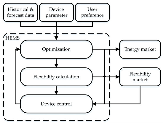
Figure 1.
Generalized structure of an HEMS. Historical and forecast data refers to weather data, historical consumption and production data and expected energy prices.
A review of HEMS concluded that cost optimization is the most frequently implemented objective function [12]. Yan et al. state that price-driven demand response is an important demand response measure [13]. Therefore, the type and structure of the electricity price signal is of crucial importance for the optimization problems of HEMSs.
Eurelectric differentiates fixed-priced offers and various types of dynamic pricing [14]. Nowadays, the majority of residents in the US, for example, have a fixed-priced electricity tariff [15]. Besides fixed-priced offers, utilities offer different types of dynamic pricing: time-of-use (ToU), real-time pricing (RTP), and others, such as critical peak pricing (CPP). ToU tariffs offer static pricing schemes with pre-defined prices for specified periods and seasons. As such, ToU tariffs are easy to follow for any customer, however, for the SO they run the risk of creating demand peaks of higher magnitude than the ones caused by fixed-priced offers [13]. In RTP, prices vary over short periods and are communicated to customers one day or less in advance. California was one of the first states to introduce RTP, in 1985 [16]. Nowadays, only a few RTP programs, such as ComEd’s Hourly Pricing, exist because they are technically difficult to implement and hard for customers to understand. A lot of studies have investigated the impact of different electricity tariffs on the peak demand of a distribution grid and concluded that simple ToU strategies can lead to increased peak demand [17,18]. However, the literature rarely discusses the impact of different electricity tariffs on flexibility.
Zade et al. published an HEMS model that optimizes the charging process of an electric vehicle (EV), and calculates the flexibility based on synthetic electricity prices, vehicle availabilities, and energy demands [9]. In order to analyze the realistic flexibility potential of EVs in a distribution grid, this paper describes a detailed case study conducted with vehicle field trial data from California, USA and Germany, three electricity tariffs, two controller strategies, and three charging power levels.
2. Materials and Methods
Figure 1 provides a functional overview of the generalized structure of an HEMS. As defined above, the primary objective of the HEMS is to fulfill the electricity, heat, and mobility demand of the household. For this purpose, the HEMS retrieves historical load profiles from an internal database and various other input data, e.g., user preferences, weather, and price forecasts from external sources. Then, an optimizer inside the HEMS calculates cost-optimal operating strategies for all controllable devices. Based on those operating schedules, the HEMS buys and sells energy on the energy market. Afterwards, the HEMS can offer deviations from the cost-optimal operating strategy as flexibility to SOs via a flexibility platform.
2.1. Input Data, Generation, and Consumption Forecast
The HEMS receives data from various parties, e.g., household inhabitants, forecast providers and weather stations. In an initial configuration step, household inhabitants insert device parameters like the charging station’s maximal charging power, or EV’s battery capacity, etc. More frequently, inhabitants update operational constraints, such as the daytime when an EV needs to be fully charged or the room temperature they find comfortable. Besides those user inputs, the HEMS is fed with different forecasts such as the upcoming weather conditions and expected energy prices. Finally, the optimization is triggered whenever new input data arrives or a certain amount of time has passed.
2.2. Optimization Approach
The calculation of the cost-optimal charging schedule is based on [19] but has been modified in order to incorporate constraints such as EV availabilities over time. This section describes the mixed-integer linear programming (MILP) model that has been used to calculate the cost-optimal charging schedule. In this work, it is assumed that the prosumer prefers a cost-optimized solution to the scheduling problem. Therefore, the target function in Equation (1) is formulated as a cost minimization.
Here is the set of time steps (t) considered throughout the scheduling horizon. is the duration of each time step, and are the electrical import and export power, while and are the corresponding electricity costs or revenues. and denote the volume of natural gas used and its specific cost, respectively. represents a penalty coefficient that is multiplied with the variable which is the difference between the desired final state of charge (SoC) and the actual SoC at the end of charging. This penalty term allows the optimizer to create a feasible problem even though the available time is not sufficient to charge a vehicle fully. Thereby, infeasible problems are avoided.
In addition, the energy balance and constraints for each appliance are critical to reflect a correct and realistic optimization. The constraints are as follows. The energy balance for electricity is represented by Equation (2) and for heat by Equation (3).
represent the electrical and thermal load of the household. is the power of one specific device, which belongs to one of the flexible appliance groups or . The group includes electric vehicles (EV), combined heat and power (CHP), heat pumps (HP), photovoltaic (PV), and battery systems (Bat). The group covers CHP, HP and thermal energy storages (TES). CHPs and HPs are classified into both groups because CHP produce electricity and heat at the same time and heat pump can convert power to heat.
For each flexible appliance and storage system, multiple constraints exist concerning their operation. Because this paper focuses on the quantification of flexibility of EVs, Equations (4)–(10) only list the constraints for EVs.
In Equations (4)–(7), represents the SoC of the EV battery. denotes the initial SoC of the EV, and are minimal and maximal SoC. refers to the SoC at time step zero and represents the SoC at the last available time step. may be reduced by if the time the vehicle is parked at home is not sufficient to charge the battery from start SoC to the desired end SoC. and refer to the start and end time of each availability period of the EV. is the battery capacity, is the charging power of the EV, and is the charging efficiency. is a variable that covers the power demand if the EV is available for multiple periods and energy has been discharged from the battery in between.
Equations (8)–(10) describe the constraints for . describes the vehicle availability for charging, which is 1 between and , and otherwise zero. Integrated into Equation (8), the availability does not allow the charging power to be greater than 0 if the vehicle is not available for charging. If the vehicle is available for charging, the charging power can be as high as the maximal charging power .
The formulated MILP model can be solved using commercial and open-source solvers, such as GLPK or Gurobi. Depending on the problem complexity, a conventional computer (e.g., Intel i7, 4 Cores, 24 GB RAM) presents a solution within a few seconds.
After optimizing the device’s operating strategy, a market agent in the HEMS trades its excess and required energy on the energy market and a controller schedules the device’s operation accordingly. After successful interaction with the energy market, the HEMS can start the flexibility calculation.
2.3. Flexibility Offers
Based on the optimal operating strategy of the devices described in the previous subsection, the HEMS calculates flexibility offers. Such a flexibility offer consists of the flexible power they can offer, the duration they can offer it, at what time, at which position in the grid, and at what price. The following subsections describe the calculation of these parameters in detail.
2.3.1. Location, Negative, and Positive Flexibility
Since in the setting considered here all flexible devices are stationary, the location of a flexible device is considered to be constant and is described by a unique identifier. In Germany, the Bundesnetzagentur introduced a 11-digit identifier (MaLo-ID: market location identifier) to simplify the market communication. Therefore, each HEMS that offers flexibility must attach the MaLo-ID to their bids.
Generally, all flexible devices are able to offer positive and negative flexibility, some even at the same time. For example, an EV charging station can offer positive flexibility by stopping an ongoing charging process or by reducing the charging power. Negative flexibility can be offered by charging a vehicle even though it has not been scheduled or by increasing the charging power while charging.
2.3.2. Power, Duration, and Energy
The DERs have different operating types. For both operating types, flexibility can be determined using Equations (11) and (12).
As mentioned in Section 2.2, denotes the power of the electricity consumer (C) and generator (G). is the maximal power of each flexible device. and represent the resulting positive and negative flexibility power for each device. Note that the positive and negative flexibility power is always positive and negative, respectively, or zero. As described above, one device can offer positive and negative flexibility at the same time.
Equations (13)–(15) describe the duration that flexibility is available. is the maximal duration that flexibility can be offered by a flexible device.
s.t.
This optimization problem is solved for each time step. The start time of each flexibility is exactly the time step chosen by each iteration. is variable in this problem and should be maximized without violating constraints and , which are abstracted from the equality and inequality constraints discussed in Section 2.2, respectively. Subscript for and indicates that the constraints shall be satisfied in the whole domain of is the positive or negative power of one specific flexible appliance, whereas refers to all other flexible appliances that still follow the cost-optimal schedules.
Once the flexibility duration has been acquired, the flexible energy is calculated by Equation (16).
Hence, the duration for which flexibility can be offered depends on the device’s current state. In the case of an EV, the flexibility that can be offered depends on the battery’s SoC, maximal charging power and availability.
In a final step, the flexibility would need a price tag in order to be offerable on a flexibility platform. However, this paper focuses on the quantification of flexibility of EVs and therefore the pricing is excluded from this analysis. Nevertheless, one possible pricing mechanism for flexibility of EV is described in [9].
Finally, the HEMS transfers the calculated flexibility parameters to a flexibility platform and waits for flexibility calls. Once a provider is called for flexibility, user preferences change, or new forecasts are available, the HEMS reinitiates the entire procedure from optimization to flexibility calculation and updates the offers on the flexibility platform.
The model is open-source and accessible via the link in the Supplementary Material.
3. Case Study
Figure 2 visualizes the general design of the case study. In a first step, we computed vehicle availabilities based on field trial data, collected by the California Department of Transportation and the Karlsruhe Institute of Technology. After gathering and pre-processing the vehicle availabilities and electricity tariffs, the cost-optimal charging schedules and the flexibility for each vehicle availability is calculated using the model described in Section 2. In order to analyze the aggregated flexibility potential of more than 4000 Californian and more than 11,000 German vehicle availabilities, the final results are aggregated. The following paragraphs describe the case study setup in detail. The link in the Supplementary Material contains an open-source script for the case study.
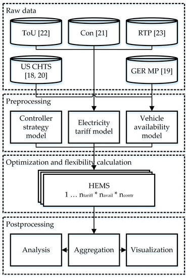
Figure 2.
Case study design, US CHTS, and GER MP refers to the Californian and German field trial data used to calculate the vehicle availabilities [18,19,20]. Con refers to the constant electricity rate in California [21], ToU refers to the ‘ToU-D-Prime’ electricity tariff of Southern California Edison [22], and RTP refers to the Hourly Real-Time prices of ComEd in Illinois [23], US.
refers to the number of electricity tariffs, refers to the number of vehicle availabilities, and refers to the number of controller strategies investigated in this case study.
3.1. Data Input and Preprocessing
For the case study, vehicle availabilities at home are computed based on the data sets of the Californian Household Travel Survey (US CHTS) and the German Mobility Panel (GER MP) [20,21]. Table 1 summarizes the parameters that characterize a vehicle availability.

Table 1.
Vehicle availability characterizing parameters.
The following subsections provide a brief summary of the most important characteristics and differences of the data sets used, as well as a short analysis of the computed vehicle availabilities.
3.1.1. Californian Household Travel Survey
Between February 2012 and March 2013, 677 Californian vehicles were equipped with in-vehicle GPS tracking devices. Every trip made by each vehicle was tracked for one week. The publicly available data set contains information about start and end times, start and end location, average speed and miles driven for every trip [22]. In the data set, 19,075 trips by 662 unique vehicles are recorded. The distance traveled varies from less than 0.5 km up to 1289 km. The average distance traveled is 35 km for all conducted trips (see Table 2). Start and end locations are categorized in four categories: HOME, WORK, SCHOOL, and OTHER.
Table 2.
Mean, maximum, minimum and 95%-ile of distance traveled since last departure from home.
Based on these parameters, the availability of vehicles at ‘HOME’ can be extracted, with arrival and departure time. Furthermore, the distance traveled is used to calculate the energy used by an average vehicle from its last departure from home. This procedure results in 4062 vehicle availabilities of 592 unique vehicles that contain a vehicle identifier, the distance traveled since the vehicle’s last departure from home, its arrival time at and departure time from home. Inconsistencies in the GPS data set, e.g., a vehicle arrives at home but departs for the next trip from another location, are neglected in this analysis.
3.1.2. German Mobility Panel
Between September and November 2017, 3867 persons from 1881 households logged their daily mobility behavior in a travel diary. After plausibility checks conducted by the Karlsruhe Institute of Technology (KIT), a total of 70,252 trips were gathered from 1850 persons [21]. The final trip data set includes information about the date, the trip’s start and end time, purpose, mode of transport used, duration, distance, and household. In 33,250 of the 70,252 trips logged, the person recorded having driven a vehicle as a driver either as a first, second or third “mode of transport used”. In 13,550 of the 33,250 trips, the purpose of the trip was to return home.
Based on the 33,250 trips, a total of 11,458 vehicle availabilities at home are computed by considering household and person identifier, trip purpose, and the trips’ chronology.
3.1.3. Vehicle Availabilities
In this subsection, the calculated vehicle availabilities are visualized and analyzed. In order to analyze the number of available vehicles at home during an average week, all vehicle availabilities are summed up for each time step of the week. Thereafter, the sums are averaged over all weeks of the field trials. Figure 3 shows the results for the Californian and German data sets. The average number of vehicles available in the Californian data set is 4.5 vehicles and for the German data set 21.3 vehicles. This can be explained by the compressed German field trial period of three months and the higher number of field trial participants (see [20,21]). Despite the differences in quantity, the vehicle availabilities indicate the same trends. At night, the number of vehicles increases until 12 a.m. and then decreases until 12 p.m. This behavior is repeated every day of the week. On weekends, however, the magnitude of the oscillation decreases approximately by a factor of three.
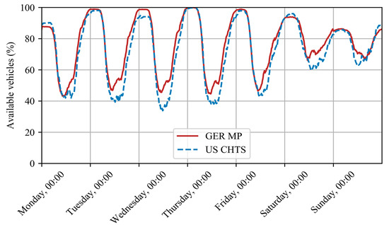
Figure 3.
Percentage of vehicles available at home during an average week. The maximum number of vehicles available at home is 6 for the US CHTS data and 120 for the GER MP.
Figure 4 visualizes a histogram of the total number of available vehicles over the distance traveled since their last departure from home. The results of both data sets show an exponential decay with only a few outliers. Ninety-five percent of the American and German vehicles arrive at home with less than 130 km driven since their last departure from home (see Table 2).
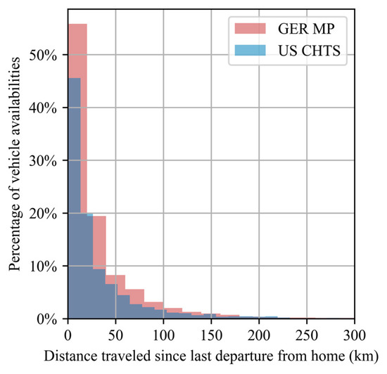
Figure 4.
Distribution of the distance traveled since the vehicle’s last departure from home—sampled from all modeled vehicle availabilities.
Figure 5 visualizes a relative frequency histogram of the total number of vehicles over the period the vehicles are available at home. Both data sets (US CHTS and GER MP) indicate a periodic behavior with a decreasing amplitude for an increasing time of availability. Most vehicles are available either for less than 1 to 3 h or for 7 to 25 h. Far fewer vehicles are available for 4 to 6 h or for more than 25 h. Table 3 summarizes the mean, maximum, minimum and 95%-ile of the available time for both data sets.
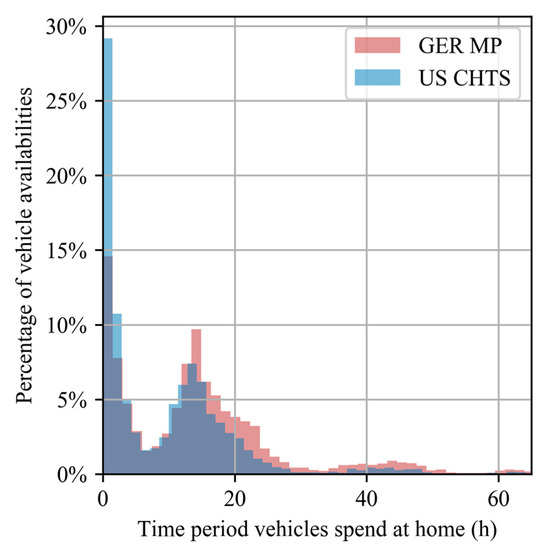
Figure 5.
Distribution of the time period vehicles spend at home—sampled from all modeled vehicle availabilities.
Table 3.
Mean, maximum, minimum, and 95%-ile of time of availability at home.
Figure 6 visualizes the distribution of the number of vehicles arriving at home over the hour of the day and the day of the week. Most vehicles arrive at home during the afternoon hours from 3 to 6 p.m. and depart from home between 6 and 9 a.m. Vehicles arrive at and depart from home more frequently during the week than on the weekend. Neither result is surprising considering conventional 9 to 5 working hours.
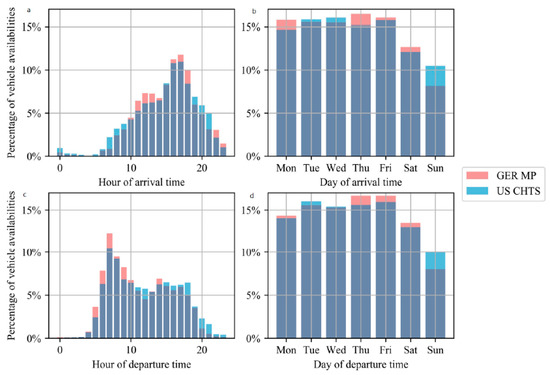
Figure 6.
Percentage of vehicle availabilities over (a) hour, (b) day of arrival time, (c) hour, and (d) day of departure time.
3.1.4. Electricity Tariffs
In order to quantify the impact of different electricity tariffs on the flexibility potential of electric vehicles, three tariffs are used in this case study.
The first tariff is a constant tariff ‘Con’ in which the electricity price does not vary. The price is set to 0.19 $/kWh, which was the average electricity price in California in 2018 [23].
‘ToU’ tariffs are offered throughout the United States and in other countries to motivate the reduction of electricity consumption in peak demand periods. Southern California Edison offers multiple ToU tariffs for residential customers on their website. For the simulations, the ‘ToU-D-Prime’ tariff as published on the website in the beginning of 2020 has been used. The tariff differentiates between winter and summer, weekday and weekend, and hour of day. In the winter, weekdays and weekends are priced equally. Between 4 and 9 p.m. the mid-peak tariff is active during the entire winter (0.36 $/kWh) and on weekends in the summer (0.27 $/kWh). During the summer, on weekdays from 4 to 9 p.m., the on-peak tariff for 0.39 $/kWh is active. From 9 to 4 p.m. the off or super-off-peak tariff at 0.14 and 0.13 $/kWh is active. This tariff motivates customer to reduce their electricity consumption in the late afternoon and early evening.
The third tariff integrated in this analysis is RTP. California already implemented two RTP programs in 1985 and 1987. However, both RTP programs had been canceled by 2003 [16]. Nowadays, California only offers Con and ToU tariffs. Therefore, a publicly available RTP tariff from ComEd, an energy supplier in Illinois, US is chosen [24]. In order to equalize the electricity prices for all tariffs, is added to the real-time prices. is the equal to the constant electricity price of 0.19 $/kWh minus the mean of all RTP. Since an analysis of the forecasting error of RTP is beyond the scope of this publication, the RTP tariff is assumed to be a perfect forecast of the electricity prices.
3.1.5. Controller Strategies
In order to quantify the impact of different controller strategies or user preferences on the flexibility potential of electric vehicles, we implemented two controller strategies.
The first controller strategy is to charge the vehicle at minimal costs but as soon as possible. Such behavior can be simulated by adding a minimal price increment onto the electricity prices (see Equation (18)).
denotes the actual electricity prices/revenues and the term that is added in accordance with the controller strategy. In the case of the first controller strategy, minimal price increments are added in the range of 0.00001 to 0.00002 $/kWh and therefore do not affect the actual price of electricity for the user. In the case of constant electricity prices, the optimizer would choose the first possible time steps in order to charge at minimal costs. For the rest of this publication, this operating strategy is denoted as “+MI”.
In order to conserve battery life, a second controller strategy is to charge the vehicle as late as possible and therefore to keep the SoC of the EV battery as low as possible as long as possible. This controller strategy can be implemented either by the addition of a minimal price decrement in Equation (18) or in the optimizer by default. In our case, this behavior was implemented by default in the solver. Therefore, this controller strategy is not separately labeled.
Table 4 lists the five simulated operating strategies that represent the combination of the three electricity tariffs and the two controller strategies.
Table 4.
Simulated operating strategies that represent the combination of electricity tariffs and controller strategies.
3.2. Flexibility Calculation
In order to use the vehicle availabilities described in Section 3.1 as EV input parameters for the model described in Section 2, the energy demand is calculated based on the distance traveled. The energy required is the product of the specific energy consumption of the EV and the distance traveled .
For this case study, a specific energy consumption of 0.2 kWh/km is used for all vehicle availabilities [25,26]. Furthermore, the user preference for the desired SoC of the vehicle at the time of departure was set to 100 %. The charging efficiency is set to 98 %.
In order to investigate the impact of the maximal charging power, the maximal charging power is varied in three steps: . This variation allows all current and possible future residential charging station configurations to be analyzed.
While the HEMS is capable of calculating the flexibility of HP, CHP, PV, and batteries, all other possible inputs, such as additional electrical or thermal loads or generation, are set to zero.
For every one of the five operating strategies listed in Table 4 and every , the model calculates the optimal charging schedule and flexibility potential as a time series. This procedure resulted in a total of 165,870 for GER MP and 60,930 for US CHTS executions of the model.
3.3. Data Aggregation
Once optimal charging schedules and flexibility have been calculated for more than 15,000 vehicle availabilities for 5 operating strategies and 3 maximal charging powers, the results are aggregated.
First, all available vehicles, charging schedules, flexible power and energies are summed up for every time step of the field trial periods. The result is a data set that shows the total number of available vehicles at home, charging powers, flexible power and energy for every time step of the field trial.
In a final step, the summed data is clustered into weekly time steps (e.g., “Monday, 09:00”), and weekdays and weekends. The clusters are then averaged over the field trial duration.
4. Results
This chapter visualizes and describes the results of the case study in detail. The cost-optimal charging schedules are shown in the top two rows of plots, whereas the flexibility potential is shown in the bottom two rows of plots (Figure 7). The first section describes the cost-optimal charging schedules, and the second section the flexibility potentials of the vehicle availabilities from both data sets for the five operating strategies.
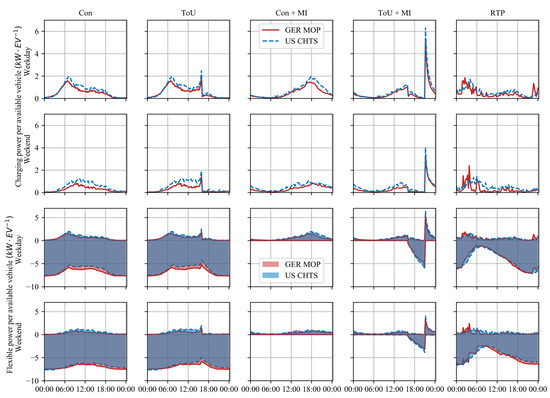
Figure 7.
The plot series visualizes the charging and flexible power per available EV. The first two rows of plots show the charging power per available EV for the five operating strategies on weekdays and weekends. The third and fourth rows of plots show the flexible power per available EV for the five operating strategies on weekdays and weekends.
4.1. Cost-Optimal Charging Schedules
In the top two rows of plots, Figure 7 shows the cost-optimal power demand per vehicle for weekdays in the first row and for weekends in the second row. The curves of the Con and the ToU operating strategy are almost identical and can only be distinguished by their behavior between 3 p.m. and 9 p.m. At 4 p.m., the ToU curves show a smaller second peak compared to the early morning hours. This behavior can be explained by the optimizer logic and mid/on-peak tariffs. The optimizer implemented charges the vehicles as late as possible and as cheaply as possible. Considering the mid/on-peak tariffs starting at 4 p.m., the optimizer schedules all vehicles that depart between 4 and 9 PM to charge right before 4 p.m. Therefore, this trend is consistent with the implemented optimizer logic. Besides the difference mentioned in the early afternoon, the power curves for the ToU and Con operating strategy show the same trend as visualized by the histogram of the departure times in Figure 6. The amplitude ranges from 0 to 2.5 kW/EV for both data sets. On weekends, the power ranges from 0 to 1.9 kW/EV and is more spread out throughout the day. Generally, the results indicate that the Californian vehicles require greater power per vehicle compared to the German vehicles.
The RTP operating strategy causes charging peaks that are spread out from 11 p.m. to 8 a.m. The peaks are more irregular than the ones for the Con and ToU operating strategies. While the power curves for the Con and ToU operating strategy indicate similar trends for the US CHTS and the GER MP data set, the cost-optimal charging power differ significantly between the German and the Californian data set in the RTP operating strategy. The charging power for the Californian data set looks rather smooth, whereas the results of the German vehicles look much spikier. Since the German data set was collected over a period of three months, a single drop in the real-time prices and the corresponding peak of charging power have a greater impact on the average charging power than those that occurred during the 12-month Californian field trial with only a few vehicles. However, the amplitude ranges also from 0 to 2.5 kW/EV for both data sets. Since real-time prices are much more difficult to forecast and exhibit erratic short-term changes, the demand peaks are most probably overestimated in these results.
The cost-optimal charging power for the operating strategy Con + MI indicates a shifted charging behavior. Whereas the Con operating strategy schedules vehicle charging right before their departure in the morning hours, the minimal price increments force the optimizer to charge the vehicles right after they arrive home. Therefore, the charging power curve for the Con + MI follows the almost Gaussian distribution of the arrival times shown in Figure 6. The amplitude ranges from 0 to 2 kW/EV, which is comparable to the curves of the Con and ToU operating strategies.
Nevertheless, ToU + MI cause the greatest charging power peaks (see Figure 7). Every day at 9 p.m., the optimizer schedules the vehicles that arrived between 4 and 9 p.m. to start charging at the same time. This leads to power peaks of more than 6 kW/EV for both data sets.
Overall, the US CHTS and the GER MP results show similar trends for the cost-optimal charging power for the five operating strategies simulated.
4.2. Flexibility
4.2.1. Operating Strategies
In the bottom two plots of Figure 7 the ranges of flexibility for the five operating strategies simulated are visualized.
For EVs, positive flexibility is equivalent to a pause or postponement of the charging process. Therefore, the upper boundary of the flexibility is equal to the optimal charging power.
According to the definition in Section 1, negative flexibility is the ability to consume electricity ahead of its schedule. Considering the operating strategy Con + MI and a cost optimization, no negative flexibility can be offered. Therefore, the lower boundary of the simulation results is congruent with the zero line (see Figure 7).
Similar to the aforementioned operating strategy, ToU + MI result in no negative flexibility between 9 p.m. and 4 p.m. From 4 p.m. to 9 p.m., the negative flexibility increases linearly as vehicles arrive home, and their charging process is scheduled from 9 p.m. onwards owing to lower electricity prices. At 9 p.m., negative flexibility drops back to zero.
The operating strategy Con and ToU result in almost identical negative flexibility results. Furthermore, the negative flexibility that can be offered follows the vehicle availability curves discussed in Section 3.1.3). Periodically, at night time, negative flexibility increases and reaches its maximum around 1 to 3 a.m. During the morning hours before 12 a.m., the flexibility decreases. Negative flexibility ranges from −5 kW/EV to −7.5 kW/EV with the Con and ToU operating strategies. On weekends, the ranges are smaller since vehicle fluctuations also decrease. At 4 p.m., the ToU operating strategy causes a minor drop in negative flexibility due to the charging of vehicles that depart between 4 and 9 p.m.
The RTP operating strategy also follows the vehicle availability described in Section 3.1.3). However, in contrast to the results of the ToU and Con operating strategies, the maximum negative flexibility is available right before midnight. After midnight, when electricity prices are the lowest, the vehicles are charged and the available negative flexibility decreases. On weekends, the range of negative flexibility that can be offered decreases slightly as the fluctuations in vehicle availabilities also decrease. The negative flexibility that can be offered ranges between −2 kW/EV and −7 kW/EV for both data sets. Therefore, RTP prices lead to less offerable negative flexibility than a Con or ToU operating strategy.
Having described the impact of the five operating strategies, the next subsections describe the impact of the maximal charging power on the offerable flexibility of EVs.
4.2.2. Maximal Charging Power
To analyze the impact of the maximum charging power level, the optimization and flexibility calculation for all vehicle availabilities are repeated for three maximum charging power levels: 3.7 kW, 11 kW, and 22 kW. Figure 8 shows the positive and negative flexible power that can be offered for the GER MP data set. Each operating strategy corresponds to a row and each maximum charging power level to a column of heat maps. Table 5 and Table 6 summarize the maximal flexible power and average flexible power for all five operating strategies. Generally, the positive flexibility is also representative of the cost-optimal charging power.
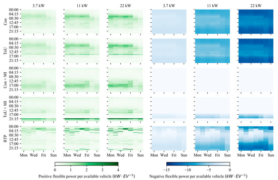
Figure 8.
Resulting positive and negative flexible power per available EV. These results are based on the GER MP vehicle availabilities, the five operating strategies {Con, ToU, Con + MI, ToU + MI, RTP}, and three maximal charging power levels {3.7, 11, 22 kW}.
Table 5.
Maximum and average positive flexible power for five operating strategies and three maximum charging powers.
Table 6.
Maximum and average negative flexible power for five operating strategies and three maximum charging powers.
The results of the ToU and Con operating strategy show similar behavior. As described in Section 4.1, the optimizer schedules EV chargings at the latest possible time. This leads to higher charging powers and a high level of positive flexibility from 3 a.m. to 8 a.m. on weekdays. A higher maximum charging power increases the maximal and average positive flexible power that can be offered (see Figure 8). However, the duration of positive flexibility seems to decrease with increasing maximum charging power in Figure 8. With a higher charging power level, the energy required is charged over a shorter time period, and therefore leads to a compressed availability of positive flexibility. The increase of maximal and average positive flexible power with an increasing maximum charging power can be explained by assuming that with a low charging power, e.g., 3.7 kW, not all vehicles are completely charged. In this case, the vehicle cannot offer any flexibility. With a higher maximum charging power, the charging station charges the EV over a shorter period and can therefore offer more flexibility. However, this relation is not linear, since the average positive flexible power seems to only change insignificantly from 11 to 22 kW. Therefore, the two observations described complement each other.
Considering the cost optimization described in IV.A, the results for positive flexible power for the ToU + MI, Con + MI, and RTP operating strategies indicate a similar behavior. With an increasing charging power, the positive flexible power that can be offered is compressed in time whereas the maximal power increases. Furthermore, the average quantity of positive flexibility increases (see Table 5). Both effects are explained in the previous paragraph.
Nevertheless, the ToU + MI and RTP operating strategies cause such high charging peaks at 9 p.m. (ToU + MI) and overnight (RTP) that the average maximal positive flexible power is three and two times higher than in the remaining operating strategies. Whereas the impact of the RTP might be overestimated since in a real-world scenario prices cannot be predicted as easily, the ToU + MI operating strategy can pose a major threat to grid stability.
Considering ToU and Con operating strategies, most negative flexibility can be offered at night and on weekends, when most vehicles are at home. Operating strategies with minimal price increments result in no flexibility (Con + MI) or only for short durations from 4 to 9 p.m. (ToU + MI). The causes have been discussed in the previous section. An RTP operating strategy shows similar trends as the ToU and Con operating strategies for weekdays. Most negative flexibility is offered at nighttime, from 5 p.m. to 3 p.m. On weekends, negative flexibility is at a high level and homogenously distributed for the Con and ToU operating strategy, whereas RTP results indicate a similar behavior as during the week. Such behavior can be explained by the time-varying electricity prices that are lower at nighttime throughout the entire week.
As discussed in the previous subsection the ToU, Con, and RTP operating strategies show similar trends in offerable negative flexibility. Table 6 displays the absolute differences between the operating strategies and the maximal charging power.
A variation in charging power results in an increase in maximal and average negative flexibility for all five simulated pricing scenarios. In order to identify a mathematical relationship between the maximum charging power and the amount of negative flexibility further simulations are required.
With all results summarize, the next chapter discusses the validity and limitations of the applied method.
5. Discussion
This paper presents a thorough analysis of cost-optimal charging schedules and flexibility potential of more than 15,000 vehicle availabilities at home for five operating strategies, and three maximal charging power levels. While the calculation of cost-optimal charging schedules is state of the art, the quantification and analysis of the available flexibility of EV complements and enhances existing literature.
In this analysis, perfect price forecasts have been used to analyze the flexibility of EVs. For the first four operating strategies, which were based on Con and ToU tariffs, the consideration of perfect price forecasts would not have led to any other results. However, in the case of RTP the effect of the perfect price forecast is not negligible. Since RTP cannot be forecasted precisely and multiple methods lead to a range of results, the absolute impact of RTP is expected to be smaller in reality. Therefore, future research will investigate the impact of the uncertainty of price forecasts on the flexibility that can be offered.
Overall, the ToU + MI operating strategy leads to the least favorable charging behavior and flexibility offers. The average charging power indicates major peaks at 9 p.m. and a smaller peak at 3:45 p.m. Both peaks are caused by the mid- and on-peak prices between 4 and 9 p.m. These peaks occur every weekday with similar power levels and therefore represent a significant stress for grid operation. The original assumption that the network could be relieved by time-varying discrete tariffs will become obsolete in the near future, when charging processes will be optimized and automated. This conclusion is in line with the existing literature [13,17]. Nevertheless, ToU operating strategies lead to the overall minimum charging costs compared to the other operating strategies (see Figure 9). Despite the seemingly cheaper ToU tariffs, regulators should omit operating strategies that offer pre-known price differences in the future for the sake of grid stability and security of supply.
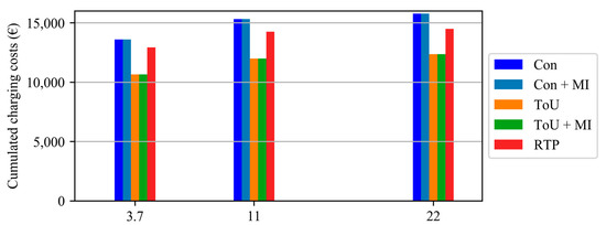
Figure 9.
Cumulated charging costs in € for five operating strategies and three maximum charging power levels. For this analysis, the 11,103 vehicle availabilities of the GER MP field trial were used.
In order to achieve grid-friendly user behavior and not to create further grid congestions, we will investigate the integration of local energy markets (LEM). LEM enable participants to trade and exchange their electricity locally. Market agents within HEMS predict the vehicle availability, post bids on the LEM, and adjust their bids automatically based on market results. With this approach, different prices are calculated locally, and users are motivated to consume electricity in times of high generation and to generate electricity in times of high demand.
For this case study, the most recent publicly available data sets with all required parameters were chosen. Since the field trial data was collected from a wide variety of households with different types of vehicles and only contain information about the distances traveled, departure and arrival times, the results can only be representative for realistic user behavior but not for specific types of vehicles. The energy demands of the vehicles were calculated based on the distances traveled. Even though the two data sets are not from the same year (2012/2013 and 2017), the results do not indicate any major differences. Furthermore, the report on the GER MP state that the trends in transportation and individual mobility have remained almost constant over the last 10 years [21]. Therefore, the effect of the different survey periods is considered insignificant. Nevertheless, the continuation of the coronavirus pandemic may mean that employees will be able to work from home to a greater extent, and that vehicle availability may therefore change in the long term. This effect has not yet been taken into account in this study but would be an interesting new aspect.
The gathered flexibility results of this case study are based on availabilities of vehicles at home. However, the method described is neither limited to those two regions nor to quantify flexibility based on EVs at home. This method is applicable to any region/data set that contains information about trip start and end times, purpose or start and end location of the trip, means of transport and distance travelled. Further investigations will investigate differences from other world regions and the quantification of flexibility at other locations, such as workplaces.
6. Conclusions
This paper describes in detail a model that calculates cost-optimal charging schedules and quantifies the flexibility of EV. A case study with more than 15,000 vehicle availabilities from Germany and the USA was conducted and the results visualized for weekdays, weekends, and an average week. Furthermore, the impact of five operating strategies and three charging power levels on the offerable flexibility were analyzed.
Based on these results, the following key findings can be drawn:
- ToU tariffs in combination with the user preference to charge the vehicle as soon as possible (ToU + MI) leads to significant increased grid congestions.
- Positive flexibility is mostly available during either the evening hours or early morning hours depending on the user’s preferred charging time (MI).
- No negative flexibility is available if the user is charged a constant electricity rate and chooses to charge as soon as possible (Con + MI).
- Negative flexibility follows the periodic availability of vehicle availabilities at home if the user chooses to charge the vehicle as late as possible (Con).
- Increased charging power levels lead to higher absolute positive and negative flexibility power levels and also increase the total offerable flexibility of EVs.
In conclusion, the model presented in Section 2 is able to quantify EV flexibility. Regulators, researchers, and system operators can use this model to investigate various influences such as tariff structures, user preferences, charging power levels etc. on the flexibility of EVs. Furthermore, the presented HEMS model can calculate the flexibility of heat pumps, combined heat and power, photovoltaic and battery systems. Once completed, this model will be a new helpful tool for tasks such as flexibility calculation, grid expansion planning, and the design and implementation of future electricity regulations.
Supplementary Materials
The model and the script to perform the ev case study is open-source and accessible via the following link: https://zenodo.org/badge/latestdoi/212816117.
Author Contributions
Conceptualization, M.Z.; data curation, M.Z.; formal analysis, M.Z. and P.T. funding acquisition, P.T. and U.W.; investigation, M.Z. and Z.Y.; methodology, M.Z. and Z.Y.; project administration, P.T. and U.W.; software, M.Z., Z.Y., and B.K.N.; supervision, P.T. and U.W.; validation, M.Z.; visualization, M.Z.; writing—original draft, M.Z. and Z.Y.; writing—review and editing, M.Z., Z.Y., B.K.N., P.T. and U.W. All authors have read and agreed to the published version of the manuscript.
Funding
The German Federal Ministry for Economic Affairs and Energy, Bundesministerium für Wirtschaft und Energie, funded this research under the grant number 03SIN109.
Conflicts of Interest
The authors declare no conflict of interest. The funders had no role in the design of the study; in the collection, analyses, or interpretation of data; in the writing of the manuscript, or in the decision to publish the results.
References
- Ma, J.; Silva, V.; Belhomme, R.; Kirschen, D.S.; Ochoa, L.F. Evaluating and Planning Flexibility in Sustainable Power Systems. IEEE Trans. Sustain. Energy 2012, 4, 200–209. [Google Scholar] [CrossRef]
- Eurelectric (2014)—Flexibility-and-Aggregation. 2014. Available online: https://www.usef.energy/app/uploads/2016/12/EURELECTRIC-Flexibility-and-Aggregation-jan-2014.pdf (accessed on 26 October 2020).
- Paulus, M.; Borggrefe, F. The potential of demand-side management in energy-intensive industries for electricity markets in Germany. Appl. Energy 2011, 88, 432–441. [Google Scholar] [CrossRef]
- Strbac, G. Demand side management: Benefits and challenges. Energy Policy 2008, 36, 4419–4426. [Google Scholar] [CrossRef]
- Zhou, K.; Yang, S. Demand side management in China: The context of China’s power industry reform. Renew. Sustain. Energy Rev. 2015, 47, 954–965. [Google Scholar] [CrossRef]
- Radecke, J.; Hefele, J.; Hirth, L. Markets for Local Flexibility in Distribution Networks. Kiel, Hamburg, 2019. Available online: https://www.econstor.eu/bitstream/10419/204559/1/Radecke%2C%20Hefele%20%26%20Hirth%202019%20%20Markets%20for%20Local%20Flexibility%20in%20Distribution%20Networks.pdf (accessed on 1 June 2020).
- Nalini, B.K.; Eldakadosi, M.; You, Z.; Zade, M.; Tzscheutschler, P.; Wagner, U. Towards Prosumer Flexibility Markets: A Photovoltaic and Battery Storage Model. In Proceedings of the 2019 IEEE PES Innovative Smart Grid Technologies Europe (ISGT-Europe), Bucharest, Romania, 29 September 2019–2 October 2019; pp. 1–5. [Google Scholar]
- You, Z.; Nalini, B.K.; Zade, M.; Tzscheutschler, P.; Wagner, U. Flexibility quantification and pricing of household heat pump and combined heat and power unit. In Proceedings of the 2019 IEEE PES Innovative Smart Grid Technologies Europe (ISGT-Europe), Bucharest, Romania, 29 September 2019–2 October 2019; pp. 1–5. [Google Scholar]
- Zade, M.; Incedag, Y.; El-Baz, W.; Tzscheutschler, P.; Wagner, U. Prosumer Integration in Flexibility Markets: A Bid Development and Pricing Model. In Proceedings of the 2018 2nd IEEE Conference on Energy Internet and Energy System Integration (EI2), Beijing, China, 20–22 October 2018; pp. 1–9. [Google Scholar]
- Kumar, A.; Srivastava, S.; Singh, S. Congestion management in competitive power market: A bibliographical survey. Electr. Power Syst. Res. 2005, 76, 153–164. [Google Scholar] [CrossRef]
- Yusoff, N.I.; Zin, A.A.M.; Bin Khairuddin, A. Congestion management in power system: A review. In Proceedings of the 2017 3rd International Conference on Power Generation Systems and Renewable Energy Technologies (PGSRET), Johor Bahru, Malaysia, 4–6 April 2017; pp. 22–27. [Google Scholar]
- Beaudin, M.; Zareipour, H. Home energy management systems: A review of modelling and complexity. Renew. Sustain. Energy Rev. 2015, 45, 318–335. [Google Scholar] [CrossRef]
- Yan, X.; Ozturk, Y.; Hu, Z.; Song, Y. A review on price-driven residential demand response. Renew. Sustain. Energy Rev. 2018, 96, 411–419. [Google Scholar] [CrossRef]
- Eurelectric—Union of the Electricity Industry. Dynamic Pricing in Electricity Supply. February 2017. Available online: http://www.eemg-mediators.eu/downloads/dynamic_pricing_in_electricity_supply-2017-2520-0003-01-e.pdf (accessed on 18 June 2020).
- Limmer, S. Dynamic Pricing for Electric Vehicle Charging—A Literature Review. Energies 2019, 12, 3574. [Google Scholar] [CrossRef]
- Barbose, G.; Goldman, C.; Neenan, B. A Survey of Utility Experience with Real Time Pricing; LBNL: Berkeley, CA, USA, 2004. [Google Scholar]
- Muratori, M.; Rizzoni, G. Residential Demand Response: Dynamic Energy Management and Time-Varying Electricity Pricing. IEEE Trans. Power Syst. 2015, 31, 1108–1117. [Google Scholar] [CrossRef]
- Veldman, E.; Verzijlbergh, R.A. Distribution Grid Impacts of Smart Electric Vehicle Charging From Different Perspectives. IEEE Trans. Smart Grid 2014, 6, 333–342. [Google Scholar] [CrossRef]
- Atabay, D. An open-source model for optimal design and operation of industrial energy systems. Energy 2017, 121, 803–821. [Google Scholar] [CrossRef]
- NuStats, L.L.C. 2010–2012 California Household Travel Survey: Final Report. June 2013. Available online: https://www.nrel.gov/transportation/secure-transportation-data/assets/pdfs/calif_household_travel_survey.pdf (accessed on 23 July 2020).
- Ecke, L.; Chlond, B.; Magdolen, M.; Hilgert, T.; Vortisch, P. Deutsches Mobilitätspanel (MOP): Wissenschaftliche Begleitung und Auswertung Bericht 2018/2019: Alltagsmobilität und Fahrleistung. Ger. Mobil. Panel 2020. [Google Scholar]
- California Department of Transportation. 2010–2012 California Household Travel Survey. National Renewable Energy Laboratory. Available online: https://www.nrel.gov/transportation/secure-transportation-data/tsdc-california-travel-survey.html (accessed on 23 July 2020).
- U.S. Energy Information Administration. 2018 Average Monthly Bill—Residential: (Data from forms EIA-861- schedules 4A-D, EIA-861S and EIA-861U). 2018. Available online: https://www.eia.gov/electricity/sales_revenue_price/pdf/table5_a.pdf (accessed on 23 July 2020).
- Commonwealth Edison Company. Comed’s Hourly Pricing Program. Available online: https://hourlypricing.comed.com/ (accessed on 23 July 2020).
- Electric Vehicle Database: Energy Consumption of Full Electric Vehicles. Available online: https://ev-database.org/cheatsheet/energy-consumption-electric-car (accessed on 23 July 2020).
- Hao, X.; Wang, H.; Lin, Z.; Ouyang, M. Seasonal effects on electric vehicle energy consumption and driving range: A case study on personal, taxi, and ridesharing vehicles. J. Clean. Prod. 2020, 249, 119403. [Google Scholar] [CrossRef]


Publisher’s Note: MDPI stays neutral with regard to jurisdictional claims in published maps and institutional affiliations. |
© 2020 by the authors. Licensee MDPI, Basel, Switzerland. This article is an open access article distributed under the terms and conditions of the Creative Commons Attribution (CC BY) license (http://creativecommons.org/licenses/by/4.0/).