Reliability Predictors for Solar Irradiance Satellite-Based Forecast

Abstract

The worldwide growing development of PV capacity requires an accurate forecast for a safer and cheaper PV grid penetration. Solar energy variability mainly depends on cloud cover evolution. Thus, relationships between weather variables and forecast uncertainties may be quantified to optimize forecast use. An intraday solar energy forecast algorithm using satellite images is fully described and validated over three years in the Paris (France) area. For all tested horizons (up to 6 h), the method shows a positive forecast skill score compared to persistence (up to 15%) and numerical weather predictions (between 20% and 40%). Different variables, such as the clear-sky index (K_c), solar zenith angle (SZA), surrounding cloud pattern observed by satellites and northern Atlantic weather regimes have been tested as predictors for this forecast method. Results highlighted an increasing absolute error with a decreasing SZA and K_c. Root mean square error (RMSE) is significantly affected by the mean and the standard deviation of the observed K_c in a 10 km surrounding area. The highest (respectively, lowest) errors occur at the Atlantic Ridge (respectively, Scandinavian Blocking) regime. The differences of relative RMSE between these two regimes are from 8% to 10% in summer and from 18% to 30% depending on the time horizon. These results can help solar energy users to anticipate—at the forecast start time and up to several days in advance—the uncertainties of the intraday forecast. The results can be used as inputs for other solar energy forecast methods.

1. Introduction

Since the year 2000, the cost of PV modules generation has significantly decreased, increasing the competitiveness of PV power against electricity generated from fossil fuels [1]. Concomitantly, financial incentives for the use of low-carbon energy have been established all over the world by various institutions. Consequently, the total PV capacity installed in the world has been multiplied by 14.4, from 40.2 GW in 2010 to 580.2 GW in 2019. During the same period, the total capacity of all renewable energies doubled from 1226.6 to 2536 GW [2]. The dramatic increase in PV production raises the issue of its massive penetration into the grid. The injection of any power source in the grid must be balanced at each instant by an equal consumption to ensure the safe and stable operation of the grid at a constant frequency.

However, the production of solar energy is essentially driven by the solar irradiance reaching the Earth’s surface, quantified as global horizontal irradiance (GHI). This physical quantity is highly variable for two main causes. The first one is astronomic: the irradiance depends deterministically on the diurnal and seasonal variations of solar elevation above the horizon. The second one is meteorological: atmospheric components (water vapor, aerosols and mainly clouds) significantly attenuate the solar radiation passing through the atmosphere and reaching a solar energy production system. In particular, cloud cover evolution above a given point is a stochastic process, thus, the derived GHI has a limited predictability [3].

Oversizing the PV capacity is one way to reduce this variability and the associated grid unbalancing risks. However, it wastes, through curtailment, a significant amount of produced energy and results in a limited penetration rate. Electricity storage is an obvious solution to limit this waste and increase the control of PV electricity injection into the grid. If current storage technologies are successfully used to control hybrid power supply—including PV—at micro-grid scales [4], it remains costly to develop sufficient capacity enabling a PV penetration size matched to its current worldwide production [5]. Forecasting this production in the future minutes, hours or days helps to increase its penetration into the grid through these examples of application:

• helping dispatch operators to propose the cheapest and safest electric mix according to user’s consumption and energy availability.
• limiting financial risks for electricity distributor buying (respectively, producer selling) PV power on the electricity market.
• designing optimal rules for the management of micro-grids including at least a PV system and a battery storage.

In particular, intraday horizon forecasts (typically up to 6 h) are required more and more for the grid power reserve management, the increase in intra-day auctions in the electricity market [6] and the current worldwide development of micro-grids.

Forecasting the surface solar irradiance enables us to forecast PV production using proven models converting GHI into PV power production [7,8]. It does not require any PV power historical dataset. It has the advantage of providing an operational forecast even if the PV output measurements cannot be provided in real-time. GHI forecasts also permit the assessment of the predictability of a future PV farm not yet built. During the last decade, numerous studies proposed PV production forecast methods. A large proportion of them have been surveyed by different authors [9,10,11,12,13]. These publications agree that each forecasting technique is suitable for a particular time horizon range.

At the intraday scale, time series modeling approaches are often used. A wide range of methods modeling time-series using machine learning techniques have been developed [14]. Such methods are trained on historical data and offer direct PV power forecasts if long-term historical datasets of this quantity are available. More advanced methods use hybrid approaches [15] or include a variety of environmental data to assimilate more information driving PV power variability [16]. Nevertheless, these approaches depend on the behavior of the training datasets. Applications to other regions or periods requires retraining based on available historical data [17].

Other appropriate methods for this time scale are based on cloud cover forecasting using images from the geostationary meteorological satellite. These techniques can be applied at any geographical site covered by the satellite without using training datasets. Moreover, it enables us to overcome the underestimation of cloud cover by classical numerical weather prediction models (NWP) [18]. Some studies demonstrated the superior performance of such techniques compared to NWP, over the USA [19], Germany [20] or Netherlands [21]. Satellite-based forecast is today operational and currently distributed as a commercial product [22,23].

The performance of such methods is very sensitive to the cloud cover state and evolution. For instance, methods based on the temporal extrapolation of cloud motion present better results for passing cloud events than for sudden cloud appearance or disappearance [24]. Then, reliability predictors for such algorithms could be identified among various observable and predictable weather data. Synoptic situation, defined by a weather regime and the surrounding cloud cover distribution, may influence the GHI forecast accuracy. So far, most of the published studies focus on the benefits for end-users to prefer satellite-based methods rather than NWP forecasts at the intra-day scale. Nevertheless, relationships between atmospheric state and forecast performance have been identified for day-ahead NWP-based forecasts. This showed, for instance, that the highest forecast errors occur for the highest solar elevation angle and intermediate cloud coverage states [25]. However, such studies have never been undertaken for algorithms forecasting solar irradiance using satellite-based cloud observations as the main input. Knowledge of the relationship between satellite-based forecast accuracy and weather predictors could be used to announce a magnitude of order of intraday PV forecast errors for day or week-ahead weather forecasts. This information would help grid managers to prepare the sizing of storage capacity or ancillary electricity resource, considering the announced error range.

Firstly, this paper presents and assesses the performance of a GHI intraday forecast method based on the extrapolation of cloud cover observed by the Spinning Enhanced Visible and Infrared Imager (SEVIRI) on board of the geostationary satellite Meteosat Second Generation (MSG). A cloud motion vector field (CMV) originally designed to determine wind field from MSG data has been applied. The algorithm has been tested for over 3 years (from July 2017 to June 2020), a period length exceeding the length of most validation processes of similar state-of-the-art methods. Performance has been assessed using ground measurements at the Baseline Surface Radiation Network (BSRN) site of Palaiseau (France) [26] on the Site Instrumental de Recherche par Télédétection Atmosphérique (SIRTA) atmospheric observatory [27] and compared with a persistence algorithm as well as with GHI outputs of the Météo-France Action de Recherche Petite Echelle Grande Echelle (ARPEGE) NWP model. Secondly, score results have been analyzed according to the different weather regimes occurring in the northern Atlantic and known to impact the meteorological situation over the Paris area [28], as well as surrounding cloud patterns observed from SEVIRI images. In this paper, Section 2 describes our forecast algorithm, the data used and the assessment methodology. Section 3 presents the selected weather predictors and their known influence on actual surface solar irradiance. Section 4 shows the forecast accuracy results and discusses them according to the selected predictors. Section 5 concludes this work.

2. Forecasting Using Geostationary Satellite Images

2.1. Preliminaries: Using Satellite Data to Assess GHI

Since the late 1970s [29], images from the geostationary meteorological satellite have been used to map the solar energy yield by assessing the GHI at ground level. Even today, such imagery (Figure 1) offers the best compromise of cloudiness distribution mapping and monitoring in terms of wide coverage (almost one third of the Earth’s surface), spatial resolution (<4 km) and time sampling (5–15 min).

Numerous works continued this activity, following technical enhancement of space borne sensors. The so-called Heliosat method [30,31,32,33,34] proposed common principles to numerous algorithms estimating surface solar radiation from satellite images.

The fundamental principle of Heliosat consists of quantifying the cloudiness of a given pixel by computing a cloud index n (also called “cloud albedo” [34]), which is based on the normalized difference between the reflectance observed by the broadband visible channel of the satellite with the one simulated if the atmosphere were free of cloud at the same time for the same pixel. n has a value ranging theoretically between zero (clear sky) and one (overcast sky). A clear-sky index K_c is deduced from n through a quasi-linear relationship, varying according to Heliosat method version (1). K_c can be considered as an attenuation factor of surface solar radiation only due to cloud presence.

$$K_c\approx 1-n,$$

(1)

Using a clear-sky model assessing the GHI under clear-sky (GHI_cs), the GHI at ground level is computed as:

$$K_c=\frac{GHI}{GH{I}_{cs}}$$

(2)

The use of satellite images to map the GHI is advantageous because it enables to obtain a solar energy yield estimation with a constant and satisfactory accuracy for various parts of the globe. It avoids the costly installation and maintenance of meteorological instruments in every site of interest.

2.2. Overview of Satellite-Based Intraday Forecast Methods

The cloud index derived from a satellite image has been initially designed to assess the GHI from a satellite image. However, it has been considered as a fundamental input for a forecast algorithm. Indeed, cloud index temporal variation contains almost the totality of the stochastic component of GHI temporal evolution. Hammer et al. [35] proposed a GHI forecast scheme by predicting statistically, the evolution of the cloud index map. Lorenz et al. [36] set up a forecasting algorithm by deriving cloud motion vectors (CMV) from two subsequent cloud index maps; the obtained CMV field is then used to extrapolate the cloud index map at the time when the forecast is initiated. The extrapolated value of cloud index is then converted into the forecast GHI using (1) and (2). The GHI_cs is assumed to be easily predictable as it depends on the solar position—precisely calculated with astronomical equations—and atmospheric optical depth, assumed to be constant at the intraday scale. Cloud motion vector derivation from geostationary meteorological satellite images is used, and has been applied for decades, to derive large-scale wind fields for operational weather forecasts [37]. So far, [36] have been widely cited as the reference work using CMV to forecast solar radiation from satellite data. In this field, many studies were published using this generic principle (described in Figure 2) through different versions.

Like [36], the algorithms developed by [21,39,40,41,42,43] include a CMV field computed from the satellite data, whereas those from [44,45] import a wind vector field from a NWP model. Both approaches extrapolate a cloud index image from their CMV fields. More recent works based on machine-learning techniques use the CMV field as an input among others for bi-dimensional time-series modeling of cloud index maps [46,47]. All of these studies could demonstrate the pertinence of their algorithm by comparing their accuracy against NWP or persistence algorithms. However, these three different approaches have not been yet compared over the same measurement points, during the same period and using identical error metrics [43].

In this present work, we implement a forecasting method based on the principle of [36] using a specific method CMV computation method built from Meteosat images and originally dedicated to derive synoptic wind for operational weather forecast. The process follows the diagram presented in Figure 2 with several differences detailed in Section 2.3.

2.3. Material and Methods

2.3.1. Validation Data

Forecast results have been assessed using surface solar radiation measurements from the BSRN station of Palaiseau located at the SIRTA observatory (France, ‘48.713° N; 2.208° E’, 157 m above average sea level). The GHI measured at 1 min temporal resolution by a pyranometer (Kipp and Zonen CM22) is used in this present study.

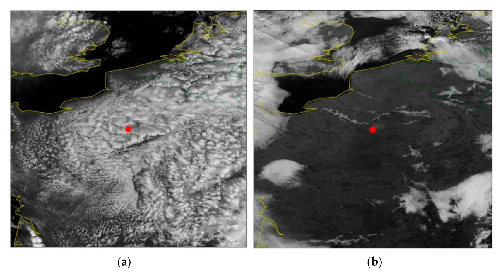
2.3.2. Satellite Data

SEVIRI is a 12-channel imager on the MSG geostationary satellites operated by EUMETSAT. In this work, we used the observations acquired from 01 July 2017 to 30 June 2020 mainly from MSG-3 and MSG-4 and punctually from MSG-1 when MSG-4 has been in maintenance. These data are delivered in real-time by the SATMOS service from Météo-France under the form of NetCDF files containing calibrated radiance. Images are continuously archived at Institut Pierre-Simon Laplace (IPSL) in Palaiseau.

The computation of CMV and the forecast algorithm uses the high-resolution visible channel (HRV) observing the Earth through a broadband from 0.4 to 1.1 µm. The spatial resolution of HRV data is 1 km at nadir, corresponding approximately to a pixel of 2 × 1.2 km² over Palaiseau (respectively, 3 km at nadir and 4 × 6 km² for infrared channels). The temporal resolution is 15 min for both channels.

MSG images are time stamped every 00, 15, 30 and 45 min of the hour. SEVIRI starts to scan the whole Earth disk at each time stamped instant. The scan duration is approximately of 12.5 min. Observation time of the pixel surrounding SIRTA observatory takes place 11 min after time stamped instant. Thus, cloud index can be derived at each 11, 26, 41 and 56 min of an hour.

2.3.3. ARPEGE Outputs

The NWP model ARPEGE is one of the operational forecast model used at Météo-France [48]. We use the output “surface solar radiation downwards” of ARPEGE, as a reference model to assess the satellite-based forecast. This model is operational as a global forecast system with a horizontal resolution of about 7.5 km over mainland France. Its initial conditions are determined by a 4D-Var data assimilation of observations. ARPEGE is a spectral hydrostatic model with a presentation in finite elements on the vertical direction. It presents 105 vertical levels from 10 m. to 75 km above sea level.

For each day, we selected the run initialized at 12:00 UTC for 0–24 h ahead with an hourly time resolution. Outputs have been linearly interpolated to coincide with MSG timestamps. Spatial resolution of this global model is 5 km over Europe.

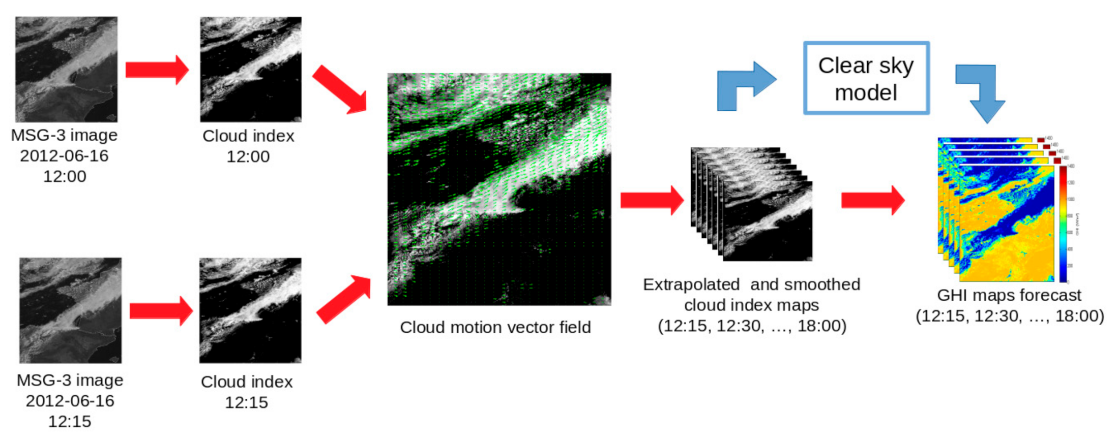
2.3.4. Cloud Index Computation

The conversion of HRV radiance into cloud index is made with an in-house version of the Heliosat method. This version is defined by the way to compute the different terms of the cloud index n defined in [33] and [31] by (3):

$$n=\frac{\rho -{\rho }_g}{{\rho }_c-{\rho }_g}$$

(3)

ρ is the reflectance derived from the calibrated radiance L observed by the sensor through the following equation:

$$\rho =\frac{\pi L{d}^2}{I_0\cos \theta }$$

(4)

where L is the calibrated radiance observed by the sensor, d is the Earth–Sun distance in AU temporally corrected by the Earth orbit eccentricity, I₀ is the total solar irradiance for the HRV channel and θ is the solar zenith angle (SZA) above the given pixel. ρ_c is the maximum observable reflectance assuming that it is due to the brightest cloud. According to [34], we determine ρ_c by the 95th percentile of all reflection values at local noon in the target region. We set this value to 78% for the whole studied period. Sensor change between MSG-1, -3 and -4 did not impact significantly this 95th percentile value. ρ_g is the ground albedo, typically the albedo of a pixel if the sky is cloud free. This is usually the relative minimum of the reflections during a certain time span (e.g., a month) derived for each pixel of the satellite image. In order to prepare our algorithm for operational application, we undertook an internal study, using almost 5 years of data, leading to the best GHI retrieval results with minimal operational constraints. Then, ρ_g was computed as the 4th percentile of all reflection values at a given time slot for a given month during the two years preceding a given month. The 4th percentile value has been selected as a good compromise to obtain ρ_g minimum values, avoiding secondary minimums and outliers. For example, for a GHI estimation from an MSG image acquired on any day of September 2020 at 12:00 UTC, ρ_g is the 4th percentile for all ρ values observed at 12:00 UTC during September 2018 and 2019. The retrievals are limited to θ less than 78°.

2.3.5. Cloud Motion Vector Field Computation

The algorithm computing cloud motion vector is detailed in [49]. It has been originally conceived to extract atmospheric motion vectors used as inputs of operational weather forecast models. Instead of using cloud index images as shown in Figure 2, this CMV computation method uses radiances. The process includes two main steps:

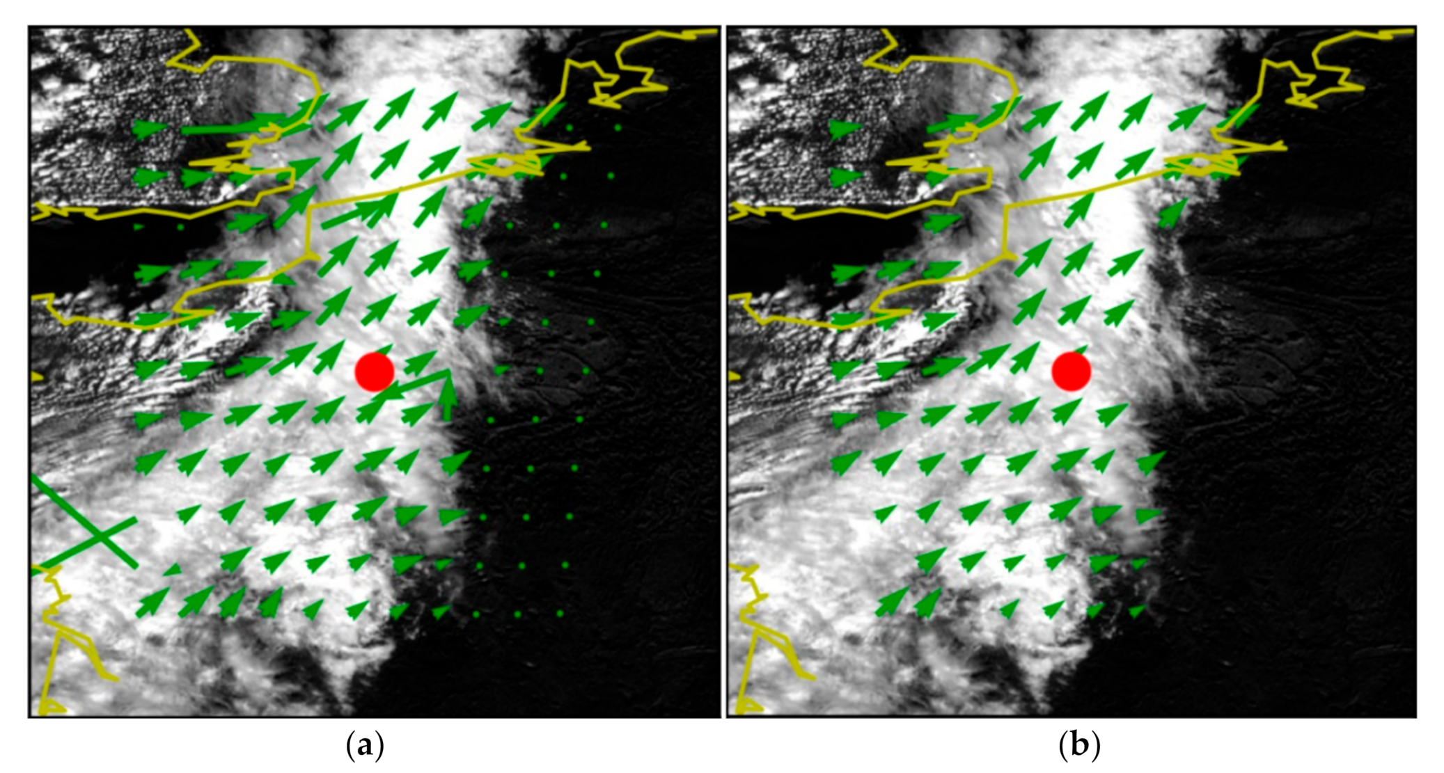
• In the first step, a CMV field is produced with a block-matching method based on the minimization of the sum of squared differences (SSD, or Euclidean distance) of pixel values (radiances). For each vector, if the forecast is initiated at time T0, a square of 36 × 36 pixels—called target window—is selected on the image acquired at T0-15 min (image 1). A square of 96× 96 pixels—the search window—is then selected in the image acquired at T0 (image 2) with the same center as the target window of image 1. The target window of image 1 is displaced pixel-by-pixel in all directions, over all possible positions allowed inside the search window of image 2. The relative position of the two windows presenting the minimal SSD is marked as the motion vector tip, and thus defines the CMV. In practice this process is applied to all the predefined positions of a regular grid and produces a CMV vector field between T0-15 min and T0. In this study we do not take into account the height (or level) of the tracked clouds. The resulting CMV fields may be composed of vectors at different levels. When clouds are present in different, overlapping layers, the satellite generally “sees” the clouds of the uppermost layer in the visible channel.
• A second CMV field has to be calculated over the same grid with the previously described procedure between the image acquired at T0-30 min (image 0) and the image acquired at T0-15 min (image 1), in order to detect unrealistic temporal evolution of the tracked cloud or structure during the half-hour period before T0, the forecast time, by comparing both vector fields. In practice, this second CMV field is extracted before the one derived between T0-15 min and T0).

Particularly in a heterogeneous cloud field, this process can lead to spatial incoherence between neighboring vectors or unrealistic directions or speed variations for some vectors. Thus, a series of quality tests is applied as a second step with the following criteria:

• Suppression of null vectors (corresponding often to cloud free areas).
• Suppression of vectors with a norm exceeding a realistic wind speed.
• Temporal consistency test: each vector calculated between T0-15 min and T0 is compared to its predecessor computed at the same location in the images acquired at T0-30 min and T0-15 min. If the difference in vector direction or the ratio of magnitude (proportional to the wind speed) of both vectors, exceed fixed thresholds, the vector is suppressed.
• Spatial consistency test: each vector is compared with its nearest neighbors. Similarly, if the difference in direction or the magnitude ratio exceeds fixed thresholds, the vector is suppressed.

In practice, the trackable clouds almost always stay at the same level over 1/4 h, the period between two consecutive satellite images used for CMV calculation. This may not be the case in the following situations:

• When clouds appear or dissipate (inside the area covered by the target window), they are only present on one image of a pair.
• Sometimes two clouds or cloud groups (or more) can be present at different levels inside a target window and can move at a different speeds or in different directions. The derived CMV may correspond to the motion of one of the clouds (generally the largest one, or in some cases the thickest cloud when semi-transparent clouds (cirrus) are also present. Or the CMV may correspond to some “mixture” of the motion of both clouds.

In both situations the resulting vector generally shows important differences in speed and/or direction with its neighbors, and/or with its collocated predecessor or successor, and therefore will be suppressed by quality tests, mainly by temporal and spatial consistency tests.

In the current implementation, a CMV is computed over an area of 513 × 513 pixels centered on Palaiseau. A vector is computed every 36 pixels. Figure 3 shows an example of computed CMV before and after the consistency tests. It can be seen that the consistency tests suppressed two very long vectors near the south-west corner of the image.

2.3.6. Cloud Index Image Extrapolation and Post-Processing

At a forecast initiation time T0, once the cloud index and the CMV have been computed, the latter is applied on the cloud index derived from the satellite image acquired at T0 for its extrapolation. Every pixel included in the 36 × 36 pixels block containing a vector is shifted according to its norm and direction. Thus, the cloud index values stay the same, while their position can change.

The extrapolation is made for every time horizon h from 15 to 360 min with a 15 min time step. The extrapolation is made “step-by-step”: the cloud index map forecast at time horizon h is the result of the extrapolation applied on the forecast result of h-15 min. This allows taking into account a smoother cloud motion, in particular for a rotating motion. Indeed, a “direct” extrapolation of the image T0 to every time horizon steps lead to a homothetic shape of the original image, ignoring the curved motions. This process enables us to obtain, at time T0, a time-series of 24 extrapolated images up to h = 6 h.

Numerous authors, including [36], apply a smoothing filter on extrapolated images. This permits a reduction in forecast errors by eliminating small randomly varying structures that can become unrealistic after the extrapolation process. However, if it reduces the errors in term of hourly energy sums, the results lead to a reduction in GHI variability [39]. If a low error rate in the hourly energy sum is better for applications such as electricity trading, forecasting the actual variability can be useful for micro-grid applications, where forecasting the ramp-rates accurately is more fruitful than forecasting the PV power magnitude. In the present study, we applied a rectangular low-pass filter with size increasing with time-horizon.

2.3.7. Forecast GHI Computation

The last step of the forecast algorithm is the conversion of the target pixels into GHI values. We extracted the pixel including the site of Palaiseau and computed the clear-sky index Kc from the cloud index value, following the relationship given by [34]. Thus, the generic simplified Equation (1) became:

$$K_c=\left\{\begin{array}{c}1.2\mathrm{for}n⩽-0.2\\ 1-n\mathrm{for}-0.2 \text{<}n⩽0.8\\ 1.661-17.781n+0.73n^2\mathrm{for}0.8\text{<}n⩽1.05\\ 0.09\mathrm{for}n\text{>}1.05\end{array}\right\}$$

(5)

For computing GHI_cs, we selected the clear-sky model called SOLIS [50,51] available through the pvlib library [52]. To simplify the implementation of our forecast algorithm, we use the monthly climatological means of aerosol optical depth proposed in this library and assigned a constant value for water vapor concentration. SOLIS has been widely used and tested as a robust model with a stable accuracy even with climatological data such as aerosols inputs [53]. The forecast values of K_c = K_c (T₀ + h) are finally converted into GHI (T₀ + h) using (2).

3. Forecast Predictors

Solar irradiance variability is driven by its two mains components:

• The deterministic variability only dependent on the course of the Sun, directly and entirely quantified by the solar zenith angle θ.
• The stochastic variability of cloud cover, depending on the weather situation at multiple spatio-temporal scales. Thus, its quantification can be made through various parameters influencing cloudiness at the intra-day scale.

For cloud cover variability, we limited the study to three potential predictors: the observed clear sky index on the punctual site, the clear sky index map surrounding the SIRTA site and the weather regimes occurring in the northern Atlantic and western Europe. These parameters are likely to present links with the intraday irradiance variability at the kilometric scale. Moreover, their observation and forecast are available even for operational conditions. Thus, they can be used to predict the expected uncertainty of operational forecasts.

3.1. Predictor Solar Zenith Angle

The SZA variation describes the daily and seasonal course of the Sun. It determines the maximum possible irradiance for a given instant and also influences the magnitudes of forecast errors. Moreover, GHI retrieval from satellite images at high SZA values (when the Sun appears close to the horizon) induces higher error rates, mainly due to possible misalignment of cloud and its shadow viewed from the satellite, as well as an overestimation of reflectance computed in (4) leading to false cloud detection (overestimation of cloud index). SZA values are computed through the Solar Position Algorithm (SPA) [54] also available in pvlib [52].

3.2. “Observed” Clear-Sky Index

What is denoted here by “observed” clear sky index is the value of K_{c_obs}, computed with the measured GHI_obs from pyranometer:

$$K_{c\_obs}=\frac{GH{I}_{obs}}{GH{I}_{cs}}$$

(6)

GHI_obs and GHI_cs are both available at forecast initialized time if the site is equipped with a pyranometer. Values of K_{c_obs} at this instant assume to represent the possible state of the sky. For extreme values, the sky is overcast or cloud free meaning a relative stability at least in the first tens of minutes. For intermediate values, the sky is often covered by a heterogeneous cloud field that can change quickly.

3.3. Spatial Pattern of Surrounding Clear-Sky Indices Assessed from Satellite

K_{c_obs} is observable only from the punctual target site, delivering information on surrounding situation only through assumptions. As computation of cloud indices of the whole studied area of the satellite image is a necessary step for the extrapolation process (see Section 2.3.5), the clear-sky indices over the surrounding area of the target site are easy to obtain.

We consider the clear indices map of 7 × 7 MSG-HRV pixels, representing approximately a rectangle of 8 × 14 km² surrounding Palaiseau. From this map at each forecast initialization instant, we computed the arithmetic mean of the 49 clear-sky indices assessed from satellite image and their standard deviation. These two parameters enable us to quantify the magnitude of the cloudiness and its spatial distribution inside this surrounding area.

3.4. Weather Regimes of North Atlantic-Europe Domain

Cloudiness patterns and their spatiotemporal evolution originate from weather characteristics at larger synoptic scales (pressure and temperature fields). For the northern Atlantic area, four situations per season have been identified as distinct weather regimes [55,56]. The impacts of each weather regime on the meteorological situation in Paris area have been studied by [28,57], who investigated the influence of these same weather regimes on solar and wind energy production.

Weather regimes are distinguished by clustering the daily maps of anomalous 500 hPa geopotential height in the north Atlantic–European region. The classification of Cassou [58] presents four different cases:

• An anticyclone over northern Canada and Greenland and a zonal circulation towards Europe: this regime corresponds to the negative value of the Northern Atlantic Oscillation (NAO) and it is therefore called NAO−.
• An anticyclone in the middle of the Atlantic. This regime is called the Atlantic Ridge.
• An anticyclone over the North Sea: Scandinavian Blocking.
• A depression over Iceland in winter and a pronounced zonal circulation toward Europe in summer. This regime corresponds to the positive phase of the NAO (or NAO+). It is called the Atlantic Low in winter and Zonal in summer.

Van Der Wiel et al. [57] focused on winter situations, whereas [28] studied summer situations only. From these two works we deduced the expected consequences on the cloud cover evolution over the Paris area. For both summer and winter, cold and wet circulation are more often brought by NAO− and the Atlantic Ridge, whereas dry and warm fluxes are rather caused by Scandinavian Blocking and NAO+ regimes.

To verify these assumptions, we computed average hourly GHI measurements, observed by pyranometers for various regimes. We obtained the regime daily classification from [59], which does not guarantee the results for spring and autumn. Therefore, in the rest of this present paper, all presented results according to weather regimes will concern only summer defined by June, July and August and winter (December, January, and February). Results are summarized in

Table 1. Average ground measurements (Baseline Surface Radiation Network—BSRN Palaiseau) of GHI from July 2017 to June 2020 distinctly for summer (DJF) and winter (JJA). Measurements when solar zenith angle (SZA) is superior to 78° have been excluded. NAO: Northern Atlantic Oscillation.

Season	Weather Regime	GHI Mean (Wm−2)	Number of Observations
Summer	All regimes	455	12,837
	NAO−	454	3139
	Atlantic Ridge	421	3642
	Scandinavian Blocking	490	2985
	Zonal (NAO+)	467	3071
Winter	All regimes	176	5988
	NAO−	183	455
	Atlantic Ridge	135	1635
	Scandinavian Blocking	215	1555
	Atlantic low (NAO+)	178	2343

. We remark that this assumption is verified in summer but with small differences. Scandinavian Blocking and zonal regimes show higher GHI values. In winter, significantly low occurrences of the NAO− regime affect the statistical quality of the results. However, Scandinavian Blocking presents a net superiority in averaged irradiance in winter compared to the other regimes.

For a deeper vision of weather regimes’ impact on cloud cover observed by satellites, we manually visualized the MSG images of the same periods classified in these four regimes. We deduced some trends showing that NAO+ and NAO− present, most of the time, a uniform advection of the cloud field in the considered area. Atlantic Ridge presented a majority of convection cases and Scandinavian Blocking showed large cloud free areas. Figure 4 shows representative images of Atlantic Ridge and Scandinavian Blocking corresponding to our first assumptions. We assumed that these trends and the image representativeness are based on our subjective considerations.

4. Results

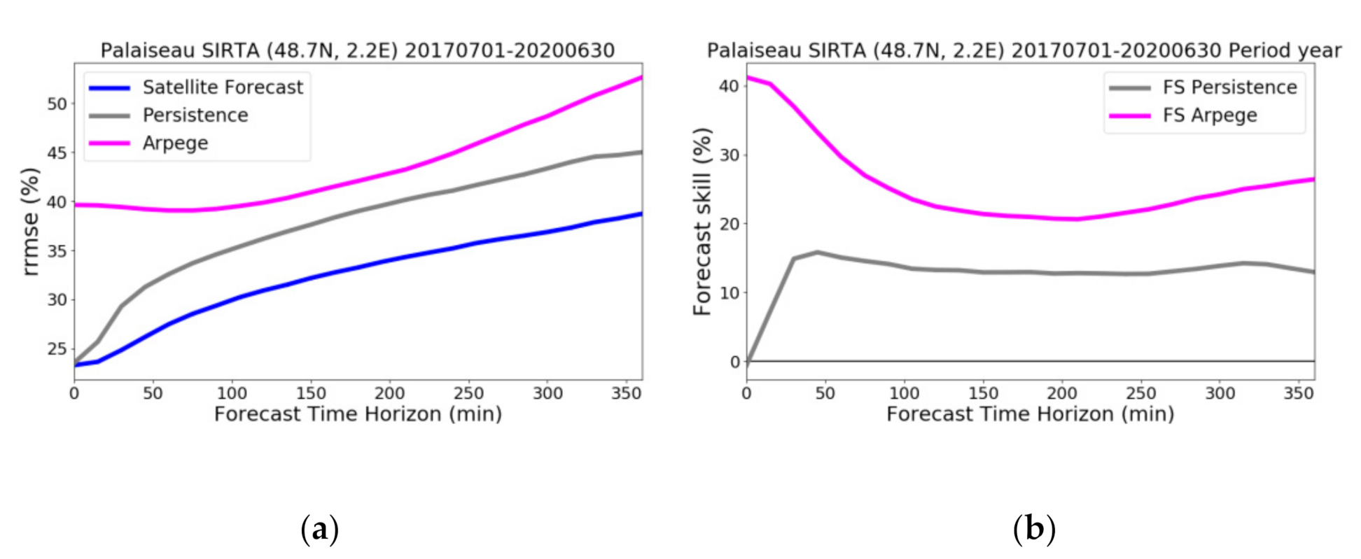
4.1. Evaluation Protocol

The GHI forecasts for the single pixel colocated at Palaiseau are compared with the GHI measured by the BSRN station. In order to compare instant pixelwise value from satellites with local ground measurements, we converted both satellite and ground data irradiation sums to 15 min time steps irradiation sums. Then, for a given satellite acquisition time (e.g., 12.11 UTC), we compared both irradiations summed over the last 15 min from 11.57 UTC to 12.11 UTC. Minute resolution ground data have been simply summed over these 15 min. For satellite data, we first computed a GHI forecast value at each minute between the two acquisitions using a temporal linear interpolation between 11.57 and 12.11 UTC of predicted clear-sky index. Then we computed the GHI every minute, given that the clear sky model is able to provide GHI_cs value at 1 min steps. Then forecast data have been summed over these 15 min. This protocol follows the recommendations of [60] who advise to take into account the Sun position at each minute to synthesize the 15 min information gap due to satellite sensor resolution.

We performed the forecast using all HRV images available at IPSL from 1 July 2017 to 30 June 2020. We only used images sufficiently illuminated by the Sun to compute CMV and cloud index maps. We rejected all data computed with an SZA above 78°. In practice, the first and last daily observations used in July were time stamped at 5.26 and 18.26 UTC. In January, forecasts started at 9.41 and ended at 14.11 UTC.

4.2. General Results

We computed errors between all forecast (GHI_for) and observation (GHI_for) values by classifying them in time horizon from 0 to 360 min with 15 min time step. We use the mean bias error (MBE), mean absolute error, RMSE and correlation coefficient or Pearson coefficient (R), respectively, defined by (7), (8), (9) and (10).

$$MBE=\frac{1}{N}{\displaystyle \sum }_{i=1}^N\left(GH{I}_{for,i}-GH{I}_{obs,i}\right)$$

(7)

$$MAE=\frac{1}{N}{\displaystyle \sum }_{i=1}^N\left|GH{I}_{for,i}-GH{I}_{obs,i}\right|$$

(8)

$$RMSE=\frac{1}{N}{\displaystyle \sum }_{i=1}^N\sqrt{{\left(GH{I}_{for,i}-GH{I}_{obs,i}\right)}^2}$$

(9)

$$R=\frac{Cov\left(GH{I}_{for},GH{I}_{obs}\right)}{{\sigma }_{GH{I}_{for}}*{\sigma }_{GH{I}_{obs}}}$$

(10)

where Cov (GHI_for,GHI_obs) is the covariance between forecast and observation values ; σ_GHIfor and σ_GHIobs are standard deviations of, respectively, forecast and observation values.

Table 2. Statistics of GHI satellite-based forecast at Palaiseau from 1 July 2017 to 30 June 2020.

Forecast Horizon (min)	Observation Mean Wm−2	Mean Bias Error W.m−2 (%)	Mean Absolute Error Wm−2 (%)	Root Mean Square Error Wm−2 (%)	Correlation Coefficient	Observation Number
0	364	−17 (−5)	57 (16)	85 (23)	0.94	36,541
15	364	−16 (−4)	58 (16)	86 (24)	0.94	36,327
60	382	−16 (−4)	70 (18)	105 (27)	0.91	33,473
120	408	−18 (−4)	87 (21)	126 (31)	0.87	29,131
180	425	−18 (−4)	99 (23)	141 (33)	0.84	25,043
240	431	−17 (−4)	107 (25)	152 (35)	0.83	25,043
360	420	−11 (−2)	115 (27)	163 (39)	0.78	14,067

shows the results of several metrics for selected typical time horizons. Relative value corresponds to the absolute value divided by mean of GHI ground measurements. Results at time horizon of 0 min evaluate our algorithm of GHI estimation from satellite. Results are similar to the state-of-the-art for Palaiseau station. In particular, [60] published very close results in terms of relative RMSE (25.5% and 24.8% for the GHI database HelioClim-3 version 4 and version 5, respectively). The high value of the correlation coefficient ensures consistent results.

Error metrics increase with time horizon except for bias error. However, results are satisfactory in the magnitude of order from similar works using ground truth data in the Netherlands [21] and Germany [43] at different periods. Figure 5a shows the RMSE results compared with those of ARPEGE model and persistence algorithm as reference algorithms. The persistence algorithm generally used in the intraday algorithm consists in considering that clear-sky index K_c value is constant from forecast initialization time T0 to time horizon h (9). In other words, this naive algorithm takes into account the course of the Sun but assumes that cloud cover did not change at all during the forecast.

$$K_c\left(T_0+h\right)= K_c\left(T_0\right)$$

(11)

Figure 5b presents the same results under the form of the forecast skill (FS), which compares the RMSE of the forecast algorithm (RMSE_for) to the one of a reference model (RMSE_ref) which is either the persistence (grey curve) and ARPEGE (magenta curve) computed with Formula (12). A positive value of FS means that RMSE_for is lower than RMSE_ref.

$$\mathrm{FS}=\left(1-\frac{RMS{E}_{for}}{RMS{E}_{ref}}\right)$$

(12)

It highlights the evidence that satellite-based forecast present smaller errors than an NWP at these time horizons. Moreover, the persistence algorithm presents larger errors. The difference of errors between forecast and persistence increases with the time horizon.

Figure 6 shows the forecast skills according to the four seasons defined as trimesters with complete months. The skill scores have similar layouts except for wintertime mainly due to shorter daytime and thus, are less statistically representative. For all seasons, the satellite forecast gives better results than the NWP forecast and persistence. The overall results show a satisfactory consistence regarding the state-of-the-art and enable to investigate forecast uncertainty sensitivity to the selected predictors.

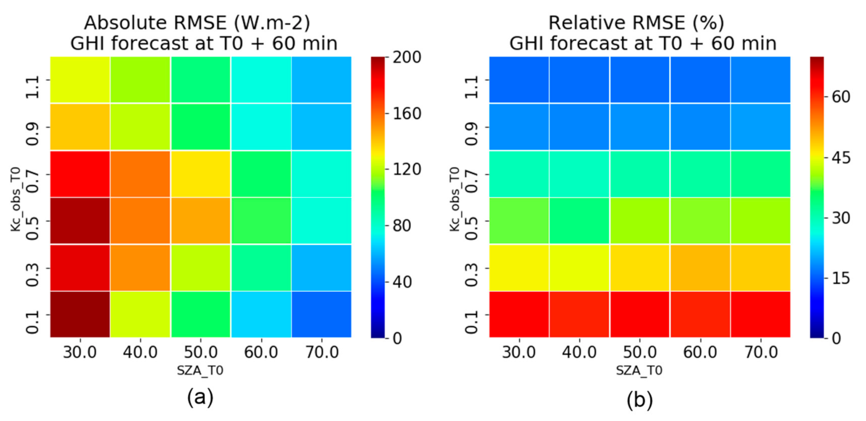
4.3. Results against Punctual Predictors

Local predictors, namely the SZA and the observed clear-sky, have their values defined at forecast target point and at forecast initialization time T0. For commodity, we present the RMSE results as a function of both predictors. Figure 7 shows so-called “heatmaps” of the absolute (a) and relative RMSE (b) of the forecast for all seasons at a time horizon of 60 min.

Such figures show that the Sun at its highest position with an intermediate state of cloud cover clearly affects the absolute RMSE. When the magnitude of GHI is higher with a lower SZA value, the absolute error increases. As mentioned previously in Section 3.2, intermediate values of K_{c obs} occur when the cloud cover is not homogeneous and when it can evolve rapidly. The relative RMSE is more regularly sensitive to the K_{c obs} and is impacted by the lowest Sun elevations. As this metric is weighted with the mean of the observation values, the Sun position effect is strongly attenuated and the errors appear larger for low GHI values. Heatmaps from other time horizons (not shown) present similar patterns. Similar results have been highlighted for the NWP-based forecast in [25]. Such information is relevant at least for network managers dealing with large PV farms. A variation of absolute errors can induce a large difference in terms of PV electricity resource for grid dispatching.

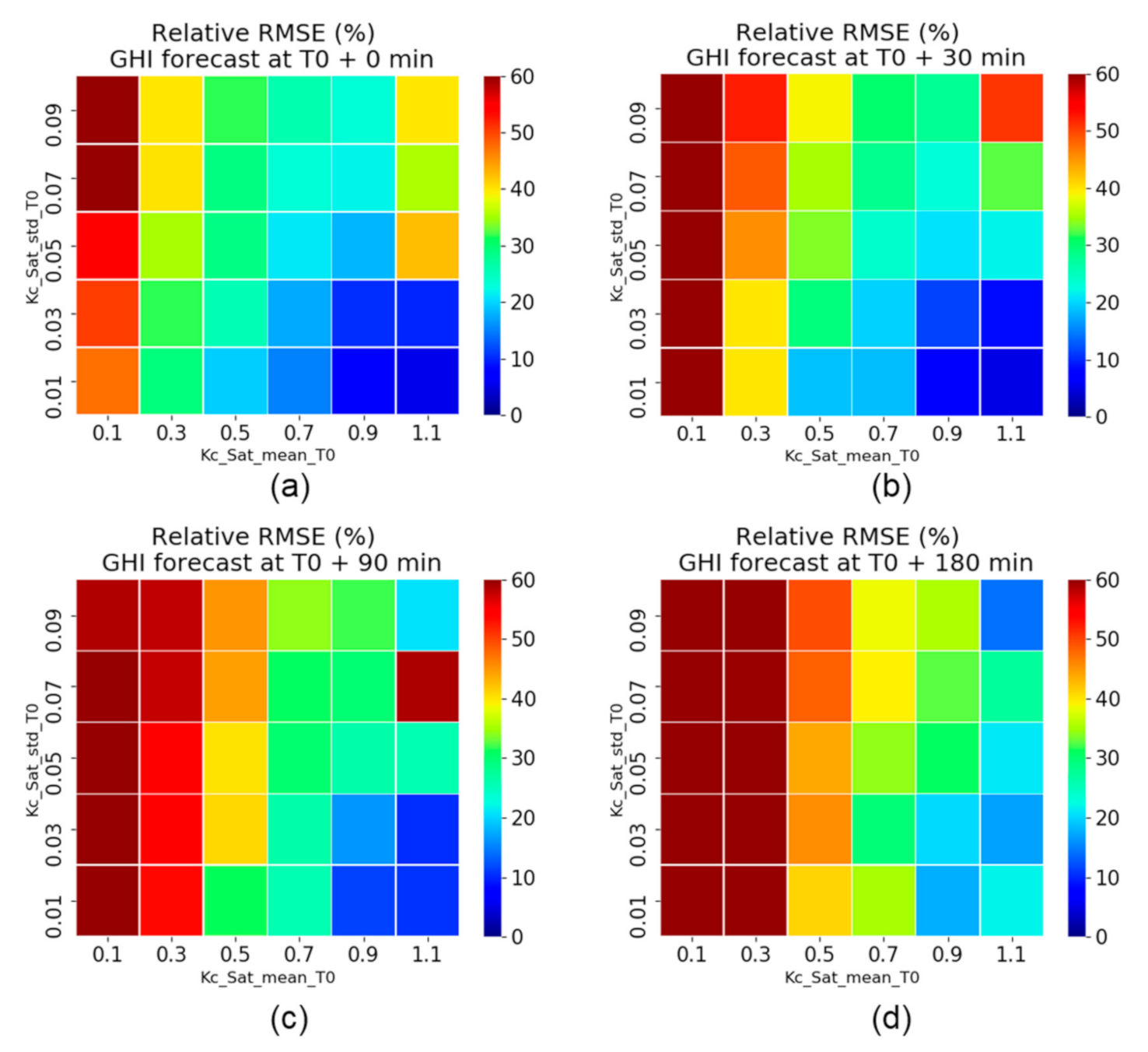
4.4. Results against Neighboring Clear-Sky Index Pattern Observed by Satellite

Figure 8 shows the relative RMSE as a function of the mean and the standard deviation of surrounding K_c as described in Section 4.3. It shows a clear evolution of error pattern according to the time horizon. At T0 + 0 min, we can notice that for any classes of K_c, the error increases with the standard deviation. This is more pronounced for extreme values of the means of K_c. Indeed, cases of overcast or clear sky induce large errors if spatial heterogeneity increases.

For later time horizons, the relative RMSE becomes larger for lowest values of K_c but the increase with standard deviation is less pronounced. The errors for the clear-sky situation are more stable and quite low. Whatever the time horizon, the maps show an increasing variation of the errors with the spatial heterogeneity of the area.

These distinct signals, which are a function of time horizon, can be useful to predict the forecast error magnitude as a function of the current cloud cover neighboring pattern. Further studies could be done by choosing different sizes of the neighboring area in order to refine this error prediction.

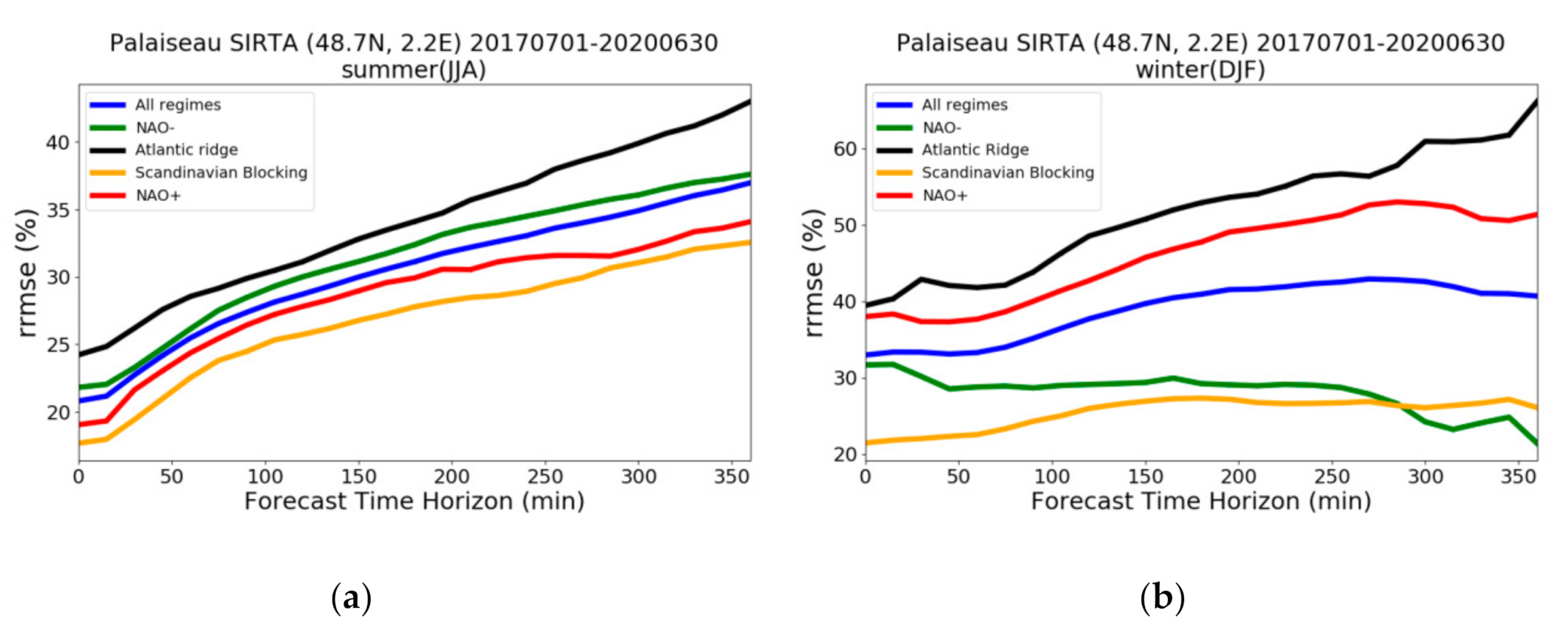
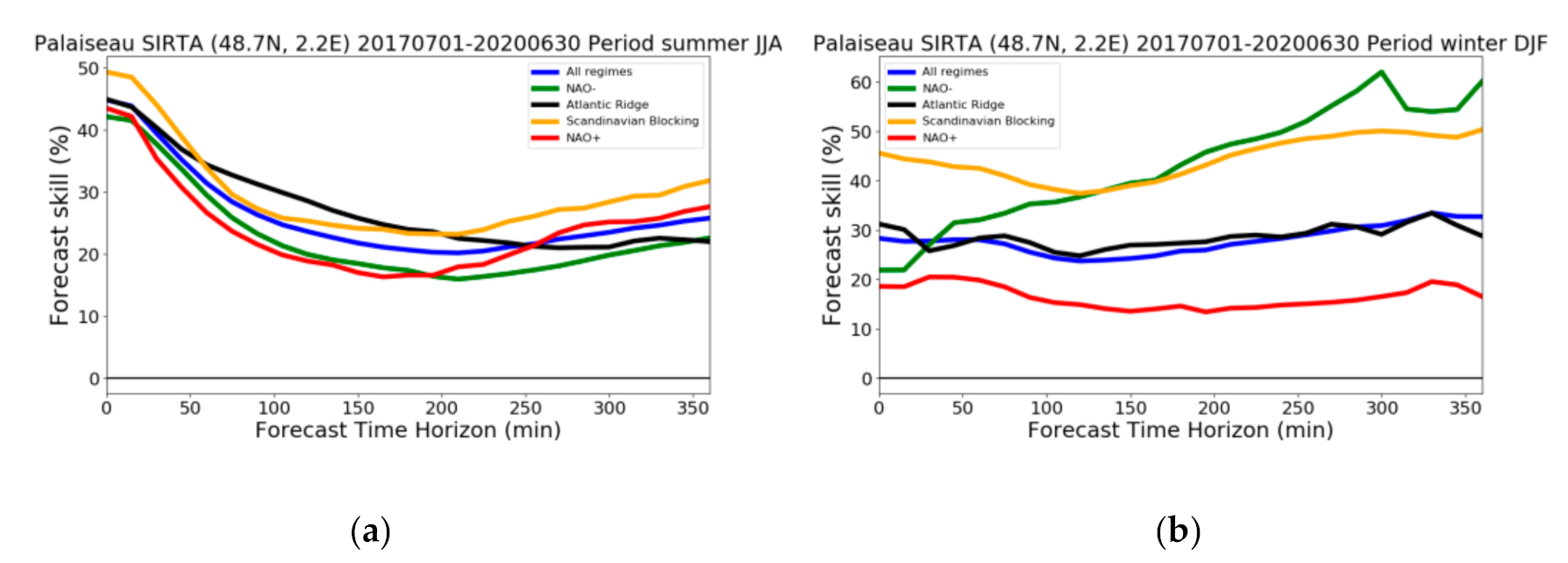
4.5. Results against Synoptic Weather Regimes

We plotted the relative RMSE of the satellite-based forecast according to the four weather regimes presented in Section 3.4. Figure 9 shows the curve as a function of the time horizon. The blue curve labeled “All regimes” gathers all the forecast whatever the weather regime and is plotted here as a reference. The other curves show the RMSE of forecast occurring during the considered weather regimes. A weather regime occurrence is attributed on a daily basis. Therefore, any forecast starts and ends within the same weather regime. The results show a clear distinction of the error according to each weather regime, even between the two considered seasons.

In summer, the relative RMSE according to regime presents a constant ranking for all time horizons. The Atlantic Ridge presents the largest errors. Relative RMSE increases from 4% to 6% compared to all situations. Scandinavian Blocking shows a significantly lower error (−5% to −4%) than the other regimes. NAO+ and Zonal (NAO−) remain close to the general score of the forecast. However, NAO−shows a relative RMSE up to 5% larger than NAO+.

In winter, relative RMSE is significantly higher than in summer. Colder temperatures and humidity lead to more frequent cloudy situations where this type of forecast is less accurate as mentioned, for example, by [21]. Moreover, shorter daytime duration decreases the observation number compared to summer, which increases the relative RMSE. Winter results show an inverted ranking concerning weather regimes defined by the NAO. NAO+ appears much less accurate than all regimes, whereas Atlantic Low (NAO−) shows a smaller error. However, the divergent results of NAO− in winter is also explained by the weak number of occurrences of this regime as noticed in Table 1. Scandinavian Blocking decreases the relative RMSE from 11% to 14% when the Atlantic Ridge increases it from 7% to 16%.

For both seasons, the performances under the Atlantic Ridge and Scandinavian Blocking regimes follow the magnitude of the GHI estimation presented in Table 1. It provides a loss of 4% to 5% in relative RMSE. The Atlantic Ridge increases the RMSE by 4%–6%. In winter, these respective variations are 11%–14% and 7%–16%.

Thus, this forecast error ranking can be explained by the relative warmer and drier situation in Europe due to the proximity of anticyclonic situations during the Scandinavian Blocking regime. The cold and humid conditions of the Atlantic Ridge induced more depressions and unstable cloudy situations, which affected the forecast accuracy. These results for these two regimes are consistent with the satellite image example presented in Figure 4.

Such a clear ranking is a useful result because weather regime occurrences can be forecast accurately several days in advance through NWP models and therefore predict the magnitude of intraday error forecast.

Figure 10 shows the forecast skill of satellite-based forecast against those of ARPEGE. We can remark that the performances according to weather regime do not show the same ranking as for relative RMSE. In summer, the Atlantic Ridge and Scandinavian Blocking regimes have the highest skill scores up 250 min of time horizon. We can deduce that during the Atlantic Ridge regime, the forecast is less accurate even for ARPEGE. The NAO+ and NAO−regimes present the worst forecast skill score meaning that even if satellite forecasts present better results than NWP at these time horizons, forecasting GHI during the two NAO phases seems to give better results for ARPEGE compared to other weather regimes.

In winter, unsurprisingly, the Scandinavian Blocking regime shows the best score. NAO+ presents the worst score, confirming the better skill for ARPEGE to forecast GHI during such regime. However, this result does not concern NAO−, certainly due to its lack of occurrence.

5. Conclusions

This work is aimed at identifying relationships between the accuracy of an intraday surface solar irradiance forecast method and meteorological variables that can be easily observed or forecast. Firstly, we proposed an irradiance forecast method using satellite images, based on general principles already known from the recent state-of-the-art. Similar methods have been used on operational and commercial bases for several years. We tested herein the implementation of a proven cloud motion vector computation method, routinely used to extract wind vectors in operational conditions. Secondly, we proposed a long-term validation over three complete years using ground measurements and a comparison with an NWP model (ARPEGE). The results showed forecast errors varying with time horizon from 24% at 15 min to 39% at 6 h in relative RMSE (corresponding, respectively, to 86 and 163 Wm⁻² in RMSE). Whatever the forecast horizon, the method shows a positive forecast skill score compared to persistence (up to 15%) and ARPEGE model (between 20% and 40%). The bias is almost constant about–17 Wm⁻² (5% in relative value) whatever the time horizon. Even if this validation is restricted to one location, the good results regarding the state-of-the-art methods enable further studies on the uncertainties.

Finally, we evaluate the accuracy sensitivity with respect to meteorological conditions quantified by the Sun’s elevation, the cloud cover pattern surrounding the target site and the synoptic weather regimes. We showed, for example that, according to clear-sky index spatial distribution at forecast initialization time, the relative RMSE at 90 min may vary from less than 15% for a clear-sky condition to more than 50% for heterogeneous cloudy skies. A weather regime occurrence can be known several days in advance. It is found that the summer Scandinavian Blocking regime is related to the lowest relative RMSE, whereas the Atlantic Ridge regime shows the highest errors. The difference of relative RMSE between these two regimes is from 8% to 10% in summer according to time horizon. In winter, this difference is much higher, from 18% at the earliest time horizon steps to 30% after 5 h. These results confirm the lower accuracy of this forecast method in the case of heterogeneous cloud cover as observed using clear-sky index spatial distribution heatmaps. Such a situation often occurs often during the Atlantic Ridge regime. The extrapolation of a cloud cover using only a CMV constant in time during the forecast induces larger errors when the cloud cover strongly varies in space and time.

Our results permit to propose these predictors to solar energy forecast users. These predictors can be either known when the forecast starts or several days in advance (which is the case of weather regimes). This enables us to anticipate the reliability of an intraday forecast using a CMV-type technique. It can be particularly useful for micro-grid applications where the energy management methods to optimize PV electricity consumption with forecast are part of a growing experimental field over the world [61].

These predictors have been selected for their known influence of the uncertainty of solar irradiance estimation using satellite data. However, this predictor list is certainly not exhaustive and further parameters can be tested, in particular, if the latter are easy and cheap to obtain in operational conditions. A key result of our work is the highlighted dependence between forecast accuracy and weather regimes occurring in the Paris area. Such work can be of course tested on different areas influenced by identified weather regimes. Moreover, deeper studies on synoptic barometric fields may provide additional predictors derivable from available meteorological observations.

Finally, this methodology can also be undertaken for other types of solar irradiance forecast algorithms because weather regime occurrence has direct influence on cloud cover behavior. More and more developing forecast methods include a machine-learning approach. Identified predictors could be used as pertinent inputs to improve their results.

References

1. Morjaria, M.; Anichkov, D.; Chadliev, V.; Soni, S. A Grid-Friendly Plant: The Role of Utility-Scale Photovoltaic Plants in Grid Stability and Reliability. IEEE Power Energy Mag. 2014, 12, 87–95. [Google Scholar] [CrossRef]
2. International Renewable Energy Agency. Renewable Capacity Statistics; International Renewable Energy Agency: Abu Dhabi, UAE, 2020. [Google Scholar]
3. Golestaneh, F.; Pinson, P.; Gooi, H.B. Very Short-Term Nonparametric Probabilistic Forecasting of Renewable Energy Generation—With Application to Solar Energy. IEEE Trans. Power Syst. 2016, 31, 3850–3863. [Google Scholar] [CrossRef] [Green Version]
4. Calderon-Olbadia, F. Photovoltaic Power Generation Uncertainty Forecast for Microgrid Energy Management Efficiency Enhancement. Ph.D. Thesis, Université Paris-Sud, Paris, France, 2020. [Google Scholar]
5. Perez, M.; Perez, R.; Rábago, K.R.; Putnam, M. Overbuilding & curtailment: The cost-effective enablers of firm PV generation. Sol. Energy 2019, 180, 412–422. [Google Scholar]
6. Ocker, F.; Jaenisch, V. The way towards European electricity intraday auctions—Status quo and future developments. Energy Policy 2020, 145, 111731. [Google Scholar] [CrossRef]
7. Helbig, N. Application of the Radiosity Approach to the Radiation Balance in Complex Terrain. Dr. Thesis, University of Zurich, Zurich, Switzerland, 2009. [Google Scholar]
8. Dobos, A.P. PV Watts Version 5 Manual (No. NREL/TP-6A20-62641); National Renewable Energy Lab: Golden, CO, USA, 2014. [Google Scholar]
9. Diagne, H.M.; David, M.; Lauret, P.; Boland, J.; Schmutz, N. Review of solar irradiance forecasting methods and a proposition for small-scale insular grids. Renew. Sustain. Energy Rev. 2013, 27, 65–76. [Google Scholar] [CrossRef] [Green Version]
10. Antonanzas, J.; Osorio, N.; Escobar, R.; Urraca, R.; Martinez-De-Pison, F.; Antonanzas-Torres, F. Review of photovoltaic power forecasting. Sol. Energy 2016, 136, 78–111. [Google Scholar] [CrossRef]
11. Barbieri, F.; Rajakaruna, S.; Ghosh, A. Very short-term photovoltaic power forecasting with cloud modeling: A review. Sustain. Energy Rev. 2017, 75, 242–263. [Google Scholar] [CrossRef] [Green Version]
12. Sobri, S.; Koohi-Kamali, S.; Rahim, N.A. Solar photovoltaic generation forecasting methods: A review. Energy Convers. Manag. 2018, 156, 459–497. [Google Scholar] [CrossRef]
13. Ahmed, R.; Sreeram, V.; Mishra, Y.; Arif, M. A review and evaluation of the state-of-the-art in PV solar power forecasting: Techniques and optimization. Renew. Sustain. Energy Rev. 2020, 124, 109792. [Google Scholar] [CrossRef]
14. Voyant, C.; Notton, G.; Kalogirou, S.; Nivet, M.-L.; Paoli, C.; Motte, F.; Fouilloy, A. Machine learning methods for solar radiation forecasting: A review. Renew. Energy 2017, 105, 569–582. [Google Scholar] [CrossRef]
15. Jang, H.S.; Bae, K.Y.; Park, H.-S.; Sung, D.K. Solar Power Prediction Based on Satellite Images and Support Vector Machine. IEEE Trans. Sustain. Energy 2016, 7, 1255–1263. [Google Scholar] [CrossRef]
16. Vandeventer, W.; Jamei, E.; Thirunavukkarasu, G.S.; Seyedmahmoudian, M.; Soon, T.K.; Horan, B.; Mekhilef, S.; Stojcevski, A. Short-term PV power forecasting using hybrid GASVM technique. Renew. Energy 2019, 140, 367–379. [Google Scholar] [CrossRef]
17. Urbich, I.; Bendix, J.; Müller, R. A Novel Approach for the Short-Term Forecast of the Effective Cloud Albedo. Remote. Sens. 2018, 10, 955. [Google Scholar] [CrossRef] [Green Version]
18. Kurzrock, F.; Cros, S.; Ming, F.C.; Otkin, J.A.; Hutt, A.; Linguet, L.; Lajoie, G.; Potthast, R. A Review of the Use of Geostationary Satellite Observations in Regional-Scale Models for Short-term Cloud Forecasting. Meteorol. Z. 2018, 27, 277–298. [Google Scholar] [CrossRef]
19. Perez, R.; Kivalov, S.; Schlemmer, J.; Hemker, K.; Renné, D.; Hoff, T.E. Validation of short and medium term operational solar radiation forecasts in the USA. Sol. Energy 2010, 84, 2161–2172. [Google Scholar] [CrossRef]
20. Lorenz, E.; Kühnert, J.; Heinemann, D.; Nielsen, K.P.; Remund, J.; Müller, S.C.; Cros, S. Comparison of irradiance forecasts based on numerical weather prediction models with different spatio-temporal resolutions. In Proceedings of the 31st European PV Solar Energy Conference, Hamburg, Germany, 14–18 September 2015. [Google Scholar]
21. Wang, P.; van Westrhenen, R.; Meirink, J.F.; van der Veen, S.; Knap, W. Surface solar radiation forecasts by advecting cloud physical properties derived from Meteosat Second Generation observations. Sol. Energy 2019, 177, 47–58. [Google Scholar] [CrossRef]
22. Yang, D.; Killinger, S.; Lingfors, D.; Engerer, N. Improved satellite-derived PV power nowcasting using real-time power data from reference PV systems. Sol. Energy 2018, 168, 118–139. [Google Scholar]
23. Cros, S.; Turpin, M.; Lallemand, C.; Souchard de Lavoreille, H.; Kurzrock, F. Satellite-Based Cloud Cover Detection and Tracking for Solar Irradiance Forecasting, European Geosciences Union General Assembly; Geophysical Research Abstracts: Vienna, Austria, 2019; Volume 21, p. 14784. [Google Scholar]
24. Blanc, P.; Remund, J.; Vallance, L. Short-term solar power forecasting based on satellite images. In Renewable Energy Forecasting; Woodhead Publishing: Sawston, UK, 2017; pp. 179–198. [Google Scholar]
25. Sengupta, M.; Habte, A.; Kurtz, S.; Dobos, A.; Wilbert, S.; Lorenz, E.; Stoffel, T.; Renné, D.; Myers, D.; Wilcox, S.; et al. Best Practices Handbook for the Collection and use of Solar Resource Data for Solar Energy Applications; Technical report; NREL: Golden, CO, USA, 2015. [Google Scholar]
26. Driemel, A.; Augustine, J.; Behrens, K.; Colle, S.; Cox, C.; Cuevas, E.; Denn, F.M.; Duprat, T.; Fukuda, M.; Grobe, H.; et al. Baseline Surface Radiation Network (BSRN): structure and data description (1992–2017). Earth Syst. Sci. Data 2018, 10, 1491–1501. [Google Scholar] [CrossRef] [Green Version]
27. Haeffelin, M.; Barthes, L.; Bock, O.; Boitel, C.; Bony, S.; Bouniol, D.; Chepfer, H.; Chiriaco, M.; Cuesta, J.; Delanoe, J.; et al. SIRTA, a ground-based atmospheric observatory for cloud and aerosol research. Ann. Geophys. 2005, 23, 253–275. [Google Scholar] [CrossRef] [Green Version]
28. Ringard, J.; Chiriaco, M.; Bastin, S.; Habets, F. Recent trends in climate variability at the local scale using 40 years of observations: The case of the Paris region of France. Atmospheric Chem. Phys. Discuss. 2019, 19, 13129–13155. [Google Scholar] [CrossRef] [Green Version]
29. Tarpley, J.D. Estimating Incident Solar Radiation at the Surface from Geostationary Satellite Data. J. Appl. Meteorol. 1979, 18, 1172–1181. [Google Scholar] [CrossRef] [Green Version]
30. Cano, D.; Monget, J.; Albuisson, M.; Guillard, H.; Regas, N.; Wald, L. A method for the determination of the global solar radiation from meteorological satellite data. Sol. Energy 1986, 37, 31–39. [Google Scholar] [CrossRef] [Green Version]
31. Rigollier, C.; Lefèvre, M.; Wald, L. The method Heliosat-2 for deriving shortwave solar radiation from satellite images. Sol. Energy 2004, 77, 159–169. [Google Scholar] [CrossRef] [Green Version]
32. Cros, S. Création d’une Climatologie du Rayonnement Solaire Incident en Ondes Courtes à L’aide D’images Satellitales. In PhD Thesis; Energie électrique. École Nationale Supérieure des Mines de Paris: Sophia-Antipolis, France, 2004. [Google Scholar]
33. Hammer, A.; Heinemann, D.; Hoyer, C.; Kuhlemann, R.; Lorenz, E.; Müller, R.; Beyer, H.G. Solar energy assessment using remote sensing technologies. Remote. Sens. Environ. 2003, 86, 423–432. [Google Scholar] [CrossRef]
34. Müller, R.; Behrendt, T.; Hammer, A.; Kemper, A. A New Algorithm for the Satellite-Based Retrieval of Solar Surface Irradiance in Spectral Bands. Remote. Sens. 2012, 4, 622–647. [Google Scholar] [CrossRef] [Green Version]
35. Hammer, A.; Heinemann, D.; Lorenz, E.; Lückehe, B. Short-term forecasting of solar radiation: A statistical approach using satellite data. Sol. Energy 1999, 67, 139–150. [Google Scholar] [CrossRef]
36. Lorenz, E.; Hammer, A.; Heinemann, D. Short term forecasting of solar radiation based on satellite data. In Proceedings of the EUROSUN 2004, ISES Europe Solar Congress, Freiburg, Germany, 23 June 2004; pp. 841–848. [Google Scholar]
37. Wolf, D.E.; Hall, D.J.; Endlich, R.M. Experiments in Automatic Cloud Tracking Using SMS-GOES Data. J. Appl. Meteorol. 1977, 16, 1219–1230. [Google Scholar] [CrossRef] [Green Version]
38. Cros, S.; Turpin, M.; Le Guillou, F. Providing intraday solar irradiance forecasts before the sunrise: Satellite-based night cloud index retrieval and forecast, EMS Annual meeting. In Proceedings of the European Conference for Applied Meteorology and Climatology, Dublin, Ireland, 4–8 September 2017. [Google Scholar]
39. Cros, S.; Turpin, M.; Lallemand, C.; Verspieren, Q.; Schmutz, N. Soleksat: A flexible solar irradiance forecasting tool using satellite images and geographic web-services. In Proceedings of the 3rd International Conference for Energy & Meteorology, Boulder, CO, USA, 23–26 June 2015. [Google Scholar]
40. Gallucci, D.; Romano, F.; Cersosimo, A.; Cimini, D.; Di Paola, F.; Gentile, S.; Geraldi, E.; LaRosa, S.; Nilo, S.T.; Ricciardelli, E.; et al. Nowcasting Surface Solar Irradiance with AMESIS via Motion Vector Fields of MSG-SEVIRI Data. Remote. Sens. 2018, 10, 845. [Google Scholar] [CrossRef] [Green Version]
41. Nonnenmacher, L.; Coimbra, C.F. Streamline-based method for intra-day solar forecasting through remote sensing. Sol. Energy 2014, 108, 447–459. [Google Scholar] [CrossRef]
42. Sirch, T.; Bugliaro, L.; Zinner, T.; Möhrlein, M.; Vázquez-Navarro, M. Cloud and DNI nowcasting with MSG/SEVIRI for the optimized operation of concentrating solar power plants. Atmos. Meas. Tech. 2017, 10, 409–429. [Google Scholar] [CrossRef] [Green Version]
43. Urbich, I.; Bendix, J.; Müller, R. The Seamless Solar Radiation (SESORA) Forecast for Solar Surface Irradiance—Method and Validation. Remote. Sens. 2019, 11, 2576. [Google Scholar] [CrossRef] [Green Version]
44. Arbizu-Barrena, C.; Ruiz-Arias, J.A.; Rodríguez-Benítez, F.J.; Pozo-Vázquez, D.; Tovar-Pescador, J. Short-term solar radiation forecasting by advecting and diffusing MSG cloud index. Sol. Energy 2017, 155, 1092–1103. [Google Scholar] [CrossRef]
45. Mueller, S.C.; Remund, J. Validation of the Meteonorm satellite irradiation dataset. In Proceedings of the 35th European Photovoltaic Solar Energy Conference and Exhibition, Brussels, Belgium, 24–27 September 2018; pp. 1760–1762. [Google Scholar]
46. Dong, Z.; Yang, D.; Reindl, T.; Walsh, W.M. Satellite image analysis and a hybrid ESSS/ANN model to forecast solar irradiance in the tropics. Energy Convers. Manag. 2014, 79, 66–73. [Google Scholar] [CrossRef]
47. Peng, Z.; Yoo, S.; Yu, D.; Huang, D. Solar irradiance forecast system based on geostationary satellite. In Proceedings of the 2013 IEEE International Conference on Smart Grid Communications, Vancouver, BC, Canada, 21–24 October 2013; pp. 708–713. [Google Scholar]
48. Courtier, P.; Freydier, C.; Geleyn, J.; Rabier, F.; Rochas, M. In Proceedings of the Arpege Project at Météo-France, Ecmwf Workshop, European Center for Medium-Range Weather Forecast, Reading, UK, 9–13 September 1991.
49. Szantai, A.; Sèze, G. Improved extraction of low-level atmospheric motion vectors over West-Africa from MSG images. In Proceedings of the 9th International Winds Workshop, Annapolis, MA, USA, 14–18 April 2008; pp. 14–18. [Google Scholar]
50. Müller, R.; Dagestad, K.; Ineichen, P.; Schroedter-Homscheidt, M.; Cros, S.; Dumortier, D.; Kuhlemann, R.; Olseth, J.; Piernavieja, G.; Reise, C.; et al. Rethinking satellite-based solar irradiance modelling: The SOLIS clear-sky module. Remote. Sens. Environ. 2004, 91, 160–174. [Google Scholar] [CrossRef]
51. Ineichen, P. A broadband simplified version of the Solis clear sky model. Sol. Energy 2008, 82, 758–762. [Google Scholar] [CrossRef] [Green Version]
52. Holmgren, W.F.; Hansen, C.W.; Mikofski, M.A. pvlib python: A python package for modeling solar energy systems. J. Open Source Softw. 2018, 3, 884. [Google Scholar] [CrossRef] [Green Version]
53. Cros, S.; Liandrat, O.; Sébastien, N.; Schmutz, N.; Voyant, C. Clear Sky Models Assessment for an Operational PV Production Forecasting Solution. In Proceedings of the 28th European Photovoltaic Solar Energy Conference and Exhibition, Villepinte, France, 30 September–4 October 2013; pp. 4055–4059. [Google Scholar]
54. Reda, I.; Andreas, A. Solar position algorithm for solar radiation applications. Sol. Energy 2004, 76, 577–589. [Google Scholar] [CrossRef]
55. Legras, B.; Ghil, M. Persistent anomalies, blocking and variations in atmospheric predictability. J. Atmos. Sci. 1985, 42, 433–471. [Google Scholar] [CrossRef] [Green Version]
56. Vautard, R. Multiple weather regimes over the North Atlantic: Analysis of precursors and successors. Mon. Wea. Rev. 1990, 118, 2056–2081. [Google Scholar] [CrossRef]
57. Van Der Wiel, K.; Bloomfield, H.C.; Lee, R.W.; Stoop, L.; Blackport, R.; Screen, J.A.; Selten, F.M. The influence of weather regimes on European renewable energy production and demand. Environ. Res. Lett. 2019, 14, 094010. [Google Scholar] [CrossRef]
58. Cassou, C. Intraseasonal interaction between the Madden–Julian Oscillation and the North Atlantic Oscillation. Nat. Cell Biol. 2008, 455, 523–527. [Google Scholar] [CrossRef]
59. Yiou, P.; Goubanova, K.; Li, Z.X.; Nogaj, M. Weather regime dependence of extreme value statistics for summer temperature and precipitation. Nonlinear Process. Geophys. 2008, 15, 365–378. [Google Scholar] [CrossRef] [Green Version]
60. Thomas, C.; Wey, E.; Blanc, P.; Wald, L.; Lefèvre, M. Validation of HelioClim-3 Version 4, HelioClim-3 Version 5 and MACC-RAD Using 14 BSRN Stations. Energy Procedia 2016, 91, 1059–1069. [Google Scholar] [CrossRef]
61. Agüera-Pérez, A.; Palomares-Salas, J.C.; De La Rosa, J.J.G.; Florencias-Oliveros, O. Weather forecasts for microgrid energy management: Review, discussion and recommendations. Appl. Energy 2018, 228, 265–278. [Google Scholar] [CrossRef]
Figure 1. Image acquired the 30 June 2020–12:00 UTC, from broadband visible channel of the satellite Meteosat-11 (i.e., MSG-4) (credit: EUMETSAT).
Energies 13 05566 g001
Figure 2. Schematic representation of satellite-based forecast principles (example taken from [38]). GHI: global horizontal irradiance; MSG: Meteosat Second Generation.
Energies 13 05566 g002
Figure 3. Motion vectors without (a) and with (b) consistency tests (image acquired the 6 April 2020 at 12:00 UTC). The red spot cross locates the SIRTA site.
Energies 13 05566 g003
Figure 4. Examples of satellite image. (a) has been acquired the 13 June 2018 at 1200 UTC during the Atlantic Ridge regime. It presents a heterogeneous convective cloud field. (b) has been acquired the 25 December 2018 at 1200 UTC during the Scandinavian Blocking regime. A clearer and stable situation is shown. One can remark fog along the Seine river at the north-west of Palaiseau (the red spot locates Palaiseau).
Energies 13 05566 g004
Figure 5. (a) Relative Root mean square error (RMSE) (%) as a function of time horizon for satellite-based forecast, persistence and ARPEGE. (b) Forecast skill (%) of satellite-based forecast against persistence and ARPEGE.
Energies 13 05566 g005
Figure 6. Forecast skills for the four seasons defines by the following trimesters (top-left: March, April and May; top-right: June, July and August: bottom-left: September, October and November; bottom-right: December, January and February.
Energies 13 05566 g006
Figure 7. Heatmaps representing the RMSE (a) and relative RMSE (b) in function of Kc_obs classes (unitless) and SZA classes (express in degrees) for all forecast from 1 July 2017 to 30 June 2020 with SZA inferior to 78°.
Energies 13 05566 g007
Figure 8. Heatmaps representing the relative RMSE (%) expressed as a function of the mean and the standard deviation of Kc in a 7 × 7 MSG-HRV pixels area centered on Palaiseau from 1 July 2017 to 30 June 2020 with SZA inferior to 78°. Each heatmap represents a specific time horizon. (a) T0 + 0 min; (b) T0 + 30 min; (c) T0 + 90 min; (d) T0 + 180 min.
Energies 13 05566 g008
Figure 9. Relative RMSE (%) of satellite-based forecast for the different weather regimes during (a) summer period (JJA) and (b) winter period (DJF) from 1 July 2017 to 30 June 2020.
Energies 13 05566 g009
Figure 10. Forecast skills (%) of satellite-based forecast against ARPEGE outputs for the different weather regimes during (a) summer period (JJA) and (b) winter period (DJF) from 1 July 2017 to 30 June 2020.
Energies 13 05566 g010