An Early Warning Method of TCU Failure in Electromagnetic Environment Based on Pattern Matching and Support Vector Regression

Abstract

With the continuous improvement of the voltage level of the power system, the electromagnetic interference problem of the converter station has become more and more serious. The thyristor control unit (TCU) is the core equipment of the converter valve, and its normal operation is related to the safe and stable operation of the entire converter valve. This paper starts with the actual electromagnetic environment in the converter valve hall, analyzes the failure principle of the TCU under electromagnetic disturbance, and observes the electromagnetic field distribution and sensitive components on the circuit board. Then, a TCU failure early warning method based on pattern matching and support vector regression (SVR) is proposed. The failure trend is deduced by constructing an abnormal information vector, and then the failure predictor is constructed using support vector regression optimized by grid search (GS), genetic algorithm (GA), and particle swarm optimization (PSO). Considering the failure type and warning time comprehensively, an early warning is issued when the failure mode probability increases to the threshold. When new failure modes appear, the failure mode library will continue to expand. The calculation example shows that this method can effectively warn the TCU failure in the electromagnetic environment, and its prediction accuracy can reach 89.2%, which is better than the traditional failure prediction method.

1. Introduction

In recent years, the research and application of high voltage direct current (HVDC) transmission technology has developed rapidly. China has completed the direct current transmission project as of 2018 and put it into operation. The line voltage and current have reached ±800 kV and 5000 A, respectively. Compared with traditional converter stations, HVDC converter stations have more primary equipment and secondary equipment. There are numerous electromagnetic interference sources in HVDC converter stations. Besides, the electromagnetic environment there is more severe, which brings greater challenges to the normal operation of the converter valve [1,2,3,4].

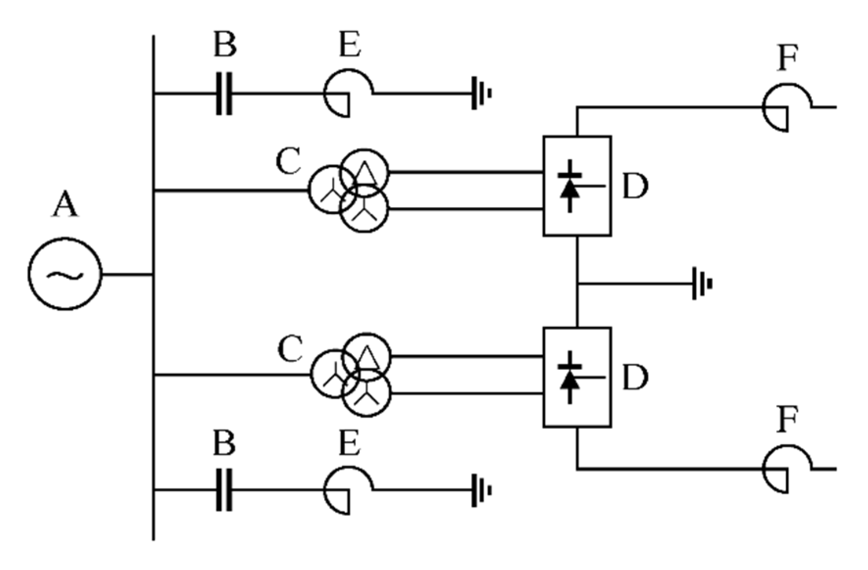
The valve control system is the core equipment of the direct current (DC) transmission system, and the task of it is to trigger and monitor the operation of the thyristor. The ABB converter valve control system is mainly composed of a thyristor control unit (TCU), valve control unit (VCU), thyristor monitoring unit (THM), and optical fiber transmission equipment. The TCU, which is fixed next to the thyristor, is a key component in the valve control equipment. It is responsible for the triggering and closing tasks of the thyristor. According to the actual situation, because there are numerous electromagnetic disturbance sources in the converter station, and the TCU is working at a high potential, TCU failure often occurs, resulting in abnormal work of the converter valve [5,6]. Although some TCUs used in converter stations now are installed in shields for electromagnetic field protection, it is subject to particularly large electromagnetic disturbances because of TCU working on the thyristor valve at a high potential. These electromagnetic disturbances will change irregularly, with multiple amplitude changes and a wide frequency range. The shielded cavity has a large number of resonance frequencies, which usually overlap with some electromagnetic disturbance frequencies, so it is difficult to make the TCU in the cavity reach a stable working state. In this case, the TCU is still likely to malfunction.

Once the TCU triggering the thyristor function fails and the voltage across the thyristor rises to about 6.8 kV, the TCU will issue a protective firing (PF) to turn on the thyristor in an emergency to prevent the thyristor from being damaged by high voltage. However, PF will cause a delay in valve conduction, and a direct current component will flow through the valve side winding of the converter transformer. Therefore, when the number of PF in the same converter valve reaches a certain number, in order to prevent the converter transformer from overstressing, the converter needs to be locked.

It is necessary to diagnose the TCU after the failure. At present, the research on circuit board fault diagnosis is relatively mature, including the Boolean difference method of the digital circuit [7], fault dictionary method of the analog circuit [8], parameter identification method [9], neural network method [10,11], and other methods. However, most of the traditional fault detection methods are offline detection, where the faulty component is found through measurement by a portable meter and then replaced. Although this type of method can guarantee a certain diagnostic accuracy, it greatly increases maintenance costs and also reduces the timeliness and efficiency of operation and maintenance. Therefore, there is an urgent need for a dependable online method of early warning to enable the system to perform real-time analysis of TCU-related data in an electromagnetic environment and fully excavate the abnormal data characteristics of the TCU. Based on it, the system could send an early warning before the TCU finally fails. Good failure warning can provide decision support for the operation and maintenance, inspection cycle, and maintenance plan of the converter valve, and it can greatly reduce the loss caused by the failure of valve control equipment, thereby ensuring the stability and reliability of the converter valve operation.

To solve the above problem, this paper analyzes the failure principle of the TCU in the electromagnetic environment based on the in-depth study of the valve control system of the ABB technical route and simulates the circuit board under the electromagnetic disturbance to see the distribution of its electric and magnetic fields. Then, in terms of the simulation results, a method of TCU failure early warning based on pattern matching and support vector regression (SVR) is proposed: according to the failure fault tree, the failure of the TCU is divided into several modes, and a failure mode library is constructed. SVR is utilized to generate failure predictor, where parameters are generated through grid search method (GS), genetic algorithm (GA), and particle swarm optimization (PSO). The best SVR parameters are selected through mean square error (MSE) and the square correlation coefficient r². For real-time exception logs, after pattern matching, the failure probability of each candidate mode is calculated to determine whether it exceeds the threshold. If the threshold is exceeded, the system will issue a danger warning. The example shows that the method can predict the failure condition of TCU in an electromagnetic environment well. Even if there are poor failure modes, and the new failure mode is unknown, the prediction accuracy of the system is still very high. In addition, the paper also compares the actual number of failures with and without warning. The results show that the failure avoidance rate is as high as 78.6%. This method can provide support for thyristor level maintenance.

2. Simulation Analysis of TCU in Electromagnetic Field

2.1. The Electromagnetic Environment Where the TCU Works

The TCU forms the thyristor valve level together with the thyristor element, damping circuit, voltage equalization circuit, and energy acquisition circuit. All the control and protection functions of the TCU are completed by electronic components, which are installed on a 7 cm × 19 cm circuit board without high-voltage components and high-power components. However, due to the installation location close to the thyristor, the TCU is often affected by great electromagnetic disturbance, which also restricts its normal operation.

The specific disturbance source distribution in the converter station is shown in Figure 1 [12,13].

In the actual working process of the converter valve, external electromagnetic disturbance acts on the TCU board and is coupled to the inside of the device through the device pins on the board. The device pins and other parts form a closed-loop, and the changing electromagnetic field acts on the device in the form of voltage or current to cause internal effects. When the electronic components are turned on or in a hot state, the internal carriers are already in an active state. Once there is a sudden electromagnetic field in the outside world, the charge area inside the device will suddenly gain a lot of energy, and the carrier movement will be more violent, which will cause some devices to fail or damage [14,15] and cause the failure of the TCU.

2.2. Simulation Analysis of TCU in Electromagnetic Field

The electromagnetic field generated by the electromagnetic interference source in the converter station can be divided into two parts according to nature: radiation field and induction field. The energy of the radiation field is separated from the radiator, while the energy of the induction field flows back and forth around the radiation source. In order to be easy to distinguish, usually according to the relationship between the field source wavelength λ and the distance r between the interference source and the sensitive device, the field is divided into the far-field (radiation field) and near-field (induction field).

Table 1. The difference between far-field and near-field.

Name	Another Name	Range	Electromagnetic Field Strength	Spatial Unevenness	Relationship Between Electric Field and Magnetic Field
Far-field	Radiation field	r >> λ	Slow	Small	Vertical, E = 377H
Near-field	Induction field	r << λ	Fast	Big	No clear relationship

shows the difference between the far-field and the near-field.

Import the TCU into the CST Microwave Studio, and set the material properties and boundary conditions. The CST simulation frequency is set to 0–2 GHz [16], and an electric field monitor and a magnetic field monitor are set up at 50 MHz.

For far-field disturbance, the plane wave can be utilized to simulate. Its propagation direction is set to (0,0,−1) and electric field direction to (1,0,0). The plane wave excitation is set to Gaussian pulse, as shown in Figure 2. The simulation model is shown in Figure 3.

The near-field disturbance source model is simulated by a pair of dipole wire antennas [17,18], which consist of two PEC cylinders (ideal metal conductors). The gap between the two cylinders is 2 mm. A port is added in the gap between the two PEC cylinders, where a Gaussian pulse signal with an amplitude of 1 V/m is applied, so that the antenna can radiate electromagnetic fields outward, as shown in Figure 4.

Theoretically, it is possible to place the wire antenna and the PCB in the same space for simulation, but this will divide the simulation space into tens of millions of grids, which greatly extends the simulation time. Therefore, for the purpose of appropriately reducing the time required for the simulation, the simulation ideas are now improved. As shown in Figure 5, the disturbance generated by the wire antenna itself is solved by simulation first, and then the simulation result as a near-field source is imported into the CST. At last, it is simulated with the PCB board, which not only improves the speed of simulation but also guarantees the rationality of simulation results.

After setting, run the simulation, and the result is shown in Figure 6.

From Figure 6, the electric and magnetic field distribution diagrams under far-field disturbance and near-field disturbance, it can be seen that the electric field intensity at the left and right ends of the board, some lines, and some chips is relatively large, and the magnetic field strength at the power supply line and part of the trigger line is relatively high. Based on the several places mentioned above, voltage probes are set at the voltage comparator U2, the double JK trigger U7, the monostable trigger U13, the transistor T44, the transistor D60, and power supply port (PSP), where the electric field strength is relatively large, to monitor the changes in the induced voltage. Current probes are set at the large power supply lines and trigger lines to monitor the changes in induced current. The eight probes mentioned above are numbers 1–8 in Figure 7, respectively.

We have considered setting up more voltage probes and current probes before but later found that even so, simulation results and prediction results have not been significantly improved. Besides, more resources are wasted if more probes are set up. Taken together, we have decided to select eight parts of the paper for monitoring. After the simulation, Figure 8 shows the time domain waveforms of eight probes.

Under the effect of electromagnetic disturbance, the components on the TCU appear oscillating-induced voltage and oscillating-induced current, but for different disturbances, there are differences in amplitude, changing trend, and attenuation speed. When the converter valve is operating normally, each component on the TCU has a working range. Once the time domain signal value of it exceeds this range under the electromagnetic field, the TCU may have the possibility of failure. Therefore, this paper takes the voltage and current information of key components on TCUs as the characteristic information of TCU condition monitoring, and the method based on pattern matching and regression analysis is utilized to analyze the characteristic information so as to realize the effective early warning of the TCU failure state.

3. Dynamic Pattern Matching Algorithm Based on Pattern Tree

3.1. Structural Failure Mode

By installing an expansion circuit board with voltage monitoring chips and current monitoring chips on the TCU, the voltage and current values of the key components of the TCU can be obtained in real-time. Based on these values, the working status of the TCU can be determined so that whether it will fail in an electromagnetic environment, it can be determined, too.

If the signal amplitude of a component exceeds the normal range at a certain moment, it can be considered that an exception has occurred. Subsequently, the number of new exceptions generated will be loaded into the error log. The exception information of the system at that moment can be attained from the historical error log. It is represented by a one-dimensional vector s_n.

$$s_n=[v_n^1,v_n^2,\dots ,v_n^j,\dots ,v_n^J]$$

(1)

where s_n corresponds to the n-th exception information, which represents the condition of the TCU at that time. v_n^j is the j-th variable in s_n, which is composed of the sum of the new error count g_k^j collected by the system before, so s_n can be written as the following formula:

$$s_n=[{\displaystyle \sum _{k=1}^n{g}_k^1},{\displaystyle \sum _{k=1}^n{g}_k^2},\dots ,{\displaystyle \sum _{k=1}^n{g}_k^j},\dots ,{\displaystyle \sum _{k=1}^n{g}_k^J}]$$

(2)

Each piece of exception information corresponds to the probability of TCU failure in this condition, where the value range is [0, 1]. 0 represents that the TCU is operating normally in this condition, and failure is unlikely to occur, while 1 represents that the TCU has been failed.

In reality, the source of electromagnetic disturbance is complex and varied, which leads to its non-unique failure. For example, some failures are caused by resistor aging, and some are caused by diode breakdown. Although it will eventually lead to the same failure result, the parameters exhibited are different because of different failure processes. Therefore, the failure mode is introduced in this paper. At this time, the failure probability is divided into several failure mode probabilities. The definition of failure mode probability is as follows:

$$h_n^m=\frac{e(n)}{e(N)}\times class(m)$$

(3)

where e(n) represents the total number of exceptions generated when the n-th exception information is recorded, e(N) represents the total number of exceptions finally generated when the TCU fails, m represents the failure mode, and class(m) is 1 or 0, respectively, indicating that the failure belongs to or does not belong to failure mode m. $h_n^m$ indicates the probability of failure of the TCU when the failure mode m is followed. The closer h is to 0, the more normal the condition of TCU; on the contrary, the more serious the condition. The closer $h_n^m$ is to 0, the more normal the condition of TCU; on the contrary, the more serious the condition.

3.2. Failure Mode Matching Algorithm Based on Mode Tree

When predicting TCU failure in an electromagnetic environment, it is necessary to judge its corresponding failure mode in real-time based on the characteristics of the exception information vector. The matching of the failure mode is a dynamic process.

The failure mode library {m₁,m₂,…,m_M} is extracted from all historical failure records. Extract the error variables whose cumulative error count is not 0 from the exception information matrix of each failure mode, and form {v₁ = x₁,v₂ = x₂,…,v_n = x_n} as the nodes of the tree, where x_i represents the cumulative exception count for vi when a new exception occurs. The first exception information vector corresponds to the root node and represents the system state where the error first occurs; the last exception information vector corresponds to the leaf node, which represents the system state that finally causes the TCU failure. Afterward, all failure modes are converted into their corresponding failure mode trees {tree₁,tree₂,…,tree_M}. Taking the first failure mode as an example, the corresponding failure mode tree tree₁ is as follows:

$$tre{e}_1=\{v_2=2\}\to \{v_2=4,v_1=1\}\to \{v_2=6,v_1=3,v_3=1\}$$

The variable with the first exception is v₂, and the cumulative count is 2. After the propagation of the intermediate error state, new exception variables v₁ and v₃ appear. The last set represents the state that causes the final failure of the TCU.

For a certain candidate pattern tree, the matching judgment is performed in sequence according to the order of depth traversal. First, starting from the root node, the matching degree calculation process is as follows:

Step 1: Calculate the number matching degree, value matching degree, and total matching degree of the same elements.

Based on the Jaccard similarity, the number matching degree between the real-time exception information vector A and the exception information vector B in a certain pattern tree is defined as follows:

$$sim(A_{num},B_{num})=\frac{count(A\cap B)}{count(A\cup B)}$$

(4)

where count(A∩B) represents the number of non-zero elements in the set after the intersection of the corresponding digits of A and B; count(A∪B) represents the number of non-zero elements in the set after the union of the corresponding digits of A and B.

Based on the Cosine similarity, the value matching degree between the real-time exception information vector A and the exception information vector B in a certain pattern tree is defined as follows:

$$sim(A_v,B_v)=\frac{{\displaystyle \sum _{i=1}^n{A}_{v_i}{B}_{v_i}}}{\sqrt{{\displaystyle \sum _{i=1}^n{A}_{v_i}^2}}\sqrt{{\displaystyle \sum _{i=1}^n{B}_{v_i}^2}}}$$

(5)

The total matching degree:

$$degree(s_n)=sim(A,B)=sim(A_{num},B_{num})\times sim(A_v,B_v)=\frac{count(A\cap B)}{count(A\cup B)}\times \frac{{\displaystyle \sum _{i=1}^n{A}_{v_i}{B}_{v_i}}}{\sqrt{{\displaystyle \sum _{i=1}^n{A}_{v_i}^2}}\sqrt{{\displaystyle \sum _{i=1}^n{B}_{v_i}^2}}}$$

(6)

when the matching degree is 0 < δ < sim(A,B) ≤ 1, it can be considered that the matching is successful, and then go to Step 2; if the matching degree requirement is not met, go to Step 3. The threshold δ can be adjusted according to the actual situation, and it is 70% by default.

Step 2: Record the matching degree (s_n) of the exception information vector, and calculate the total matching degree of the failure mode tree:

$$degree(tre{e}_i)={\displaystyle \prod _{j=1}^{n}degree(s_j)}$$

(7)

Then, the traversal pointer points to the next node of the pattern tree.

Step 3: Eliminate the failure mode from the candidate set, and update the candidate mode tree.

Step 4: Loop steps 1 to 3 to match the failure mode tree. In the matching process, by calculating the matching degree between the current failure process and multiple candidate mode trees, the failure modes that do not meet the requirements are dynamically eliminated. The matching degree of each remaining failure mode is sorted from high to low. According to the maximum value of the matching degree, it can be divided into known failure mode and unknown failure mode. If the maximum matching degree exceeds 70%, it is judged as a known failure mode; otherwise, it is an unknown failure mode. Then, import the exception information vector into the corresponding failure mode predictor to determine whether an early warning is needed.

4. Failure Predictor Based on SVR

4.1. Support Vector Regression Optimized by Particle Swarm Optimization

Support vector regression is based on the principle of support vector machines (SVM) and is widely utilized in the field of anomaly detection and prediction. Compared with general methods, SVR is suitable for solving the regression problem of high-dimensional features. It still has a good effect when the sample size is small or if the feature dimension is greater than the number of samples.

For the training sample set, S = {(x₁,y₁),(x₂,y₂),…,(x_n,y_n)}, where x_i ∈ Rⁿ is the input vector, and y_i ∈ R is the output value. The support vector machine regression function is shown in equation (8):

$$f(x)={\omega }^T\varphi (x)+b$$

(8)

where φ(x) is the kernel function of mapping data samples from low-dimensional space to high-dimensional space, ω is the vector of weight coefficients, and b is the offset.

Slack variables ξ_i and ${\widehat{\xi }}_i$ are introduced, and the equation (8) is transformed into an optimization problem of finding the objective function to minimize.

$$\underset{\omega ,b,{\xi }_i,{\widehat{\xi }}_i}{\min }\frac{1}{2}{\Vert \omega \Vert }^2+C{\displaystyle \sum _{i=1}^m({\xi }_i+{\widehat{\xi }}_i)}$$

(9)

The constraints are:

$$\{\begin{array}{l}f(x_i)-y_i\le \epsilon +{\xi }_i\\ y_i-f(x_i)\le \epsilon +{\widehat{\xi }}_i\\ {\xi }_i\ge 0,{\widehat{\xi }}_i\ge 0,i=1,2,\dots ,m\end{array}$$

(10)

where C is the penalty factor; ξ_i and ${\widehat{\xi }}_i$, respectively, represent the upper and lower limits of slack variables, and ε is the fitting accuracy of the function.

When solving the convex quadratic optimization problem, it can be transformed into its dual form. The Lagrangian function needs to be introduced in the calculation process. For nonlinear system regression problems, an appropriate kernel function K(x,y) = <φ(x), φ(y)> needs to be selected to map the data from the low-dimensional feature space to the high-dimensional feature space and perform linear regression in the high-dimensional feature space. The dual form of the optimization problem is shown in Equation (11):

$$\underset{\alpha ,\widehat{\alpha }}{\max }{\displaystyle \sum _{i=1}^m{y}_i({\widehat{\alpha }}_i-{\alpha }_i)-{\displaystyle \sum _{i=1}^m\epsilon ({\widehat{\alpha }}_i+{\alpha }_i)}}-\frac{1}{2}{\displaystyle \sum _{i=1}^m{\displaystyle \sum _{j=1}^m({\widehat{\alpha }}_i-{\alpha }_i)}}({\widehat{\alpha }}_j-{\alpha }_j)x_i^T{x}_j$$

(11)

The constraints are:

$$\{\begin{array}{l}{\displaystyle \sum _{i=1}^m({\widehat{\alpha }}_i-{\alpha }_i)}=0\\ 0\le {\alpha }_i,{\widehat{\alpha }}_i\le C\end{array}$$

(12)

Solve the solution of the optimization problem Formula (12) and calculate b. Consequently, the regression function can be attained:

$$f(x)={\displaystyle \sum _{i=1}^m({\widehat{\alpha }}_i-{\alpha }_i)K(x,x_i)+b}$$

(13)

Considering that the radial basis function (RBF) has a strong ability to calculate high-dimensional samples and has good generalization ability, the kernel function selected in this paper is RBF:

$$K(x,x_i)=\exp (-{\Vert x-x_i\Vert }^2/2{\sigma }^2)$$

(14)

In order to further improve the prediction performance of the SVR regression machine, an effective algorithm should be found to optimize the relevant parameters of the SVR. Since this paper utilizes the RBF kernel function for SVR nonlinear regression modeling, the RBF kernel parameter g and penalty parameter C are the two parameters that the SVR network needs to select. The prediction effect of g and C on the SVR regression network will have a great impact. Grid search method (GS) [19], genetic algorithm (GA) [20], and particle swarm optimization (PSO) [21] can be applied to optimize the parameters g and C of SVR, and they have varying degrees of applicability for different problems.

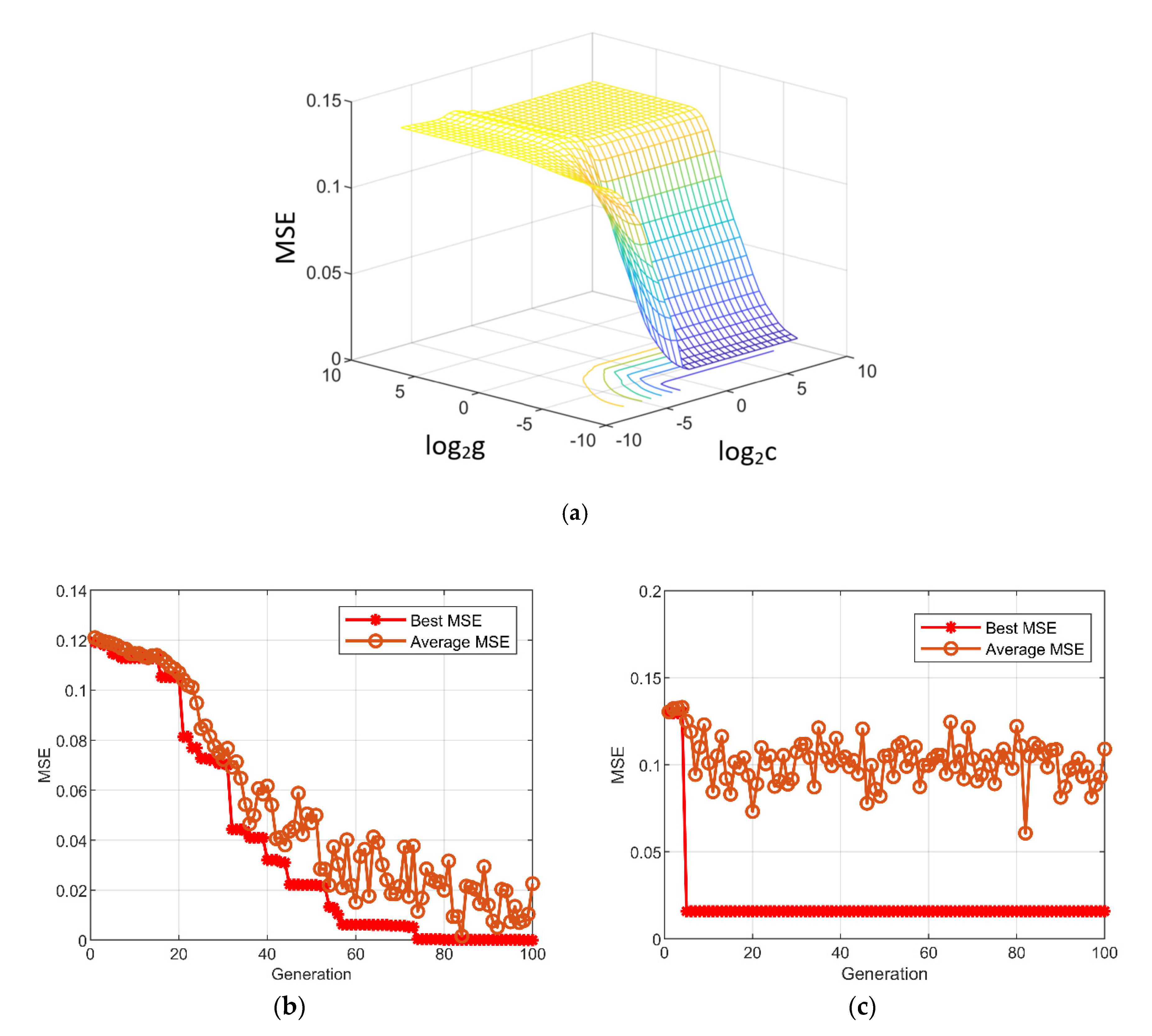
GS searches for all parameter combinations within a certain rectangular range according to a given step size and takes the Leave-One-Out method to cross-validate the sample set for all parameter combinations in the grid. Finally, MSE corresponding to each group (C, g) is drawn with contour lines, and the best (C, g) value is determined accordingly.

When GA is utilized for parameter optimization, binary coding is applied regularly. GA does not need to calculate all parameter points, while it can determine the global optimal solution through operations, such as selection, crossover, and mutation.

When using PSO for parameter optimization, the position and velocity of each particle are determined by the two-dimensional parameters (C, g). The PSO algorithm has a small amount of calculation and still shows excellent predictive ability in the case of a small training set.

This paper takes these three methods to obtain SVR parameters and then takes the method of K-fold cross-validation (K-CV) [22], which is one of the cross-validation methods, to compare the performance of the regression model and select the optimal C and g values.

4.2. Failure Predictor Based on SVR

Establish the relationship between historical exception information and failure modes, and construct a failure predictor based on regression analysis. In this way, according to the real-time exception information, it is possible to determine the failure stage it is in and determine whether it is necessary to issue an early warning.

Assuming that the TCU is in operation, error logs {p₁,p₂,…,p_n} are generated at the time {t₁,t₂,…,t_n}. These logs are recorded in the database and contain all the information of each exception. Then, the regression analysis is performed, which is mainly divided into the following three steps:

Step 1: Extract information from each error log p_n, construct an exception information vector s_n, and evaluate its failure mode probability;

Step 2: Form a (J + 1) × N—order matrix X and failure mode probability column vector Y_m. Among them, J is the number of variables in each exception information vector, and N is the number of exception information vectors;

$$X=\left(\begin{array}{l}\begin{array}{ccc}1& v_1^1& v_1^2\\ 1& v_2^1& v_2^2\\ ⋮& ⋮& ⋮\end{array}\begin{array}{ccc}\dots v_1^j& \dots & v_2^J\\ \dots v_2^j& \dots & v_2^J\\ \ddots ⋮& \ddots & ⋮\end{array}\\ \begin{array}{ccc}1& v_n^1& v_n^2\\ ⋮& ⋮& ⋮\\ 1& v_N^1& v_N^2\end{array}\begin{array}{ccc}\dots v_n^j& \dots & v_n^J\\ \ddots ⋮& \ddots & ⋮\\ \dots v_N^j& \dots & v_N^J\end{array}\end{array}\right)$$

(15)

$$Y_m={\left[h_1^m{h}_2^m\cdots h_n^m\cdots h_N^m\right]}^T$$

(16)

Step 3: Utilize SVR to construct a failure mode probability predictor for failure mode m. For any real-time exception information vector s_n, the predictor based on SVR can be applied to predict the occurrence probability of failure mode m, that is, the estimated value of failure mode probability ${\widehat{h}}_n^m$.

The closer the failure probability is to 0, the more normal the condition of TCU, so it is essential to ensure that ${\widehat{h}}_n^m$ is less than the threshold α ∈ [0, 1]; otherwise, the TCU is in a dangerous situation, and the entire system may malfunction. In addition to this, time issues also need to be considered because it takes time for system response and personnel to perform maintenance. Once the total time exceeds the time remaining for the TCU to fail, then this warning is considered invalid because it has not succeeded in avoiding the failure and wasted system resources. Therefore, it is also necessary to comprehensively consider the impact of the early warning time.

Figure 9 shows the flow chart of the early warning method. Suppose the time from the recording of the n-th exception information to the failure of the TCU is t_r, the time when the predictor issues an early warning and the system responds is t_p, and the maintenance time is t_q If t_p + t_q ≤ t_r is satisfied, it means that the warning issued at this time is valid, and then the system can promptly respond and perform maintenance, which can ultimately avoid failure. If t_p + t_q > t_r, even if the alarm is issued at this time, the system could not handle it in time, which requires manual maintenance, and the warning is invalid. When an invalid early warning is issued, it is essential to slightly lower the failure mode probability threshold so as to ensure that all work can be completed in enough time.

4.3. Failure Prediction and Alarm

Based on the failure mode probability and early warning time obtained by regression analysis, specific failure modes can be predicted and alarmed.

For the known failure mode m, effective early warning can be carried out if the formula (17) is satisfied:

$$\{\begin{array}{l}{h}_n^m\ge {\alpha }^m\\ \frac{t_p^m+t_q^m}{t_r^m}\le 1\end{array}$$

(17)

In the beginning, all $h_n^m$ are set to default value 0.6, and an effective warning will be issued when the probability is higher than 0.6, and the warning time satisfies the requirements. Then, the values of each $h_n^m$ are constantly adjusted when an invalid warning appears.

When an unknown failure mode appears, the model proposed above is not applicable because of no corresponding exception information. At this moment, the traditional probability statistics method is utilized to judge it.

$$h_n=\frac{failure(s_n)}{failure(s_n)+success(s_n)}$$

(18)

where failure(s_n) represents the number of unissued warnings of s_n in all known modes, and success(s_n) represents the number of warnings of s_n in all known modes. h_n represents the unknown failure mode. By judging whether h_n exceeds the threshold β ∈ [0, 1], it can be judged whether the system has failed. If the requirements are met, the system will also issue a failure warning. After this kind of unknown failure mode occurs, the exception information vector, failure mode probability, and various time parameters will be recorded to the database to expand and improve it. Subsequently, if this type of failure occurs next time, it can be treated as a known failure mode.

Finally, the accuracy P is applied to describe the accuracy of failure warning. Assuming that the system predicts that the TCU will fail in the future, it is considered positive at this time. This warning may be correct (true positive, TP) or wrong (false positive, FP). The calculation formula of the failure warning accuracy is:

$$P=\frac{TP}{TP+FP}$$

(19)

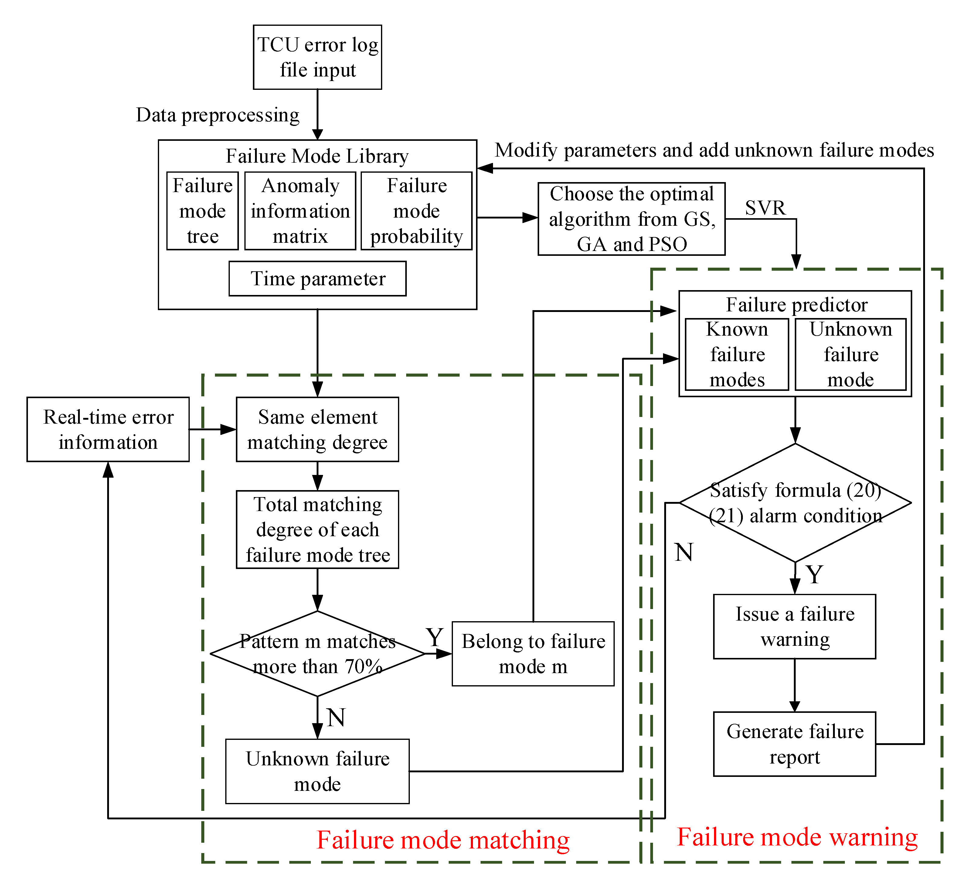
In summary, the process of the TCU failure early warning method in an electromagnetic environment based on pattern matching and SVR is shown in Figure 10.

5. Experiment and Analysis

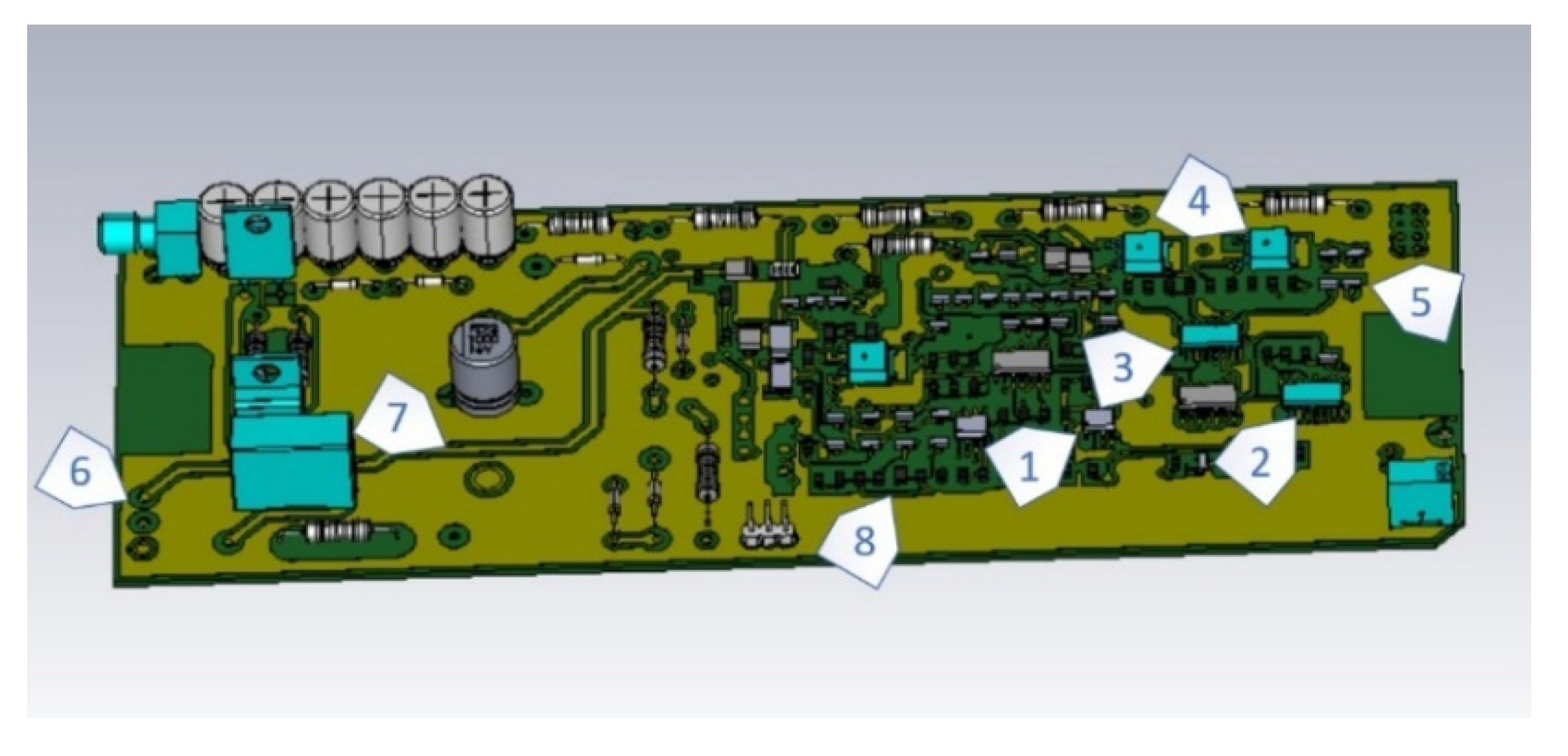
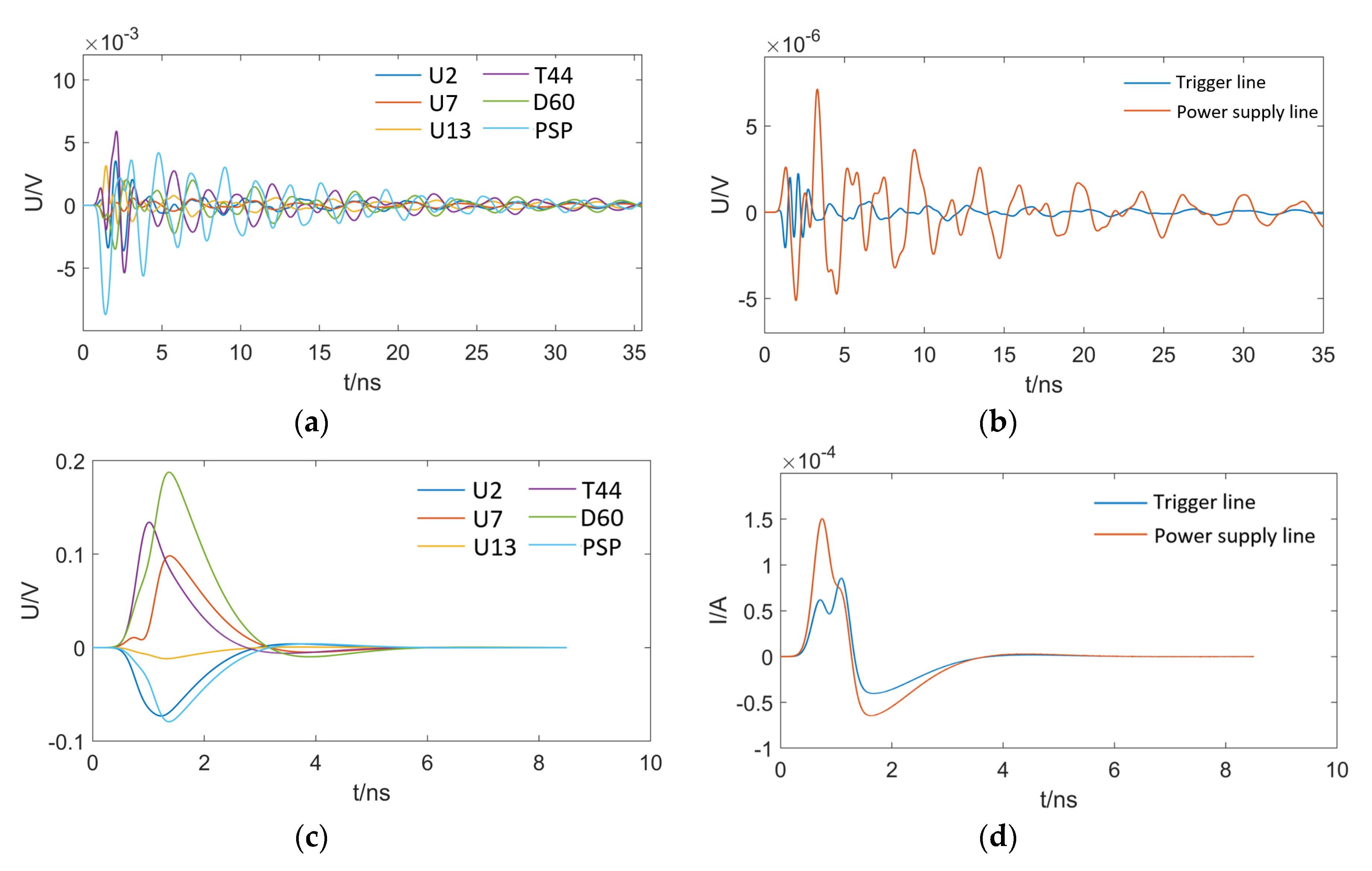
Take the ABB technical route valve control system used in a converter station in Jiangsu Province as an example, select the chips U2, U7, U13, transistors T44, D60, and the power supply port on the TCU circuit board to monitor their voltage, select the power supply line and trigger line to monitor their current, a total of eight variables. Then, run the monitor to capture the error log of TCUs during the running time and divide it into two parts. The first part covers most of the early data, which accounts for about 80% of the total data. It is applied to construct a preliminary prediction model. The second part accounts for about 20% of the total data. It is utilized to test the advantages and disadvantages of the model and make the model as best as possible. After reaching the expected goal, put it into the actual running system to make predictions.

The system first extracts nine failure modes from historical failure information and then generates failure mode trees to construct failure predictors. Taking failure mode 3 as an example, as shown in

Table 2. New error count for each variable in the error log.

k	…	${\mathit{g}}_{\mathit{k}}^3$	${\mathit{g}}_{\mathit{k}}^4$	${\mathit{g}}_{\mathit{k}}^5$	${\mathit{g}}_{\mathit{k}}^6$	…
1	…	0	1	0	0	…
2	…	0	2	0	1	…
3	…	0	2	1	0	…
4	…	0	0	1	0	…
5	…	0	1	0	2	…
6	…	0	3	1	0	…
7	…	1	1	2	1	…
8	…	0	0	0	2	…
9	…	0	3	1	2	…
10	…	0	3	3	1	…
11	…	0	3	3	4	…
12	…	0	4	4	2	…

and

Table 3. Exception information matrix and failure mode probability.

n	…	${\mathit{v}}_{\mathit{n}}^3$	${\mathit{v}}_{\mathit{n}}^4$	${\mathit{v}}_{\mathit{n}}^5$	${\mathit{v}}_{\mathit{n}}^6$	…	${\mathit{h}}_{\mathit{n}}^3$
1	…	0	1	0	0	…	0.018
2	…	0	3	0	1	…	0.073
3	…	0	5	1	1	…	0.127
4	…	0	5	2	1	…	0.145
5	…	0	6	2	3	…	0.2
6	…	0	9	3	3	…	0.273
7	…	1	10	5	4	…	0.364
8	…	1	10	5	6	…	0.4
9	…	1	13	6	8	…	0.509
10	…	1	16	9	9	…	0.636
11	…	1	19	12	13	…	0.818
12	…	1	23	16	15	…	1

, the abnormal value of this failure mode is reflected in one chip, two transistors, and the power supply port, corresponding to the variables $v_n^3$, $v_n^4$, $v_n^5$ and $v_n^6$ in s_n.

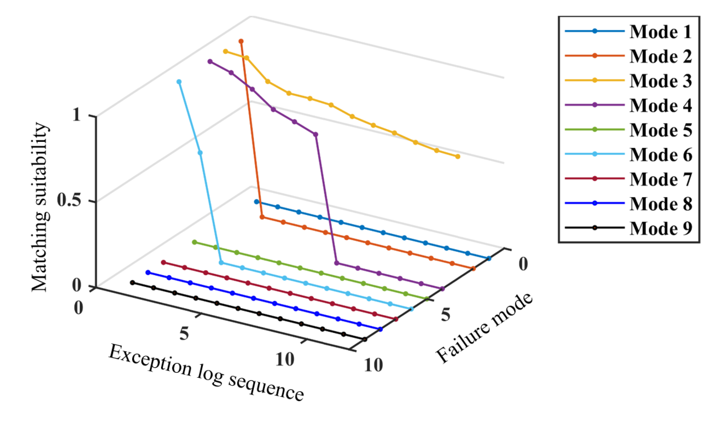
When the real-time exception information vector is continuously imported into the failure predictor, the system first dynamically matches the failure mode according to the failure mode matching algorithm in part 3.2. Figure 11 shows the matching process of the exception information vector in a certain period of time.

As can be seen from Figure 11, after the first exception information vector is generated, modes 2, 3, 4, and 6 are very similar to it, so these four modes are listed as candidate failure modes. Then, as the subsequent exception information vector is continuously generated, the conditions for pattern matching become more and more complicated, and there are fewer and fewer candidate failure modes. Mode 2, mode 6, and mode 4 are eliminated in turn, and the only mode 3 is left in line with the current TCU failure mode.

SVR is applied to construct the failure predictor of each mode, and GS, GA, and PSO are used to obtain the parameters for each mode. The three algorithms all adopt the K-CV cross-validation method and are completed under the MATLAB software platform [23,24].

Taking the above-mentioned mode 3 as an example, the optimization processes of GA, GS, and PSO are shown in Figure 12a–c, respectively. The ordinate in the figure represents MSE.

Through the optimization of different algorithms, different values of the penalty parameter C and the kernel parameter g can be obtained. Different C or g corresponds to different generalization capabilities and application effects of the model. This paper chooses MSE and squared correlation coefficient r² to measure. The calculation formulas of MSE and r² are as shown in Formula (20) and Formula (21), and the optimization results of the three methods and the values of MSE and r² are shown in

Table 4. Comparison of SVR indicators under different algorithms. GS-SVR, support vector regression optimized by grid search method; GA-SVR, support vector regression optimized by genetic algorithm; PSO-SVR, Support vector regression optimized by particle swarm optimization.

Parameter Optimization Algorithm	Parameter C	Parameter g	MSE	r2
GS-SVR	0.5	0.0039	0.00375	0.98291
GA-SVR	93.0084	0.0001	0.00565	0.99350
PSO-SVR	0.44011	0.01	0.00335	0.99679

.

$$\mathrm{MSE}=\frac{1}{m}{\displaystyle \sum _{i=1}^m{(f(x_i)-y_i)}^2}$$

(20)

$$r^2=\frac{{(m{\displaystyle \sum _{i=1}^{m}f(x_i)y_i-{\displaystyle \sum _{i=1}^{m}f(x_i)}{\displaystyle \sum _{i=1}^m{y}_i}})}^2}{[m{\displaystyle \sum _{i=1}^{m}f{(x_i)}^2}-{({\displaystyle \sum _{i=1}^{m}f(x_i)})}^2][m{\displaystyle \sum _{i=1}^m{y}_i{}^2}-{({\displaystyle \sum _{i=1}^m{y}_i})}^2]}$$

(21)

In general, changing the penalty coefficient C can adjust the complexity of the model and the empirical risk. If C is too small, sometimes the training error will be too large; if C is too large, although the training accuracy is improved, the generalization ability of the regression model decreases. That is, the MSE of the training set is very low, and the MSE of the test set is very high. The appropriate penalty coefficient can avoid the influence of abnormal data in the sample, thereby improving the stability of the model. In Table 4, the parameter C obtained by GA is too large, reaching 93.0084, while parameter C of GS and PSO is moderate.

The kernel parameter g reflects the degree of correlation between the support vectors. If g is too small, the connection between the support vectors will be slack, the model will become complicated, and the generalization ability will decrease; if g is too large, the connection between the support vectors will be too close, and the accuracy will be difficult to meet the requirements. In Table 4, the magnitude of g obtained by GA and GS is very small, which is 10⁻³, less than 10⁻² of PSO.

Regarding the mean square error MSE and the square correlation coefficient r², the more MSE tends to 0, the higher the regression accuracy; the closer r² is to 1, the better the algorithm stability. The MSE and r² of the three methods in the table are all ideal, and there is not much difference, which means that the regression effect is good.

In fact, it will not be so complicated in actual engineering applications. Parameter selection is required when a certain failure mode appears for the first time. Neither the parameter c nor the parameter g can be too large or too small because this will affect the effect of the SVR. For our system, c generally takes 0.1–10, and g generally takes 0.001–0.05. Therefore, when MSE is less than 0.01, and r² is greater than 0.95, the c and g obtained by the optimization algorithm only need to be in the above-mentioned range (all three methods in the paper are satisfied). After that, the two coefficients will be stored in the system and applied when the next failure of the same type occurs.

The MSE and r² of PSO are a little more ideal than others by comparison. Therefore, this example adopts the method of SVR optimized by PSO (PSO-SVR) to predict the failure of TCU in an electromagnetic environment.

Import 851 groups of historical exception information matrix, and set the threshold of the matching degree of each pattern to 70%. The accuracy of pattern matching can be evaluated by the confusion matrix [25]. The numbers on the diagonal of the matrix are the correct numbers, as shown in Figure 13.

It can be calculated from the confusion matrix in Figure 13 that the accuracy of pattern matching is as high as 91.07%, and the error ratio is 8.93%. After completing the pattern matching, calculate the failure mode probability corresponding to the real-time exception information vector so as to perform failure prediction.

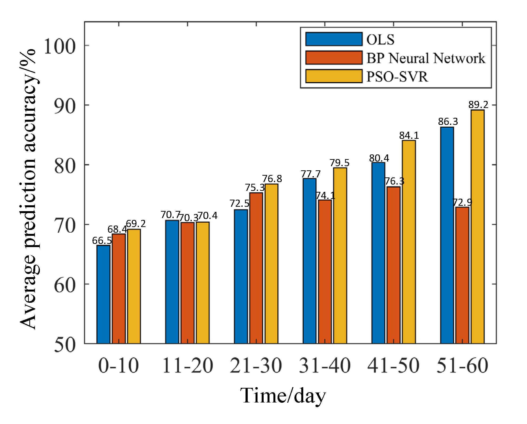
Figure 14 shows the comparison of prediction accuracy after running the model on the target system for 60 days. Yellow corresponds to the method proposed in this paper, blue represents the ordinary least squares (OLS) method [26], and red corresponds to the traditional neural network method [27]. As can be seen from Figure 14, as time goes by, the average prediction accuracy of this method is also steadily increasing. In the beginning, the three methods take the same data; therefore, the average prediction accuracy of them is very close. However, as time and the electromagnetic environment changes, new failure modes of TCU occur, which are difficult to identify with traditional neural network methods. Different from the traditional method, the method proposed in this paper and the OLS method can add unknown failure modes to the failure mode library for use in the next similar failure. Therefore, the prediction accuracy gradually increases in the middle and late stages. Compared with the general OLS, PSO-SVR in this paper has the advantage of always having the global optimal value in the training process. Additionally, the generalization ability of PSO-SVR is strong, the solution space is sparse, and the convergence speed is fast. The calculation example also proves that the method in this paper is slightly better than the traditional OLS regression method.

As shown in

Table 5. A comparison of real failure counts with and without warning.

Time/Week	1	2	3	4	5	6	7	8
Predicted failure count/time	24	29	34	26	25-	31	36	32
Real failure count without warning/time	26	34	27	25	-	-	-	-
Real failure count with warning/time	-	-	-	-	5	8	5	6

, the TCU is tested in weeks 1–8. The TCU early warning system is not operated in weeks 1–4, and it is operated in weeks 5–8. The electromagnetic environment, temperature, humidity, and other external conditions of the four weeks before and after should be the same as possible. Note that the failure mode library at this time has been constructed and corrected. In weeks 1–4, the predicted failure counts are basically equivalent to the actual failure counts that occur without warning, indicating high prediction accuracy. When the true value is higher than the predicted value, it indicates that the predictor has underreported. When the predicted value is higher than the true value, it indicates that there is a certain overstatement. There will be more or less misreports, but the overall prediction accuracy is about 90%. In weeks 4–8, with the participation of the early warning system, the average failure rate decreases from 28 times per week to 6 times per week. The failure avoidance rate is 78.6%, which indicates that the early warning effect is obvious.

6. Conclusions

Based on simulation analysis and real-time monitoring of the abnormal data of sensitive components on the TCU, this paper proposes a TCU failure early warning method based on pattern matching and SVR in the electromagnetic field, which combines pattern matching and regression analysis. Taking into account the failure type and warning time, effective failure warning is realized through continuous expansion of the failure mode library and correction threshold. The main contributions of the paper are as follows:

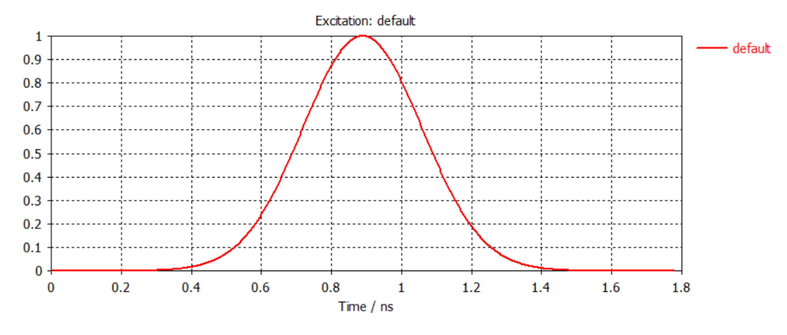
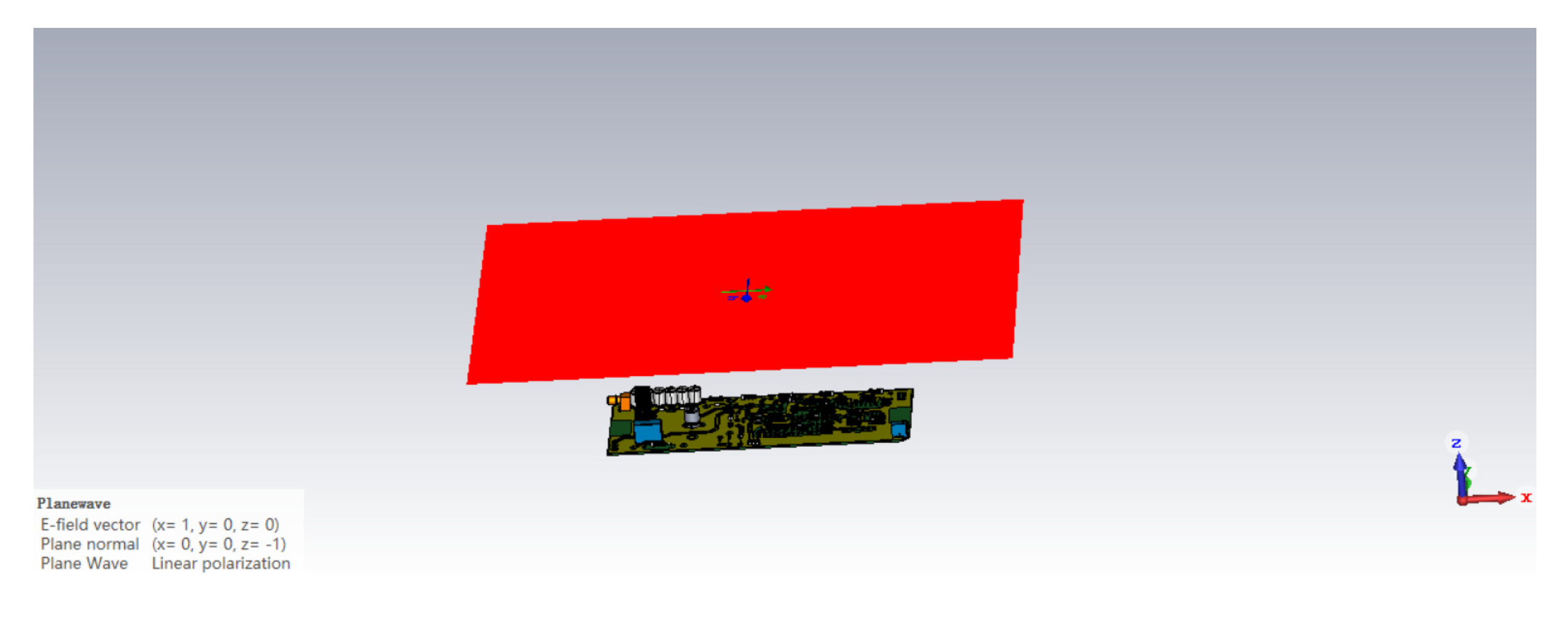
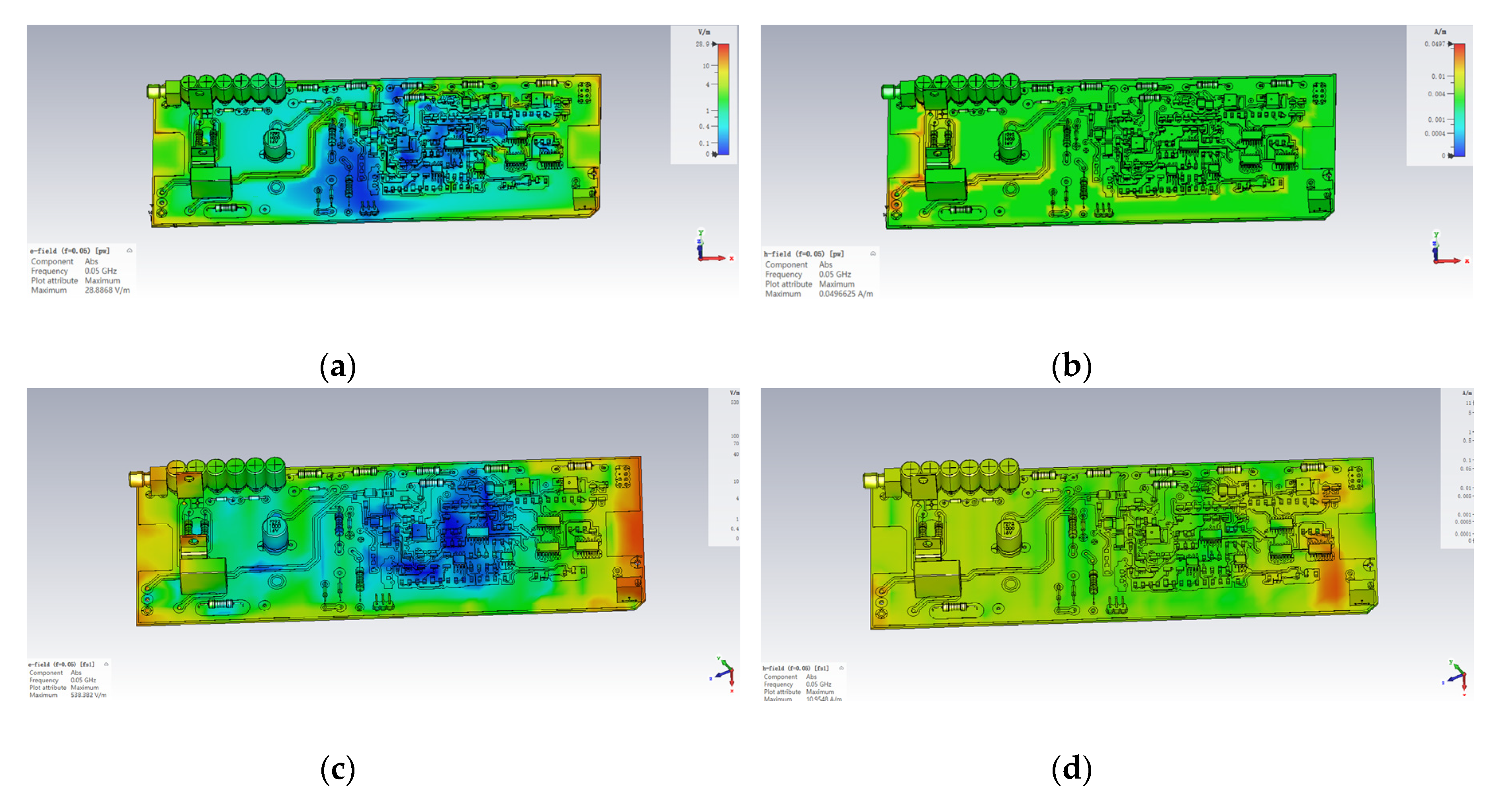
(1) The electromagnetic disturbance process of the TCU is simulated and analyzed. The electric and magnetic field distributions on the TCU under different disturbance sources are obtained, and important sensitive components are selected to monitor the voltage and current information in real-time;

(2) Establish a set of TCU failure warning methods based on dynamic mode matching and SVR. The optimization effects of GA, GRID, and PSO are compared, and the best PSO for parameter optimization is selected, which can achieve a TCU failure prediction accuracy rate of over 89%. Besides, the failure avoidance ratio reaches 78.6%.

The results verify that the proposed method can match the TCU failure mode in the electromagnetic environment well and issue an early warning, which has practical engineering application value.