1. Introduction
Recently, global interest in and demand for microgrids has been increasing, particularly with regard to the convergence of power systems. Information and communication technology (ICT) is emerging as the core technology of microgrids. The microgrid is accelerating the growth of the energy industry by taking the lead in responding to the new climate regime, and it is being used for a variety of purposes, such as economic power supply, leading to reduced demand-side electricity rates. The global microgrid market is expected to reach USD 67.6 billion by 2021, and the annual average growth rate from 2018 to 2021 is expected to be 21.7% [
1]. As one of the components of the microgrid, an energy storage system (ESS) can contribute to enhancing the quality of power and securing the stability of the power grid by balancing the output and supply and demand of unstable distributed resources.
One of the most salient issues in the microgrid environment, where energy supply and demand has been rapidly increasing in recent years, is minimizing energy costs by reducing energy consumption, maintaining the energy supply and demand balance, and increasing renewable energy sources (RES) utilization. To this end, the development of an energy management system (EMS) is essential. An EMS reinforces operational functions, such as adjusting the amount and schedule of charging and discharging through the efficient control of the ESS and power conditioning system (PCS), and manages the overall power flow. In addition to simple monitoring, it is linked with sensors and measurement equipment to analyze consumer consumption patterns and manage information on all power activities so it can be operated with optimum efficiency.
This study proposes an operation scheduling model to be applied to the digital twin in order to solve the difficulty of grasping the physical meaning in the complex situation of the system and achieve the synchronization technology between virtual and real spaces. By implementing the actual microgrid in virtual space, the composition of the microgrid can be changed in various ways, and the system operation can be improved by applying more data and algorithms. The proposed operation scheduling model was designed by applying the daily ESS optimal charging/discharging schedule to the machine learning technique to minimize electricity bills. If there is a change in the system, such as the addition or removal of microgrid components, changing the operation mode and modifying the objective function and constraints is inevitable, and it is difficult to immediately apply this to the actual system. A digital twin that works in a way similar to real systems in virtual space can solve these problems.
Data collected through an EMS were used, and the characteristics of the actual ESS embedded in the data were derived and reflected in the model. Various methods have been studied to establish an ESS charging/discharging schedule [
2,
3,
4,
5], and most of them have been defined as optimization problems. The ESS schedule was established by applying techniques such as linear programming (LP), particle swarm optimization (PSO), and simulated annealing (SA) [
6,
7,
8]. There is currently a scarcity of studies that have applied artificial intelligence to establish an ESS optimal scheduling by extracting the features of the data that can be applied to the microgrid operation scheduling. The existing methods have a high understanding of the ESS and must be implemented to satisfy the control variables and constraints, but it is difficult to accurately optimize the complex ESS structure due to the nonlinearity and uncertainty of the system information. If existing theories and calculation methods are complex, problems can be solved effectively by establishing a data-based model and applying machine learning. A model was implemented to reduce errors through numerous iterative learnings based on past data and to predict future behavior with new input data. Using these data, machine learning techniques were applied to the ESS scheduling, and the similarity with the optimization-based ESS scheduling in actual operation was verified through a case study. This has the advantage of implementing a model that sufficiently reflects the characteristics of the system by grasping the physical meaning only with the data, without knowing the information pertaining to the equipment. By modeling the virtual space, we were able to resolve the difficulty of establishing an optimal scheduling of the ESS and improve the stable operation and efficiency of the microgrid.
2. Background
In this section, we briefly summarized the background on the optimal scheduling of the microgrid for the digital twin into two categories: digital twin and machine learning.
2.1. Digital Twin
The concept of the digital twin [
9,
10] was first introduced by Grieves in 2002, and NASA formalized its definition in 2012. Digital twin technology utilizes IoT (Internet of Things), clouding computer and cyber physics systems developed to detect physical problems more quickly and to better predict physical outcomes.
Figure 1 illustrates the digital twin concept for microgrid.
The definition of digital twins as defined in [
9] are as follows:
Digital twin: The digital twin is a set of virtual information constructs that fully describe a potential or actual physical manufactured product from the micro atomic level to the macro geometrical level.
Digital twin prototype: This type of digital twin describes the prototypical physical artifact. It contains the informational sets necessary to describe and produce a physical version that duplicates or twins the virtual version.
Digital twin instance: This type of digital twin describes a specific corresponding physical product that an individual digital twin remains linked to throughout the life of that physical product.
Digital twin environment: This is an integrated, multidomain physics application space for operating on digital twins for a variety of purposes.
It detects system failure in advance and monitors its health in real time to help predict failure. In particular, it is difficult to grasp the physical meaning in a complex situation of the system, so it is not easy to quickly grasp the failure until the system actually fails. The advantages of the digital twin are as follows [
11,
12,
13,
14,
15]:
2.2. Machine Learning
Machine learning [
16,
17] is a technique that learns empirical characteristics and makes predictions or decisions using past data. In 1959, Arthur Samuel defined it as an area of research aimed at giving computers the ability to learn, without explicitly writing programs [
18]. Since then, technology that combines machine learning and big data, which has recently been of interest, has been actively researched.
Machine learning identifies patterns, rules, and meanings fundamental in data through learning and improves performance by itself through repeated learning and trial and error. As shown in
Figure 2, machine learning types [
19,
20,
21,
22,
23] are divided into supervised learning, unsupervised learning, and reinforcement learning. Supervised learning uses a set of labeled learning data and iteratively learns to reduce the error between the predicted value and the actual correct answer through the features of the data. In supervised learning, there are regression and classification, data mainly are predicted by regression, and the training data are learned to determine a group of input data by classification. Unsupervised learning without labels in a dataset learning based on the features of data is mainly used to solve problems such as clustering. Clustering such as
k-means, Gaussian mixture, and hierarchical groups similar data together to identify data patterns. Reinforcement learning is a technique that maximizes the reward that the agent gets through interaction with the environment, and learns an algorithm that determines the next action by receiving feedback on each action.
2.3. NARX
Nonlinear autoregressive with external input (NARX) [
24] is a nonlinear autoregressive neural network with external inputs. It learns to predict the original time series using the previous value of one time series, a feedback input value, and a second time series, which is an external time series [
2]. It is a two-layer feedforward network that has a sigmoid transfer function in the hidden layer and a linear transfer function in the output layer. As shown in
Figure 3, the output
y(
t) can be trained efficiently through an open feedback loop that is fed back to the network input through delay.
NARX with exogenous input is a cyclic dynamic network, and the feedback connection includes several layers, which are shown in Equation (1).
Here, the next value of the dependent output signal y(t) is regressed from the previous values of the output signal and the previous values of the independent (exogenous) input signal. The NARX model can be implemented using a feedforward neural network that approximates the function f. The input value to the feedforward network is more accurate, and so the resulting network has a pure feedforward architecture and can be used for more efficient algorithm training. The output y(t) can be trained efficiently through an open feedback loop that is fed back to the network input through a delay. The true output value can be used during the network training, and therefore, the actual output can be used instead of feeding back the expected output with the above open-loop architecture. NARX is advantageous because the input value to the feedforward network is more accurate, and because the resulting network has a pure feedforward architecture, a more efficient algorithm can be used for training.
The training was performed using the Levenberg–Marquardt algorithm. This algorithm combines the Gauss–Newton method and the gradient descent method. When it is far from the solution, it operates in the gradient descent method, and when it is near the solution, the Gauss–Newton method is used to find the solution. This method is mainly used for nonlinear least-squares problems because it can obtain the solution in a more stable manner than the Gauss–Newton method. It is more likely to find the solution, even when the initial value is far from the solution, and does so relatively quickly. The equations are shown in (2) and (3).
The Levenberg–Marquardt algorithm improves the Gauss–Newton method by reducing the risk of divergence and finds the solution more stably. When p is updated with the current μ value, μ continues to increase until E(p) decreases if E(p) increases, and μ being decreased to the original default value means minimum value if E(p) decreases.
2.4. Decision Tree
Decision trees (DT) are mainly used in data mining and are effective when predicting results or classifying data using a regression tree or a classification tree, according to the purpose. There is little need to process the data, and even with a large data set, the computation time is shorter than that for other algorithms. However, there is a risk of overfitting and creating a complex tree. The building strategy for Regression Tree is summarized in Algorithm 1 [
25].
| Algorithm 1. Building a Regression Tree [25] |
Use recursive binary splitting to grow a large tree on the training data, stopping only when each terminal node has fewer than some minimum number of observations. Apply cost complexity pruning to the large tree in order to obtain a sequence of best subtrees, as a function of Use k-fold cross-validation to choose . That is, divide the training observations into k folds. For each k = 1,…,K:
- (a)
Repeat Steps 1 and 2 on all but the kth fold of the training data. - (b)
Evaluate the mean squared prediction error on the data in the left-out kth fold, as a function of α.
Return the subtree from Step 2 that corresponds to the chosen value of α.
|
2.5. MARS
As one of the nonparametric regression methods, multivariate adaptive regression splines (MARS) is a nonlinear modeling method for the relationship between independent and dependent variables. MARS is a regression model that models data more effectively, and automatically determines the parameters based on data. It is suitable for analyzing a large set of data because it can perform various and complex large-scale dynamic calculations [
26].
Bi(
x) represents the basis function for each section, and
Ci represents the coefficient value for the corresponding basis function. When the variable section is divided into two sections based on
t, it appears in the form of a hinge function. Here,
t is the inflection point, which is the point at which the influence of the variable is reinforced or converted.
During the pruning process, MARS considers the possibility of overfitting. Its goal is to find a subset of the basis function with the minimum generalized cross-validation (
GCV) value.
The purpose of the MARS procedure is to combine recursive partitioning and spline fitting to best preserve the positive aspects of both, while being less vulnerable to adverse properties. In the regression analysis, it is a technique that quickly finds the spline basis function useful for fitting by using the subset selection method. Its advantage is that it is suitable for analyzing a large set of data because the form of the result is easy to interpret and the algorithm is simple.
3. Optimal Scheduling of ESS
This section describes data collection, configuration, and experimentation for learning and trialing the optimal ESS charging/discharging scheduling technique.
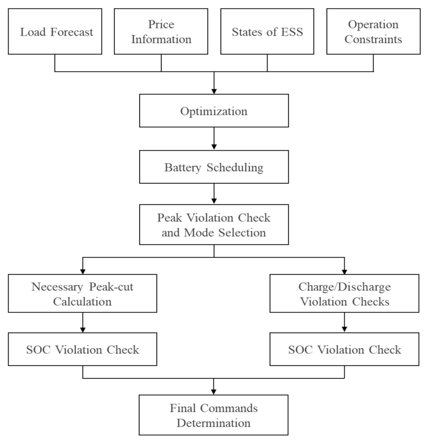
Figure 4 shows the optimal scheduling process for ESS. The proposed algorithm does not apply an optimization technique to establish an ESS charging/discharging schedule, and so it is implemented as a black box using machine learning without setting the objective function and constraints separately.
3.1. Original Scheduling
The ESS daily optimal scheduling [
27] such as
Figure 4 applied to the EMS uses an optimization-based algorithm, and an objective function is defined to maximize the savings in electricity bills. The rated charging/discharging output of the ESS, the battery capacity of the ESS, and the minimum and maximum power reception of consumers were set as constraints.
3.2. Simulation Data
The actual ESS operation data collected from November 2019 to July 2020 from the EMS of the actual microgrid and the time-of-use (TOU) tariff information [
28] by time were used. The data measured hourly were collected and classified into working days, Saturdays, and holidays. Only working days were used. The rates and time zones are different for each season, and therefore, February, May, and July were set as test months representing winter, spring, summer, and autumn. A total of 144 samples were tested on 6 days per season. Date, time, TOU tariff, State of Charge(SOC), and power of ESS information were selected as input data, and because the size of the data differed, all collected operation data were normalized and used (0, 1). From the collected operation data, 720 samples of the training data, 144 samples of the verification data, and 144 samples of the experimental data were set.
Figure 5 provides information regarding the case study subject, which consisted of an ESS with a battery capacity of 500 kWh and a PCS capacity of 250 kW.
Figure 6 illustrates the amount of charging and discharging actually operated by the ESS.
3.3. TOU Tariff
South Korea follows the Korea Electric Power Corporation(KEPCO) electricity tariff system [
28] and applies the rates in six categories according to the purpose of the electricity use (contract type: residential, general, industrial, educational, agricultural, and streetlight). The differential rate system for each season and time zone is a system whereby high rates are applied during peak load times in winter and summer when power consumption increases, and low rates are applied to light and intermediate loads in spring and autumn when electricity consumption is relatively low. It contributes to the stabilization of power supply and demand by strengthening demand management, and reflects the difference in the supply cost by season and time zone, which occurs according to the size of the power demand. The seasons were divided into spring from March to May, summer from June to August, autumn from September to October, and winter from November to February. Time zones were divided into light load, intermediate load, and maximum load. The time zones applied by season are shown in
Table 1.
The industrial rate system is divided into types A and B according to the contract demand in
Table 2, and the electricity rate was calculated using the high-voltage type A option 2 rate system for industrial power as of 2020. Industrial type B is applied when the user contract demand is 300 kW or more.
3.4. ESS Scheduling
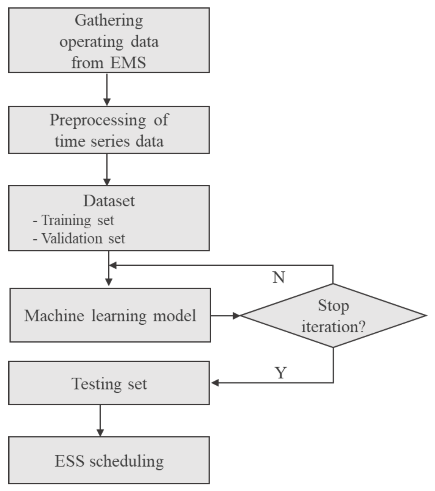
The ESS has different objective functions for each usage, and accordingly, constraints must be set differently. The characteristics of ESS and PCS should be fully understood and reflected in the objective function and constraints in order to derive a result suitable for the purpose. These processes can be shortened using machine learning, and optimal charging and discharging schedules can be established by learning, for example, the charging/discharging pattern of ESS using only past ESS operation data, without reflecting the physical information of the facility, such as capacity of ESS and PCS, and charging and discharging efficiency. Among the techniques commonly used in data-driven models, the daily ESS hourly schedule was established using the decision tree and NARX, which are supervised learning methods, and MARS, which is a nonlinear regression model. Based on past operation data, the algorithm was modeled to plan the charging/discharging of the ESS without defining, for example, any objective function or constraints. The experimental process is shown in
Figure 7. In order to prevent overfitting the models, a simulation was performed using cross-validation for each model.
The NARX algorithm is a dynamic neural network, and therefore, the number of neurons in the hidden layer and the feedback delay must be determined. The case study was conducted by setting the neural network configuration and variables for the experiment that is shown
Table 3.
4. Results
Using NARX, DT, and MARS, the performance evaluation index of the next-day hourly ESS charging/discharging scheduling model required for the microgrid operation to be evaluated quantitatively by root mean square error (RMSE) and mean absolute error (MAE). To evaluate the accuracy of the model, RMSE and MAE were used as the performance evaluation indicators. RMSE is a measure to determine the accuracy of the statistical estimation. MAE is an absolute value obtained by converting the difference between the actual and predicted values, and is widely used as a general regression index. The smaller the RMSE and MAE, the higher the accuracy of the estimation. The ESS operation data collected by the actual EMS and the ESS operation schedule estimated for each model were verified by RMSE and MAE.
Table 4 shows the savings of electricity bills by season, and the optimal refers to the optimization technique used when operating the actual ESS. The electricity bill saved by operating the ESS was 817,259 Korean won (KRW). When the electricity bill was calculated using MARS, the electricity bill was reduced less at KRW 800,097, and when the ESS was operated using NARX, the electricity bill was reduced the most at KRW 820,699. The electricity bill savings by season is demonstrated in
Figure 8, with the savings higher in spring than in winter and summer, when electricity rates are high.
The simulation results and actual operation results that were analyzed are shown in
Figure 9. The horizontal axis of the graph shows the actual ESS operation results, and the vertical axis shows the ESS operation results estimated through simulation. The highest similarity when comparing the DT and actual operation results linearly is shown in
Figure 9a–c, which are also linear, but outliers, which differ significantly from the actual values, were found more compared with DT. The outliers were more when the NARX method was used rather than the MARS method.
Table 5 shows the organization of the performance evaluation indicators for DT, NARX, and MARS by season. The analysis of DT, RMSE, and MAE resulted in the smallest value and, therefore, showed the highest model performance. Conversely, NARX, RMSE, and MAE resulted in the highest value, indicating the lowest model performance.
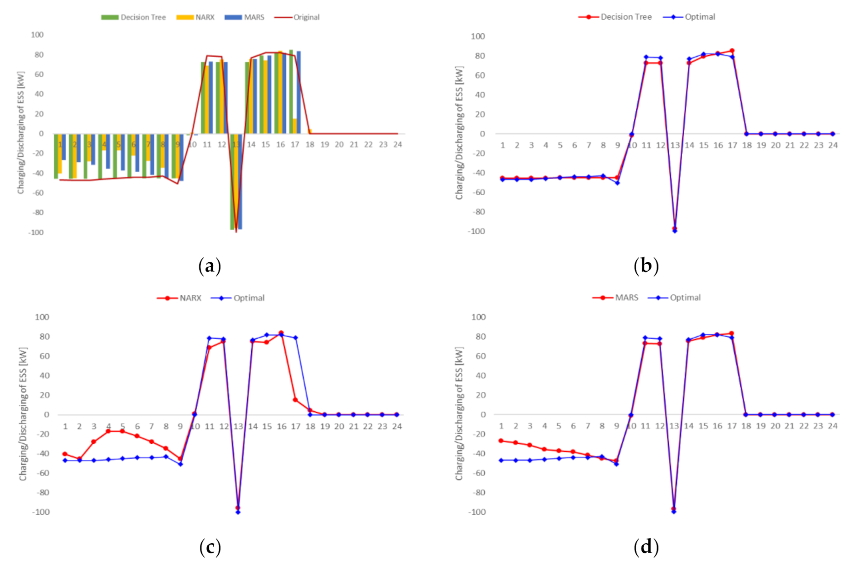
The comparison and analyses of the actual daily ESS charging/discharging, estimated by applying the actual seasonal ESS daily charging/discharging and each technique, are shown in
Figure 10,
Figure 11 and
Figure 12. The actual ESS operation data and the ESS charging/discharging estimated through DT and the actual ESS operation data and the ESS charging/discharging estimated through NARX are shown
Figure 12a–c, showing the actual ESS charging/discharging and the ESS charging/discharging estimated through MARS. As shown in
Table 1 and
Table 2, because the electricity rate time zone and the electricity rate unit price differ for each season according to the load, the ESS operation pattern in winter in
Figure 10 and the ESS operation pattern in spring and summer in
Figure 11 and
Figure 12 differ. Although the unit prices of the electricity rates in spring and summer differ,
Figure 11 and
Figure 12 show the same pattern because the electricity rate time zone is the same.
Figure 10,
Figure 11 and
Figure 12 show that the ESS operation pattern estimated using DT in all seasons is the most similar to the actual ESS operation pattern.
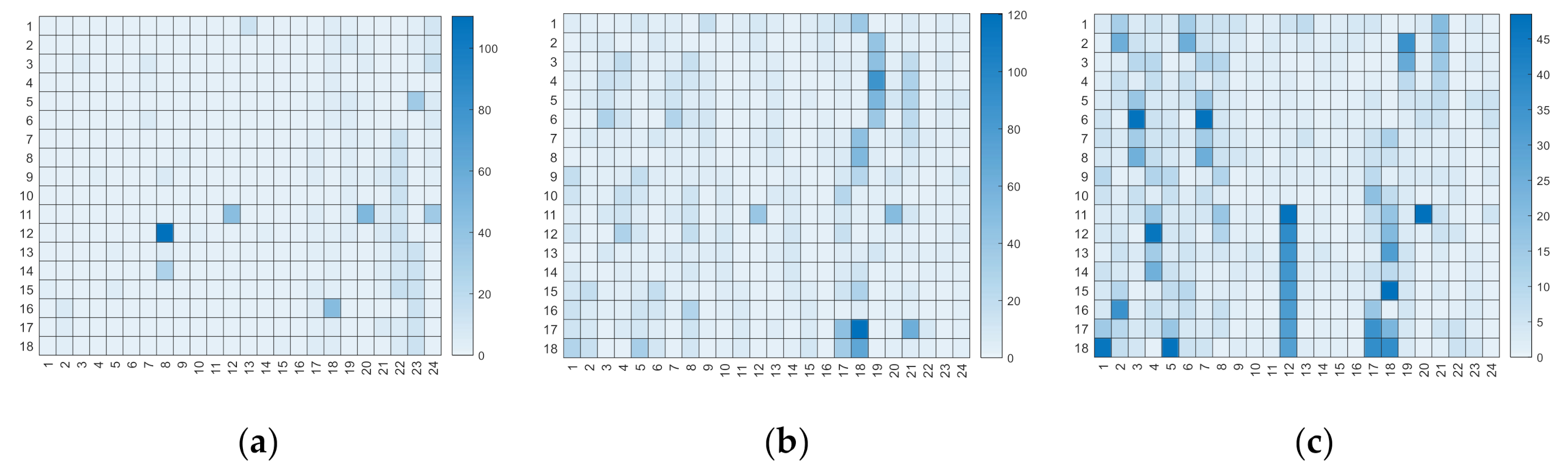
The estimated ESS charging/discharging and the actual value by applying each technique were compared, which is shown in
Figure 13.
Figure 13a indicates that DT had less overall error than the other techniques.
Figure 13b shows that NARX had the highest error value compared with the other techniques, and the error was frequent between 5:00 p.m. and 7:00 p.m.
Figure 13c shows that the error occurred frequently, with the exception of the maximum load time, but the value of the error was small. The maximum value of the error was also the smallest compared with the other techniques.
The results of this case study show that the accuracy of DT is the most similar to the actual ESS operation schedule, and because DT had the highest accuracy, the amount of electricity bill savings did not differ greatly from the actual operation. In contrast, the lowest accuracy of NARX meant that it was different from the actual operation, so it can be found that electricity bills also reduced more than they actually did.
5. Conclusions
This study proposed an optimal charging/discharging scheduling model for application when operating ESS by implementing an actual microgrid in virtual space through a digital twin. A machine learning model was proposed for the purpose of establishing a daily ESS hourly charging/discharging schedule required for microgrid operation, and this was applied to an actual ESS for evaluation. Through the machine learning technique, even if the user does not know the physical characteristics of the ESS, it can be modelled similarly to the actual ESS based on past data, and because the data-based machine learning technique is applied rather than the optimization algorithm, the difficulty of setting the objective function and constraints separately can be solved. The suitability of each model of RMSE and MAE was evaluated, and this was the performance evaluation index of the ESS optimal scheduling model. The savings in electricity bills were calculated and compared with the savings in electricity bills obtained by operating the actual ESS. With regard to the reduction of electricity bills, when the ESS was operated using the proposed machine learning method, more money was saved. Therefore, if the machine learning method most convenient for the user is selected and learned appropriately, the optimal ESS schedule can be sufficiently established with only data, and not physical information. Through the digital twin, the microgrid configuration changed, or various operating algorithms were applied to the virtual space to solve the difficulties experienced in the operation of the existing microgrid and to improve operational efficiency.
If the problem is solved using an optimization-based algorithm, it is possible to solve the problem by deriving the correct objective function rather than past data, but if the problem is solved using machine learning, it is necessary to accumulate historical data for a sufficient period of time. We expect to build an efficient and accurate model through the strategic accumulation of more data in the future. We will continue to collect ESS operational data to verify the accuracy of the model. In addition, we plan to further improve the model performance by changing predictors or parameters for each model and implementing microgrid operation schedules, including PV(Photovoltaic).
Author Contributions
H.-A.P. conceived and designed the experiments; G.B. and J.K. led the project and advised on the whole process of manuscript preparation; H.-C.J. and W.S. analyzed the data; H.-A.P. performed the research and wrote the paper; S.K. provided guidance for the research and revised the paper. All authors have read and agreed to the published version of the manuscript.
Funding
This research was supported by the Korea Electrotechnology Research Institute (KERI) primary research program through the National Research Council of Science and Technology (NST) funded by the Ministry of Science and ICT (MSIT), Republic of Korea (No. 20A01110).
Acknowledgments
This research was supported by the Korea Electrotechnology Research Institute (KERI) primary research program through the National Research Council of Science and Technology (NST) funded by the Ministry of Science and ICT (MSIT), Republic of Korea (No. 20A01110).
Conflicts of Interest
The authors declare no conflict of interest.
References
- Korea Energy Agency. Available online: www.energy.or.kr (accessed on 20 October 2020).
- Soroudi, A.; Siano, P.; Keane, A. Optimal DR and ESS scheduling for distribution losses payments minimization under electricity price uncertainty. IEEE Trans. Smart Grid 2015, 7, 261–272. [Google Scholar] [CrossRef]
- Choi, S.; Min, S.W. Optimal scheduling and operation of the ESS for prosumer market environment in grid-connected industrial complex. IEEE Trans. Ind. Appl. 2018, 54, 1949–1957. [Google Scholar] [CrossRef]
- Gonzales-Zurita, Ó.; Clairand, J.M.; Peñalvo-López, E.; Escrivá-Escrivá, G. Review on Multi-Objective Control Strategies for Distributed Generation on Inverter-Based Microgrids. Energies 2020, 13, 3483. [Google Scholar] [CrossRef]
- Park, M.; Kim, J.; Won, D.; Kim, J. Development of a two-stage ESS-scheduling model for cost minimization using machine learning-based load prediction techniques. Processes 2019, 7, 370. [Google Scholar] [CrossRef]
- Morais, H.; Kádár, P.; Faria, P.; Vale, Z.A.; Khodr, H.M. Optimal scheduling of a renewable micro-grid in an isolated load area using mixed-integer linear programming. Renew. Energy 2010, 35, 151–156. [Google Scholar] [CrossRef]
- Yuan, X.; Wang, L.; Yuan, Y. Application of enhanced PSO approach to optimal scheduling of hydro system. Energy Convers. Manag. 2008, 49, 2966–2972. [Google Scholar] [CrossRef]
- Chen, C.L. Simulated annealing-based optimal wind-thermal coordination scheduling. IET Gener. Transm. Distrib. 2007, 1, 447–455. [Google Scholar] [CrossRef]
- Grieves, M.; Vickers, J. Digital twin: Mitigating unpredictable, undesirable emergent behavior in complex systems. In Transdisciplinary Perspectives on Complex Systems; Springer: Cham, Switzerland, 2017; pp. 85–113. [Google Scholar]
- Grieves, M.W. Virtually intelligent product systems: Digital and physical twins. Complex Syst. Eng. Theory Pract. 2019, 175–200. [Google Scholar] [CrossRef]
- Jones, D.; Snider, C.; Nassehi, A.; Yon, J.; Hicks, B. Characterising the Digital Twin: A systematic literature review. CIRP J. Manuf. Sci. Technol. 2020, 29, 36–52. [Google Scholar] [CrossRef]
- Uhlemann, T.H.J.; Schock, C.; Lehmann, C.; Freiberger, S.; Steinhilper, R. The digital twin: Demonstrating the potential of real time data acquisition in production systems. Procedia Manuf. 2017, 9, 113–120. [Google Scholar] [CrossRef]
- Saad, A.; Faddel, S.; Mohammed, O. IoT-Based Digital Twin for Energy Cyber-Physical Systems: Design and Implementation. Energies 2020, 13, 4762. [Google Scholar] [CrossRef]
- Madni, A.M.; Madni, C.C.; Lucero, S.D. Leveraging digital twin technology in model-based systems engineering. Systems 2019, 7, 7. [Google Scholar] [CrossRef]
- Negri, E.; Fumagalli, L.; Macchi, M. A review of the roles of digital twin in cps-based production systems. Procedia Manuf. 2017, 11, 939–948. [Google Scholar] [CrossRef]
- Samuel, A.L. Some studies in machine learning using the game of checkers. IBM J. Res. Dev. 1959, 3, 210–229. [Google Scholar] [CrossRef]
- Samuel, A.L. Some studies in machine learning using the game of checkers. II—Recent progress. Annu. Rev. Autom. Program. 1969, 6, 1–36. [Google Scholar] [CrossRef]
- Michie, D.; Spiegelhalter, D.J.; Taylor, C.C. Machine learning. Neural Stat. Classif. 1994, 13, 1–298. [Google Scholar]
- Kotsiantis, S.B.; Zaharakis, I.; Pintelas, P. Supervised machine learning: A review of classification techniques. Emerg. Artif. Intell. Appl. Comput. Eng. 2007, 160, 3–24. [Google Scholar]
- Längkvist, M.; Karlsson, L.; Loutfi, A. A review of unsupervised feature learning and deep learning for time-series modeling. Pattern Recognit. Lett. 2014, 42, 11–24. [Google Scholar] [CrossRef]
- Sutton, R.S.; Barto, A.G. Reinforcement Learning: An Introduction, 2nd ed.; MIT Press: Cambridge, UK, 2018; Volume 13, pp. 1–525. [Google Scholar]
- Rudin, C.; Waltz, D.; Anderson, R.N.; Boulanger, A.; Salleb-Aouissi, A.; Chow, M.; Isaac, D.F. Machine learning for the New York City power grid. IEEE Trans. Pattern Anal. Mach. Intell. 2011, 34, 328–345. [Google Scholar] [CrossRef]
- Sunyong Kim; Hyuk Lim. Reinforcement Learning Based Energy Management Algorithm for Smart Energy Building. Energies 2018, 11, 2010. [Google Scholar] [CrossRef]
- Diaconescu, E. The use of NARX Neural Networks to predict Chaotic Time Series. Wseas Trans. Comput. Res. 2008, 3, 182–191. [Google Scholar]
- James, G.; Witten, D.; Hastie, T.; Tibshirani, R. An Introduction to Statistical Learning; Springer: New York, NY, USA, 2013. [Google Scholar]
- Friedman, J.H. Multivariate adaptive regression splines. Ann. Stat. 1991, 19, 1–67. [Google Scholar] [CrossRef]
- Kim, S.K.; Cho, K.H.; Kim, J.Y.; Byeon, G.S. Field study on operational performance and economics of lithium-polymer and lead-acid battery systems for consumer load management. Renew. Sustain. Energy Rev. 2019, 113, 109234. [Google Scholar] [CrossRef]
- Korea Electric Power Corporation, KEPCO Electric Rates Table. Available online: www.kepco.co.kr (accessed on 20 October 2020).
Figure 1.
Digital twin concept for microgrid.
Figure 1.
Digital twin concept for microgrid.
Figure 2.
Types of machine learning.
Figure 2.
Types of machine learning.
Figure 3.
Architecture of NARX networks.
Figure 3.
Architecture of NARX networks.
Figure 4.
Optimal scheduling process for energy storage system in field [
27].
Figure 4.
Optimal scheduling process for energy storage system in field [
27].
Figure 5.
Energy storage system under field operation: battery racks (left), inverter and transformer (right).
Figure 5.
Energy storage system under field operation: battery racks (left), inverter and transformer (right).
Figure 6.
Real operating data of energy storage system (November 2019–July 2020).
Figure 6.
Real operating data of energy storage system (November 2019–July 2020).
Figure 7.
Flowchart of the proposed ESS optimal scheduling using machine learning.
Figure 7.
Flowchart of the proposed ESS optimal scheduling using machine learning.
Figure 8.
Chart of seasonal savings of electricity rate with Machine learning algorithms.
Figure 8.
Chart of seasonal savings of electricity rate with Machine learning algorithms.
Figure 9.
Scatter plot of all simulation results: (a) comparison of original data and proposed output with decision tree, (b) comparison of original data and proposed output with NARX, (c) comparison of original data and proposed output with MARS.
Figure 9.
Scatter plot of all simulation results: (a) comparison of original data and proposed output with decision tree, (b) comparison of original data and proposed output with NARX, (c) comparison of original data and proposed output with MARS.
Figure 10.
(a) Optimal schedule of ESS for minimization of operation cost at winter, (b) real and simulation results with DT, (c) real and simulation results with NARX, (d) real and simulation results with MARS.
Figure 10.
(a) Optimal schedule of ESS for minimization of operation cost at winter, (b) real and simulation results with DT, (c) real and simulation results with NARX, (d) real and simulation results with MARS.
Figure 11.
(a) Optimal schedule of ESS for minimization of operation cost at spring, (b) real and simulation results with DT, (c) real and simulation results with NARX, (d) real and simulation results with MARS.
Figure 11.
(a) Optimal schedule of ESS for minimization of operation cost at spring, (b) real and simulation results with DT, (c) real and simulation results with NARX, (d) real and simulation results with MARS.
Figure 12.
(a) Optimal schedule of ESS for minimization of operation cost at summer, (b) real and simulation results with DT, (c) real and simulation results with NARX, (d) real and simulation results with MARS.
Figure 12.
(a) Optimal schedule of ESS for minimization of operation cost at summer, (b) real and simulation results with DT, (c) real and simulation results with NARX, (d) real and simulation results with MARS.
Figure 13.
Comparison of error for simulation results: (a) error of simulation results with decision tree, (b) error of simulation results with NARX, (c) error of simulation results with MARS.
Figure 13.
Comparison of error for simulation results: (a) error of simulation results with decision tree, (b) error of simulation results with NARX, (c) error of simulation results with MARS.
Table 1.
Time Zones for off-Peak, mid-peak, peak load.
Table 1.
Time Zones for off-Peak, mid-peak, peak load.
| | Winter | Spring | Summer |
|---|
| Off-Peak Load | 23:00–09:00 | 23:00–09:00 | 23:00–09:00 |
| Mid-Peak Load | 09:00–10:00 | 09:00–10:00 | 09:00–10:00 |
| 12:00–17:00 | 12:00–13:00 | 12:00–13:00 |
| 20:00–22:00 | 17:00–23:00 | 17:00–23:00 |
| Peak Load | 10:00–12:00
17:00–20:00
22:00–23:00 | 10:00–12:00
13:00–17:00 | 10:00–12:00
13:00–17:00 |
Table 2.
Electric rates of TOU tariff for industrial customers.
Table 2.
Electric rates of TOU tariff for industrial customers.
| | Winter | Spring | Summer |
|---|
| Off-Peak Load (KRW/kW) | 63.1 | 56.1 | 56.1 |
| Mid-Peak Load (KRW/kW) | 109.2 | 78.6 | 109.0 |
| Peak Load (KRW/kW) | 166.7 | 109.3 | 191.1 |
Table 3.
NARX Network Conditions.
Table 3.
NARX Network Conditions.
| Setting List | Setting Value |
|---|
| Time delay | 2 |
| Feedback delay | 1:2 |
| Hidden layer size | 10 |
| Training dataset | 720 samplings |
| Validation dataset | 144 samplings |
| Testing dataset | 144 samplings |
| Activate function | Sigmoid function |
| Training method | Levenberg–Marquardt backpropagation |
| Validation checks | 100 |
Table 4.
Savings of Electricity Rate (KRW).
Table 4.
Savings of Electricity Rate (KRW).
| Season | Optimal | Decision Tree | NARX | MARS |
|---|
| Winter | 359,899 | 337,791 | 375,512 | 362,547 |
| Spring | 122,658 | 128,252 | 140,097 | 107,447 |
| Summer | 334,694 | 335,134 | 305,090 | 330,103 |
| Total | 817,251 | 801,177 | 820,699 | 800,097 |
Table 5.
Accuracy of model based on test data.
Table 5.
Accuracy of model based on test data.
| Season | RMSE | MAE |
|---|
| Decision Tree | NARX | MARS | Decision Tree | NARX | MARS |
|---|
| Winter | 9.56 | 9.46 | 12.07 | 1.60 | 6.70 | 7.39 |
| Spring | 3.90 | 5.41 | 8.61 | 0.68 | 3.19 | 3.35 |
| Summer | 8.52 | 19.61 | 10.61 | 4.33 | 9.78 | 5.37 |
| Publisher’s Note: MDPI stays neutral with regard to jurisdictional claims in published maps and institutional affiliations. |
© 2020 by the authors. Licensee MDPI, Basel, Switzerland. This article is an open access article distributed under the terms and conditions of the Creative Commons Attribution (CC BY) license (http://creativecommons.org/licenses/by/4.0/).


