Representative Environmental Condition for Fatigue Analysis of Offshore Jacket Substructure

Abstract

The 20-year cumulative fatigue damage of an offshore jacket substructure was estimated under the long-term local environmental conditions in the Taiwan Strait. Because of the nonlinearity of wave load for slender members of the structure, time-domain simulations of the dynamic finite element model were conducted for each sea state. By utilizing the Dirlik method to process the stress signals, the fatigue damages of joints were computed. Concerning the computational time, we propose a probability-based method of using a representative combination of environmental conditions in this study, which can considerably reduce the required number of evaluations prior to determining fatigue damage, thereby improving the process of preliminary design. The results show that only three sea states among 120 can represent 28% of the average damage ratio, and up to 17 sea states fully resolved the fatigue life.

1. Introduction

According to statistical reports, the global wind turbine installation capacity reached 651 GW by the end of 2019 [1]. This value is predicted to increase to 840.9 GW by 2022 [2]. Offshore wind turbines are crucial for withstanding the cyclic load exerted by winds and waves in the ocean. Moreover, structures in the sea are susceptible to corrosion damage. In recent years, large-scale wind turbine structures have been used. The aforementioned information reveals that structural problems are crucial. Moreover, earthquakes, typhoons, ocean currents, high temperatures, and high humidity pose tremendous threats to the strength of the substructures, especially in Taiwan. Damages occur in various offshore scenarios—for example, ultimate (extreme) load, fatigue, accidental ship impact, or soil liquefaction. Among them, fatigue damage occurs slowly and is difficult to detect due to several sub-issues: marine growth, corrosion, vibrations in vortex shedding, and imperfection of materials. In jacket substructures, the most damage is observed in the splash zone of a tower and joints of substructures [3]. Tubular joint connections present in jacket substructures are subject to approximately 109 load cycles during their designed lifetime of 20 years [4] and thus are critical connections that may undergo fatigue failure.

On offshore bottom-fixed wind turbines, fatigues induced by wind and wave load fluctuations are usually addressed independently by turbine manufacturer and construction contractor, respectively, followed by a superposition or load coupling of them on the substructure. The time-consuming iteration across the wind–wave interface and the communication overhead slow down the design process of the substructure. This shortcoming demonstrates the necessity of boosting fatigue assessments. Fatigue analysis methods can be categorized into two major simulation methods: time-domain (TD) and frequency-domain (FD). For nonlinear systems, the TD method is more accurate than the FD method. However, computations for acquiring a solution by using the TD method are expensive [5]. Conversely, the FD method is better than the TD method in terms of calculation time. Thus, the FD method has received widespread attention. The FD method assumes that highly nonlinear systems respond linearly to given inputs [6] and employs the relationship between the load and the structure response to provide a reaction amplitude operator, or a transfer function, to which a power spectrum is applied. This fatigue assessment approach has been used for large, complex structures, such as ship structures [7], structures in oil and gas industries [8], and offshore wind turbines [9].

Because of the nonlinearity of wave loads in stringent sea states, the FD method could underestimate the stress fluctuations, and use of the TD method is inevitable. The feasible approaches that can be used to reduce the large amount of time in TD fatigue analyses are reducing the number of analysis sets or finding a set of representative sea states for fatigue damage estimation instead of considering all the environmental conditions. Chian et al. used a Monte Carlo sampling method to estimate fatigue damage, and the test result yielded the same error level for grids (2443 iterations required) after 1437 iterations [10]. Dong et al. considered the same direction of winds and waves to reduce the computational effort involved in estimating fatigue damage and identified the representative environmental condition in the North Sea corresponding to the maximum contribution to fatigue damage [4]. Baarholm et al. [11] estimated hull girder loads in ships by distinguishing sea states contributing to nonlinearity solved via a TD method, and other sea states are treated by a spectral FD analysis. The present study was conducted to determine the representative environmental conditions with the highest benefit and reduce the number of analysis sets required to reduce the analysis time.

This paper is organized as follows. Section 2 presents the computational model and the fatigue life assessment method for jacket structures under short-term meteorological and oceanographic statistics, abbreviated as metocean conditions in the following content. These statistics basically include wind speed and sea state. Section 3 describes the long-term metocean conditions statistics and provides the related probability distribution models. In this section, we formulate the characteristics of accumulated fatigue damage and present three methods for selecting representative sea states. In Section 4, the structural fatigue under each metocean condition is analyzed using the proposed model. The obtained fatigue information was compared with that obtained using other selection methods. The quantitative measures of representativeness were evaluated for the fatigue of each structural joint and each metocean condition. Conclusions are provided in Section 5.

2. Fatigue Life Assessment

The procedure of fatigue assessment is demonstrated in Figure 1. This section presents the computational model and the finite element analysis (FEA) for jacket structures for each sea state, corresponding to the orange boxes. This is the most time-consuming part in terms of computation. A representative selection method, the grey box, can limit the loop iterations in FEA.

2.1. Numerical Model of Jacket Substructure

A jacket X-type substructure made of steel, established at a depth of 50 m [12], was selected and built in SACS software (Bentley Systems Inc., Exton, PA, USA), a design and analysis software package for offshore structures. Because no relevant information about the pile soil was available, the bottom end of the substructure was set as a fixed end in the boundary condition. Detailed final geometrical information is listed in Appendix A of this study. The nature frequency of this target substructure is 0.32 Hz, which is considered as a stiff-stiff design, compared to given waves and wind fluctuations. Structural damping 1% is considered in the dynamic analysis [13].

According to the recommendation of the International Electrotechnical Commission 61400-3 (IEC 61400-3) [14], the Pierson–Moskowitz spectrum was used for conducting fatigue analysis, and the environmental spectrum was developed according to the model Equation (1).

$${\mathrm{S}}_{PM}\left(f\right)=\frac{5{\mathrm{H}}_s{}^2{\mathrm{T}}_p}{16}\frac{1}{ f^5 }\exp \left[-\frac{5}{4}{\left(f\right)}^{-4}\right],$$

(1)

where H_s is the significant wave height and T_p is the peak wave period. The power spectral densities of ocean waves describe the wave heights of individual waves at different frequencies. Then, the time history of an irregular sea state can be reconstructed by superposing many component waves, which follow a presented power spectral density equation and random phases [15]. A preload step of 150 s was applied as a ramp load on the structure, and then 600 s simulation time was performed under each sea state. Stress signals were taken in the later 600 s for fatigue analysis.

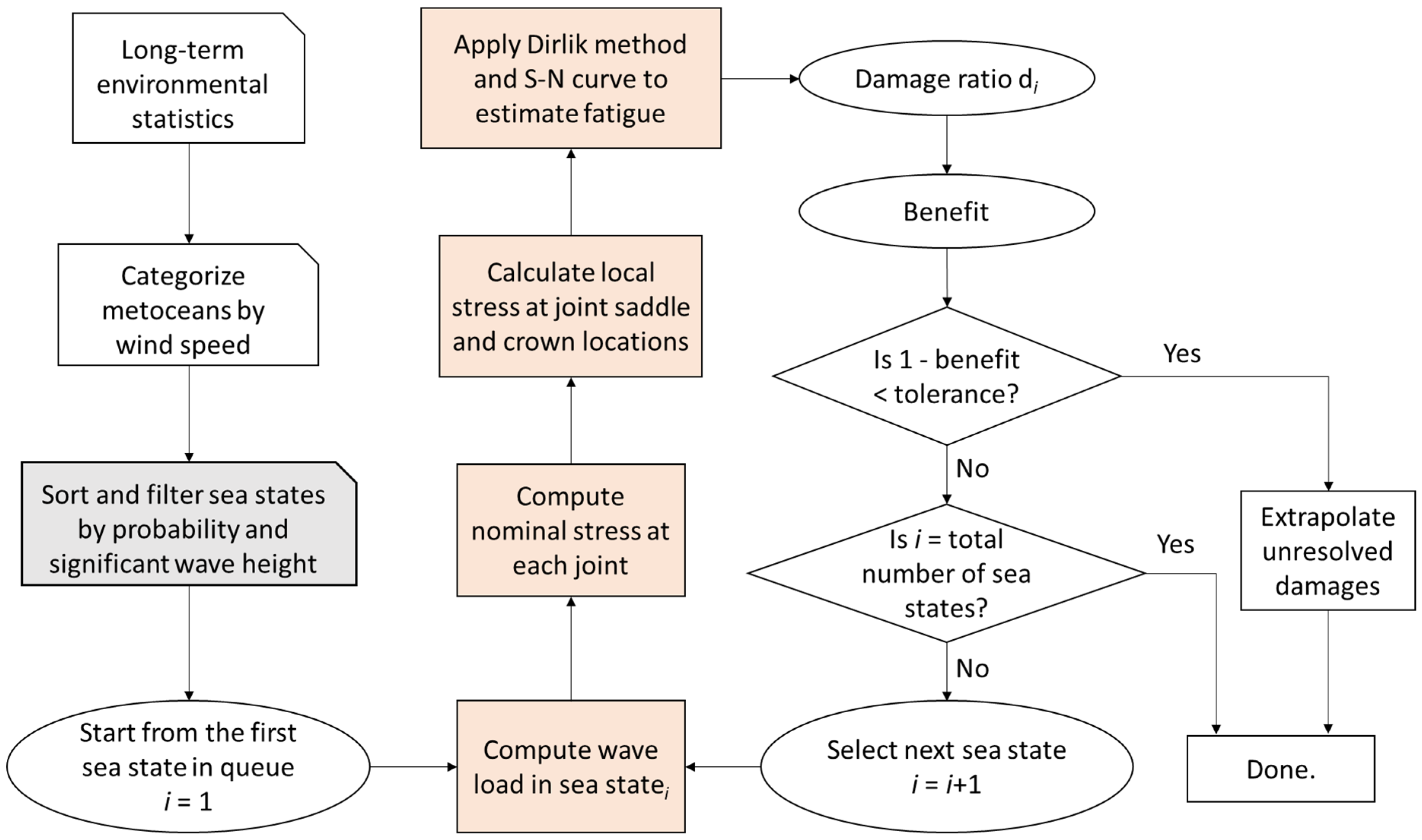
2.2. Fatigue Damage Assessment

Six joints were observed in the substructures in this study; these joints were selected to investigate the relationship between the degree of damage of a joint and the distance from the seabed to a column, as per Figure 2a. Three structural response stress signals of the axial force (FA), in-plane bending (IPB), and out-of-plane bending (OPB) were selected among the six observation points that pertain to the maximum damage hotspots.

Weld joints are critical connections based on the experience of the offshore industry. Therefore, the hotspot stress method, recommended by Det Norske Veritas Germanischer Lloyd (DNV GL) [16], was implemented in this study for evaluating the fatigue damage at the tubular joints. The hotspot stress was evaluated at eight spots around the circumference of the intersection of joints; see Figure 2b. An increase in the stress effect can be considered by the hotspot stress range through the stress concentration factor (SCF) to modify the nominal stress in Equation (2), where σ_nominal is the stress at joint simulated by FEA.

$${\mathsf{\sigma }}_{\mathrm{hot} \mathrm{spot}}=\mathrm{SCF}\times {\mathsf{\sigma }}_{\mathrm{nominal}}$$

(2)

Then, by assuming that a structure is in a sea state in which the time-domain load signal is a stable random Gaussian process, Dirlik [17] used the probability density function (PDF) of Gaussian, Rayleigh, and exponential distribution combined stress spectra to estimate randomness. Most related studies recommend the use of the Dirlik method in the frequency domain [18] because the obtained estimation results are very close to the Rainflow counting method in the time domain [9]. Then, the basic design of the S–N curve is applied, as per Equation (3) [16], where N represents the number of cycles to failure in the stress range, ∆σ is the stress range, and $\overline{a}$ and m are constants that depend on the material and the environmental conditions, respectively.

$$\log N=\log \overline{a} - m\log \left(\mathsf{\Delta }\mathsf{\sigma }\right),$$

(3)

where empirical studies give m = 3.0 and $\overline{a}$ = 12.18 if N ≤ 1.8 × 10⁶, or m = 5.0 and $\overline{a}$ = 16.13 if N > 1.8 × 10⁶. Three types of S–N curves for the tubular joints (known as T-curves) under different environments were presented in [16] for air, seawater with cathodic protection, and seawater to enable free corrosion. The T-curve contains three levels based on the material grade, and the material used in this study pertains to the B-level condition.

The Dirlik method was combined with a selected S–N curve to determine the fatigue damage. Then, fatigue damage calculation was conducted using the widely used Palmgren–Miner linear damage theory [16,19]. D_g is the accumulated fatigue damage that is expressed in Equation (4). The formula reveals that fatigue damage occurs when D_g is greater than 1. Equation (4) provides an explicit relationship between the stress range and the damage, which is used in the later accumulation calculation.

$$D_g=\Sigma \frac{n_i}{N_i}=\Sigma \left(\frac{n_i}{\overline{a}}\times \mathsf{\Delta }{\sigma }_i{}^m\right)$$

(4)

Finally, the maximum fatigue damage in the eight spots of each joint as mentioned can be calculated by considering the stress concentration factor and estimating the damage of the jacket substructure for each joint position for 20 years, as per Figure 3. Taking the most common sea state [H_s,T_p] = [0.5 m, 6 s], for example, red color blocks mark the higher fatigue damage values for each joint, and green color blocks mark the lower fatigue damage values.

3. Long-Term Metocean Statistics

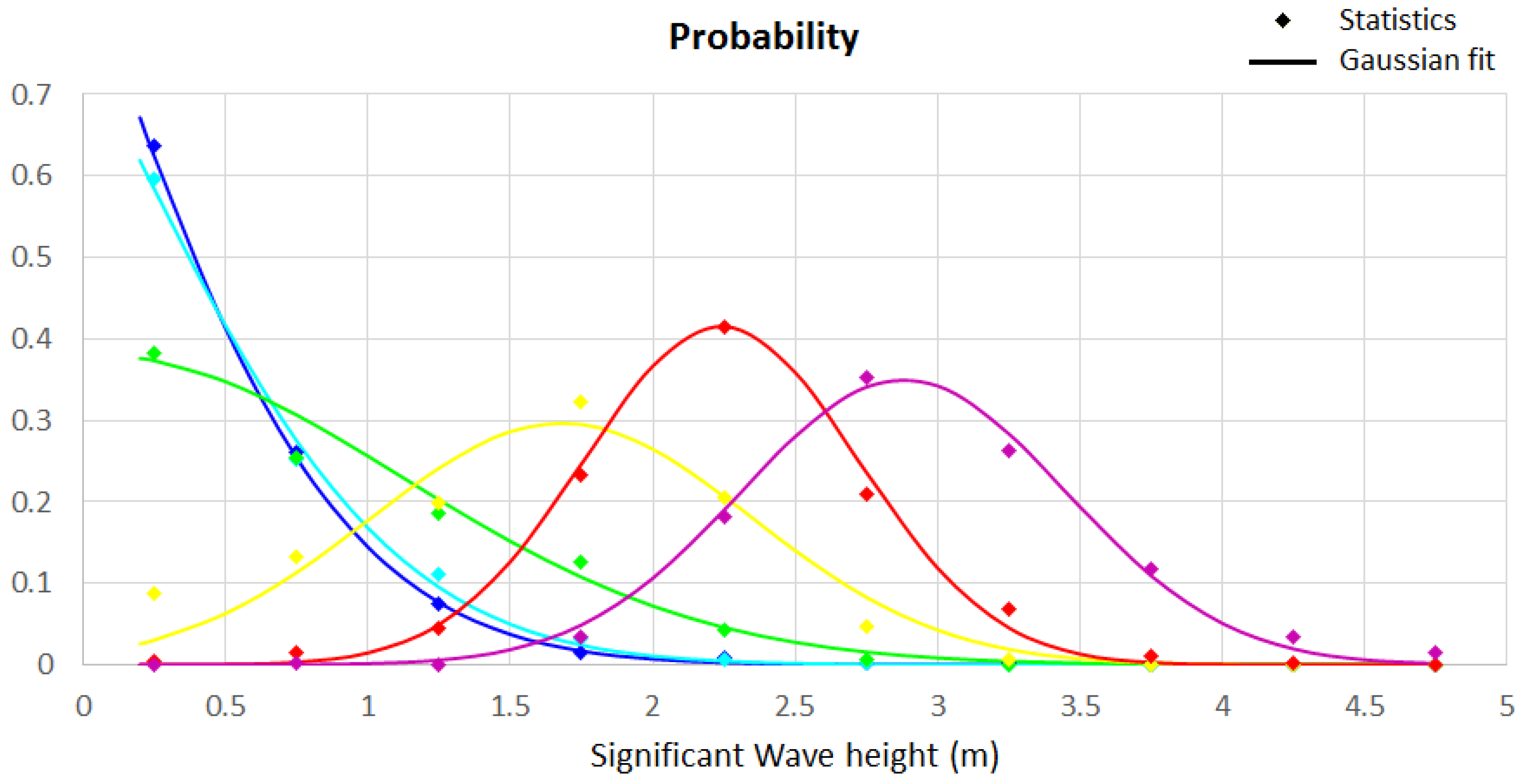
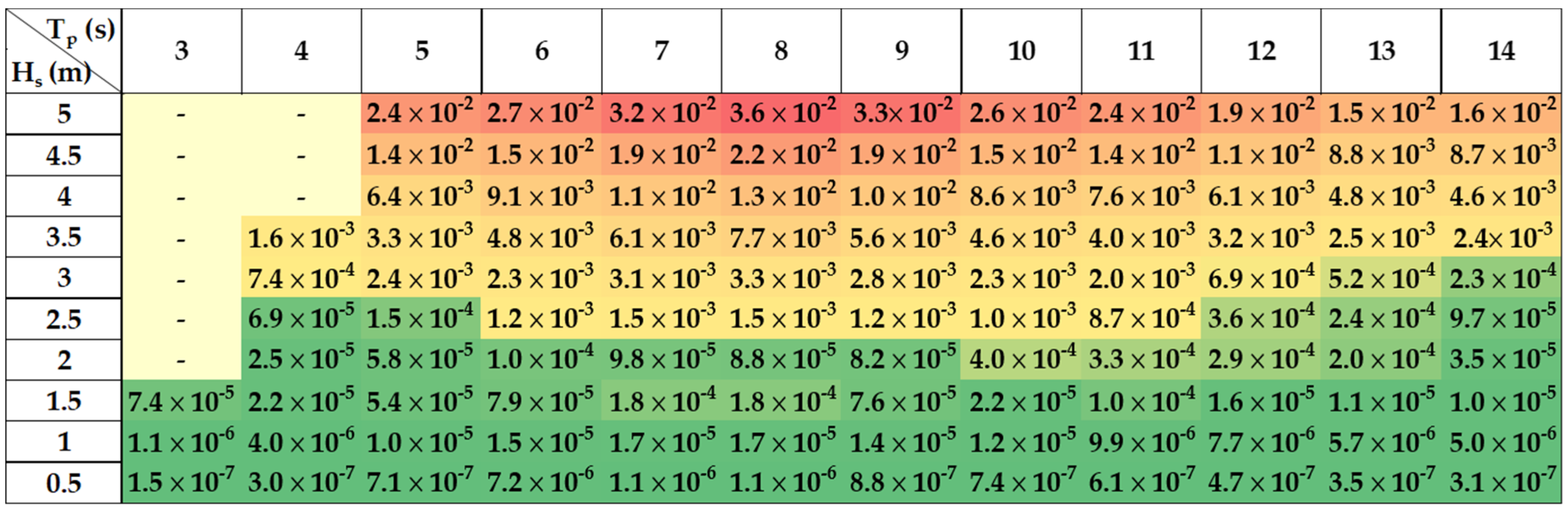
3.1. Wave Scatter Diagram

The long-term environmental statistics were based on a preliminary site survey that was conducted from December 1991 to August 1999 at the west sea area in Taiwan. The average wind speed is classified into six bins from 0 to 30 m/s, with an interval of 5 m/s, and the wave height is categorized into ten sections from 0 to 5 m, with an interval of 0.5 m. The wave period is divided into twelve bins from 3 to 15 s, with an interval of 1 s. The data include 120 types of sea state, and the total probability is 100%. The sea states are further categorized into six metocean conditions based on the wind speed. The aforementioned categorization is essential not only for the following derivation of the statistics of sea states but also for the wind-induced fatigue because the superstructures or power turbines are usually dependent on the wind speed. The wind force data can be separately incorporated in the structural model through external sources [9]. However, such a method is beyond the scope of the present study and is not considered for that focusing on the wave-induced fatigue and the representativeness of sea states. The occurrence probabilities of the wind speed ranges in the report are referred to as Metocean 1 to 6 (Figure 4). The detail of the highest probability environment for the six wind speed ranges is listed in

Table 1. Highest probability of the six wind speed ranges.

Metocean	1	2	3	4	5	6
Wind speed (m/s)	0–5	5–10	10–15	15–20	20–25	25+
Wave height (m)	0.5	0.5	0.5	2.0	2.5	3.0
Wave period (s)	6	6	6	6	6	7
Highest Probability	32%	30%	18%	20%	22%	17%

. Due to lack of the information on wave direction, these metocean conditions are set as unidirectional, aligned with the orientation of the foundation. This simplification is based on the notion that the normal facing against the load usually imposes the largest amount of energy on the structure, which is considered the essential load case in a preliminary design. Multi-directional and wind-wave misalignment load cases could be evaluated in a full analysis.

The probability distribution against significant wave height is assumed to be truncated normal distribution. To confirm, we summed the probabilities of all the T_p values for each wave height to obtain the probability distribution of significant wave heights for each metocean condition. The probability distribution is presented in

Table 2. Probability distribution (%) of significant wave heights under the six metocean conditions. (SD represents Standard Deviation).

Metocean		1	2	3	4	5	6
Wind speed (m/s)		0–5	5–10	10–15	15–20	20–25	25+
Significant wave height (m)	5	0.0	0.0	0.0	0.0	0.0	1.4
	4.5	0.0	0.0	0.0	0.0	0.1	3.5
	4	0.0	0.0	0.0	0.0	1.1	11.7
	3.5	0.2	0.0	0.1	0.7	6.8	26.3
	3	0.2	0.1	0.6	4.6	20.9	35.2
	2.5	0.8	0.6	4.3	20.5	41.5	18.1
	2	1.6	3.3	12.7	32.2	23.2	3.5
	1.5	7.5	11.1	18.6	19.9	4.5	0.0
	1	26.0	25.3	25.4	13.3	1.5	0.2
	0.5	63.7	59.5	38.3	8.7	0.4	0.0
Gaussian Fit—Mean		−0.99	−0.72	0.05	1.68	2.24	2.88
Gaussian Fit—SD		0.91	0.9	1.07	0.67	0.48	0.57

. The probability distributions were fitted with normal distributions, drawn in Figure 5, where the mean values and standard deviations are listed at the bottom of Table 2.

3.2. Cumulative Fatigue Damage

In this study, a total of 120 environmental sea states were analyzed for the target jacket substructure. The wave load evaluation conducted on slender offshore structures commonly utilizes the Morison equation, in which the inertia term is proportional to the wave height and the drag term is proportional to the square of the wave height [20]. We could infer that the wave load is proportional to the wave height of an exponent α, which is between one and two based on the contributions of the two aforementioned terms. A wave force regime stated in this reference reveals that the higher a wave is, the higher the domination of the drag term is (that is, α approaches two and becomes nonlinear).

For the structural response, the stress range is also positively correlated to the wave load range, which is proportional to the wave height of α. Then, by combining the Dirlik method with the exponent of wave load, the cumulative damage is expressed in terms of the wave height power in Equation (5), where f is a constant multiplier.

$$D_g=\Sigma \left(\frac{n_i}{\overline{a}}\times \mathsf{\Delta }{\sigma }_i{}^m\right)=f\times H_s{}^{\alpha m}$$

(5)

Figure 6 displays the fatigue cumulative damage values of A-3 joint R hotspot in the 120 sea states for 20 years. If the damage value is 1, then the joint position is considered to be damaged due to fatigue. The same color gradients were applied to the blocks to mark the corresponding damage values. A detailed description of other hotspots is provided in Appendix B. These figures indicate that the wave height is the dominant factor affecting the joint damages. To validate the above expression, the cumulative damages of the six joints were fitted by the least square method. The fitting parameters are depicted in

Table 3. Fitting parameters for fatigue damage at joints.

Joint	Multiplier f	Exponent α*m
A-3	2.5 × 10−5	4.4
C-3	3.5 × 10−5	4.7
B-4	1.3 × 10−5	4.5
D-4	1.0 × 10−5	4.7
A-5	2.5 × 10−6	5.0
C-5	2.0 × 10−6	4.7

and Figure 7. The multiplier is larger for the lower layers of the jacket. Thus, higher fatigue damage is observed in the joints closer to the seabed. The exponent α*m is between 4.5 and 5, and this value roughly complies with the slope of the S–N curve.

3.3. Representative Selection Method

The overall cumulative damage D_natural represents the total damage of all sea states, which is the product of the summation of probability and its corresponding cumulative damage. For each probability distribution under Metocean 1–6, D_natural is computed at each joint, as per

Table 4. D_nature at each joint under each metocean condition. The color gradients from light blue to pale red classify the values in ascending order.

Metocean	1	2	3	4	5	6
A-3	4.6 × 10−5	4.1 × 10−5	1.2 × 10−4	5.1 × 10−4	1.8 × 10−3	5.3 × 10−3
C-3	7.4 × 10−5	6.7 × 10−5	2.0 × 10−4	8.8 × 10−4	3.1 × 10−3	9.4 × 10−3
B-4	2.0 × 10−5	2.0 × 10−5	6.3 × 10−5	2.8 × 10−4	9.5 × 10−4	2.8 × 10−3
D-4	2.1 × 10−5	2.1 × 10−5	6.7 × 10−5	3.0 × 10−4	1.0 × 10−3	3.1 × 10−3
A-5	1.4 × 10−6	1.5 × 10−6	5.2 × 10−6	2.5 × 10−5	8.1 × 10−5	2.4 × 10−4
C-5	9.6 × 10−7	1.1 × 10−6	3.6 × 10−6	1.7 × 10−5	5.3 × 10−5	1.4 × 10−4

. Then, the damage ratio of partial damage of choice from sea states is defined as D_part/D_natural. The damage ratio is a measure of how much a selected sea state represents the overall damage. Because there are six metocean conditions in the study, the average damage value is the average of the six damage ratios of each metocean condition. Moreover, the probability value is the sum of the occurrence probability of the selected sea states. The benefit value represents the marginal damage ratio due to the occurrence probability per 1%. The total benefit, given by Equation (6), is calculated from the average damage ratio of the six metocean conditions and the occurrence probability and represents the damage ratio effect due to the probability of occurrence per 1%.

Following the damage ratio as defined, one seeks high representativeness either through the sea states of high probabilities or of causing high damage. Since both are in terms of wave height, the former follows a Gaussian function and the latter follows an exponential function; the probability distribution quickly suppresses the damage in the decreasing power of H_s² to the increasing power of $\log H_s$ when the wave height increases. This crucial characteristic implies that the damage ratio follows the probability function more than the damage function. Figure 8 presents the probabilities of Metocean 2 and 5 in red-colored curves. The cumulative damage at joint A3 is provided in black-colored curves, and the damage ratios are represented by green-colored curves. The figure indicates that the damage ratio peak lies on the right side of the probability peak because the damage function puts a higher weight on high waves. The two peaks deviate less in the high wave condition. Thus, a conservative estimate of the highest damage ratio is obtained from the most probable sea state corresponding to the higher wave in the absence of damage information.

$$total benefit= \frac{{\sum }_{i=1}^{numbers of metocean }{\mathrm{Average}}_i}{{\sum }_{i=1}^{numbers of metocean }{\mathrm{Probability}}_i}$$

(6)

Based on the characteristics of probability and damage in terms of wave height, we proposed a simple sorting of sea states by probability (abbreviated as Pr type), as described below. The first sea state is the most probable sea state P_max. Moreover, from the Gaussian distributions of wave scatter diagrams, more probable sea states locate around P_max. So, another selection method is by the neighborhood around P_max, abbreviated as Nb type.

(1)

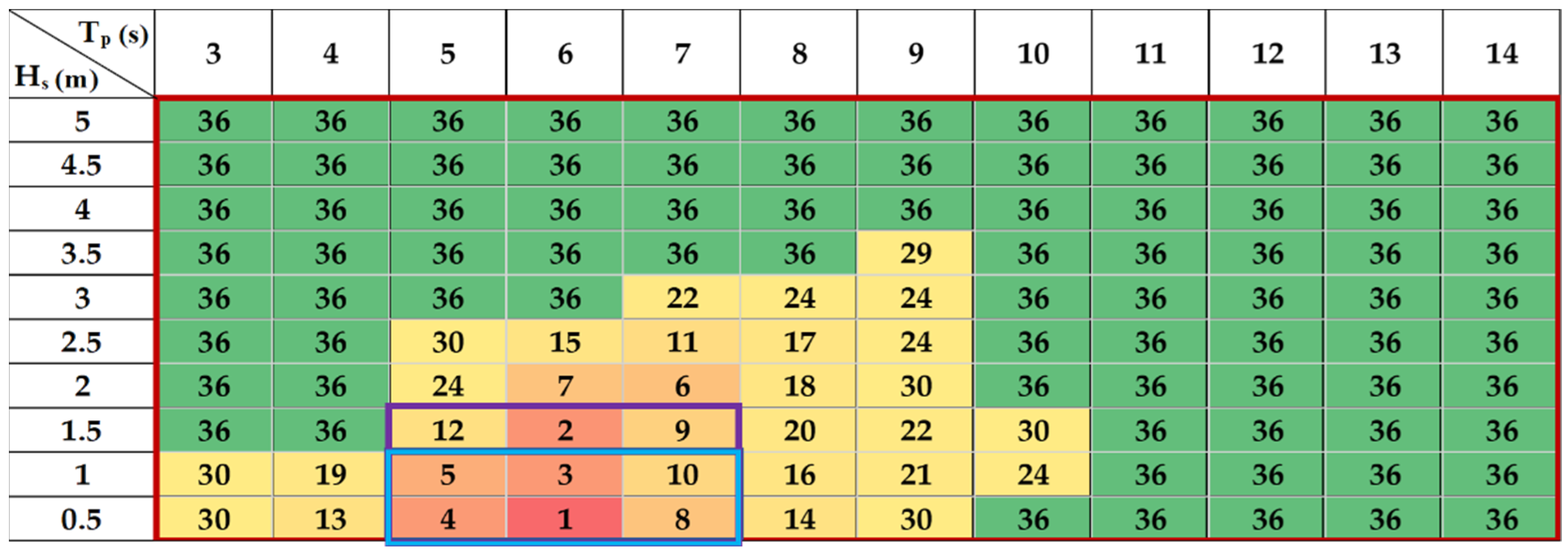
Probability type (Pr): the algorithm of the probability type is selected on the basis of the rank of probability when the probability distribution is monotonically decreasing. This method can mitigate the problem caused by local peaks in the probability distribution of the raw statistics. The total number M of selected sea states is denoted Pr-M in the following discussion—for example, Pr-6 and Pr-9. Since high waves contribute to higher damage, the sea states with a lower wave height than the sea states at the most probable sea state P_max are omitted, denoted Pr-6U and Pr-9U. Moreover, when the same probability occurs in the same wave period, the condition of higher wave height should be selected. When the same probability occurs at the same wave height, the condition of the smaller wave period should be selected. The numbers in Figure 9a are ranked according to the probability and the figure displays the selected range of environmental conditions in the Metocean 5. The selected sea states are detailed in Appendix C.

(2)

Neighborhood type (Nb): this method also starts from the most probable sea state and only selects its neighbor sea states. The extended left side is expected to obtain a larger damage value because of the shorter wave period. The extended right side is expected to have a larger probability, because the wave height value and the wave period value reveal a positive correlation [21]. Therefore, the combination of neighborhood sea states could be Nb-6, extending one more level of wave height than that of P_max. We can widen the range to include three rows, making M = 9. Nb-9 locates P_max at the center, as per Figure 9b, and Nb-9U shifts one row upward by one level of wave height, as in Figure 9c. The purple frame presents Nb-9U, and the blue frame shows Nb-9. The selection for other metoceans is presented in Appendix C in this paper.

4. Discussion

4.1. Most Probable Sea State

In Metoceans 1 and 2, the maximum probability of the sea state is 30%. Intuitively, this sea state is more representative than others. The occurrence probability is not the primary factor affecting the representativeness of environmental conditions, but the wave height of sea states is. For the sea states with the highest probability of occurrence in Metoceans 1–3, the wave height is 0.5 m, which is low, and the damage is also low. Although a high probability of occurrence is observed at these conditions, the representative is not significant because of the low damage due to the low wave height. By contrast, the maximum probability of occurrence in Metoceans 4–6 is approximately 20%, and the wave height is greater than 2 m. This value causes a damage of nearly 100 times that caused by a sea state of 0.5 m. Compared with the maximum occurrence probability of only 1.45 times (32/22), the wave height of sea states is the most crucial factor that affects the damage representativeness under the selected sea states.

A trend cannot be observed in the 36 damage ratios corresponding to the six joints obtained from the six metocean conditions based on the values listed in

Table 5. Damage ratio and benefit of the maximum probability sea state, M = 1.

Metocean		1	2	3	4	5	6
Damage ratio at joint (%)	A-3	5.1	5.4	1.1	4.1	14.9	10.4
	C-3	0.7	0.8	0.2	3.7	15.0	10.2
	B-4	1.1	1.0	0.2	4.6	18.7	10.3
	D-4	0.9	0.9	0.2	4.8	16.8	10.2
	A-5	1.4	1.2	0.2	6.6	23.3	9.1
	C-5	3.4	2.8	0.5	6.5	29.0	8.3
Average (%)		2.1	2.0	0.4	5.0	19.6	9.8
Probability (%)		32.3	30.8	18.3	20.6	22.2	17.7
Benefit		0.07	0.07	0.02	0.24	0.88	0.55
Total benefit		0.27

because the six joints are located at different levels on the substructure and are not representative in all the most probable six metocean conditions. All these factors affect damage ratio.

4.2. Selection by Neighborhood

Table 6. Damage ratio and benefit of the neighborhood type combination.

Metocean		1	2	3	4	5	6
Nb-6U Damage ratio at joint (%)	A-3	13	13	4	54	55	48
	C-3	9	10	3	54	55	47
	B-4	13	13	4	58	60	50
	D-4	12	12	4	57	58	49
	A-5	19	17	6	61	64	52
	C-5	24	21	7	63	69	54
Average (%)		15	14	5	58	60	50
Probability (%)		80	76	58	49	55	59
Benefit		0.18	0.18	0.08	1.17	1.08	0.85
Total benefit		0.53
Nb-9U Damage ratio at joint (%)	A-3	31	44	18	70	70	69
	C-3	29	42	18	70	70	69
	B-4	38	50	22	74	75	72
	D-4	35	47	20	73	74	71
	A-5	49	58	26	76	80	74
	C-5	58	64	31	78	83	75
Average (%)		40	51	22	73	75	72
Probability (%)		87	87	76	52	60	69
Benefit		0.46	0.59	0.30	1.41	1.26	1.04
Total benefit		0.78
Nb-9 Damage ratio at joint (%)	A-3	13	13	4	58	56	52
	C-3	9	10	3	57	56	51
	B-4	13	13	4	62	61	55
	D-4	12	12	4	61	59	53
	A-5	19	17	6	66	66	58
	C-5	24	21	7	69	71	60
Average (%)		15	14	5	62	61	55
Probability (%)		80	76	58	69	78	75
Benefit		0.18	0.18	0.08	0.90	0.79	0.73
Total benefit		0.48

lists the combined results and benefits of the neighborhood type combinations. The neighborhood type selections contain three combinations, and the best and the worst of the three combinations are ranked based on their total benefit. The best of the three is Nb-9U, neighborhood nine environmental conditions, followed by Nb-6U. The worst combination is Nb-9.

Discussion of the benefits of Nb-9U and Nb-9: Nb-9 in Metoceans 1–3 actually only used six sea states because of the different types of environmental probability distributions. The results of Nb-9 are the same as Nb-6U. Because Nb-9U considers three higher wave height sea conditions, the damage ratio and benefit value are effectively increased. In Metoceans 4–6, the damage caused by the lower wave height cannot effectively increase the damage ratio value because the selected sea states of Nb-9 are distributed around the maximum probability. Thus, Nb-9 has a larger probability sum. However, the lower high wave damage does not increase the benefit value, thus causing a less representative combination.

Discussion of the benefits of Nb-6U and Nb-9U: a higher total benefit value is obtained when the sea states are selected with higher waves but moderate probabilities than the value of P_max. Lastly, comparing Nb-6U and Nb-9 reveals that Nb-9 has a lower total benefit value because of the lower wave height sea conditions with a larger probability. This conclusion supports the inference discussed in Section 4.1 that the representativeness is preferred toward higher waves than toward more probable ones.

4.3. Selection by Probability

Table 7. Damage ratio and benefit of the probability type combination.

Metocean		1	2	3	4	5	6
Pr-6 Damage ratio at joint (%)	A-3	25	40	16	56	56	48
	C-3	22	38	15	56	56	47
	B-4	27	45	18	61	61	51
	D-4	25	42	17	59	59	49
	A-5	32	49	22	63	65	55
	C-5	36	56	27	67	70	58
Average (%)		28	45	19	60	61	51
Probability (%)		80	77	68	68	76	65
Benefit		0.35	0.58	0.28	0.88	0.81	0.78
Total benefit		0.61
Pr-6U Damage ratio at joint (%)	A-3	25	40	16	76	76	48
	C-3	22	38	15	76	76	47
	B-4	27	45	18	77	78	50
	D-4	25	42	17	77	78	49
	A-5	32	49	22	75	79	52
	C-5	36	56	27	74	80	54
Average (%)		28	45	19	76	78	50
Probability (%)		80	77	68	51	63	59
Benefit		0.35	0.58	0.28	1.47	1.24	0.85
Total benefit		0.74
Pr-9 Damage ratio at joint (%)	A-3	31	43	27	57	77	61
	C-3	28	41	25	57	77	61
	B-4	37	49	30	61	80	65
	D-4	35	46	28	60	79	63
	A-5	48	56	35	65	81	67
	C-5	56	62	40	69	82	69
Average (%)		39	50	31	61	79	64
Probability (%)		89	88	83	81	87	80
Benefit		0.44	0.56	0.37	0.76	0.92	0.81
Total benefit		0.64
Pr-9U Damage ratio at joint (%)	A-3	31	43	27	82	89	69
	C-3	28	41	25	81	89	69
	B-4	37	49	30	81	90	72
	D-4	35	46	28	81	90	71
	A-5	48	56	35	78	92	74
	C-5	56	62	40	77	93	75
Average (%)		39	50	31	80	90	72
Probability (%)		89	88	83	56	68	69
Benefit		0.44	0.56	0.37	1.43	1.34	1.04
Total benefit		0.80

lists the results and benefits of probability type combinations. In order to have the same M as Nb type, four combinations of probability type selections are compared, and the best and the worst ones are ranked based on their total benefit. The best is Pr-9U, the top nine probabilities of sea states without considering the lower wave heights, followed by Pr-6U and Pr-9 in order. The worst is Pr-6. Comparing the benefits of Pr-6 and Pr-6U, the two combinations select the same set of sea states in Metoceans 1–3. Thus, the damage ratio values are the same. In Metoceans 4–6, the combination can select a lower wave height condition than P_max and presents a low damage value. The sea state has high probability but low total damage, thus resulting in a decreasing benefit value. Thus, the overall benefit of Pr-6U is better than that of Pr-6 and also Pr-9U than Pr-9.

4.4. Extrapolation of Unresolved Sea States

Following these two selection methods, the more representative sea states are picked first, and when M increases, less contributions are expected until all sea states are included.

Table 8. Effectiveness of the optimal environmental combinations.

Selection Type	Number of Analysis Sets	Total Benefit	Damage Ratio Average (%)	Standard Deviation	Coefficient of Variation
Max Probability	1	0.27	6.5	7.1	109.6%
Nb-9U	9	0.78	55.6	20.9	37.7%
Pr-9U	9	0.80	60.3	22.7	37.7%

compares the three selection methods and shows the total benefit, damage ratio, and coefficient of variation.

The maximum probability presents the lowest total benefit because it involves only one evaluation. Both neighborhood and probability types begin from the same sea state but with different selection methods. Considering the selection of Metoceans 3 and 5 as examples, the ranks of the selected top left sea condition with a larger wave height and smaller wave period are 12 and 32, respectively, in Nb-9U. The Pr-9U is superior for sea states of very low probabilities. That is, the probability type with a limited wave height is better than the neighborhood type. The environmental representation is influenced more by the wave height conditions, because the growth of the damage value occurs due to the larger amplitude range of the higher wave height sea states. The reason for the rapid increase in the damage value can be found in Equation (4). The equation reveals that $\mathsf{\Delta }{\mathsf{\sigma }}_i{}^m$ is the main cause. According to Table 3, m is found between 4.4 and 5.0, and the response in high waves is larger than in low waves. Therefore, the damage value of the high wave height increases rapidly. Thus, Pr-9U is the recommended selection because it has optimal benefits for all combinations.

Through the probability type with eliminated low wave height, we can further discuss the number of analysis sets M. By using this method, the effectiveness of M from 1 to 17 with an increment of 1 is provided (

Table 9. Effectiveness of the Pr-MU (probability type with eliminated low wave height).

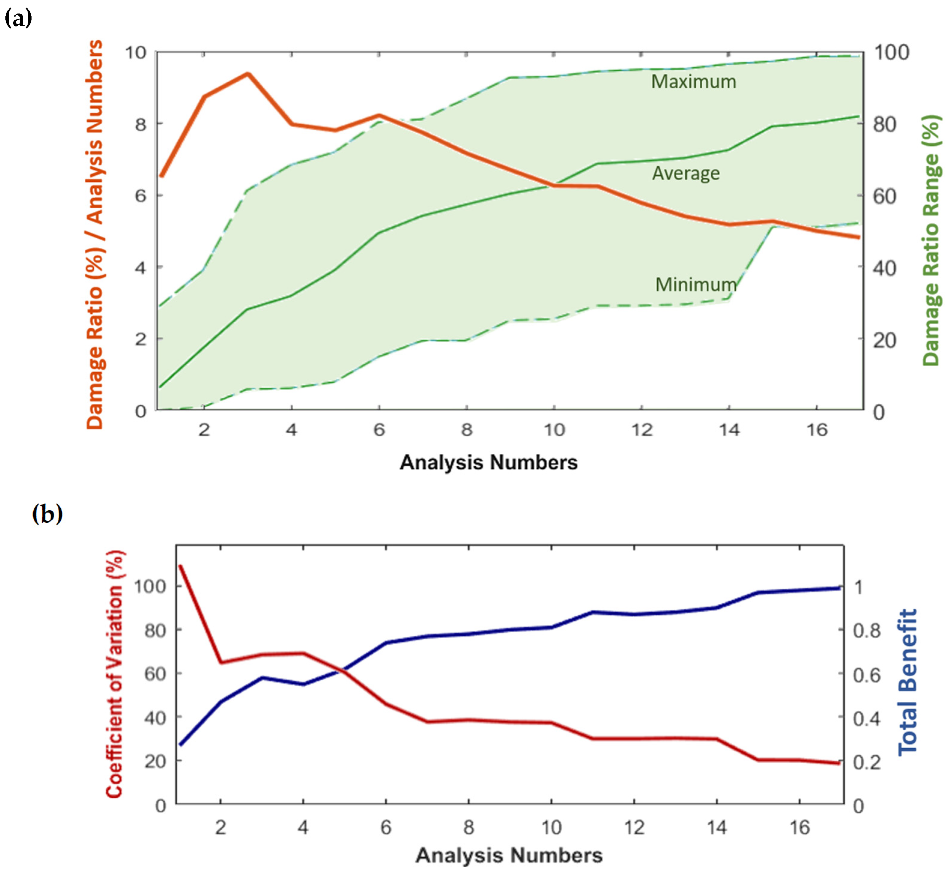
Number of Analysis Sets	Cumulative Probability (%)	Total Benefit	Damage Ratio (%)	Coefficient of Variation (%)
1 (Max Prob.)	24.0	0.27	6.5	109.6
3	48.5	0.58	28.1	68.4
5	62.9	0.62	39.0	60.4
7	70.3	0.77	54.1	37.7
9 (Pr-9U)	75.3	0.80	60.3	37.7
11	78.0	0.88	68.6	30.0
13	79.8	0.88	70.2	30.3
15	81.4	0.97	79.0	20.3
17	82.6	0.99	81.8	18.7

), where only odd M is presented in the table for clarity. The efficiency increases if a higher damage ratio with fewer analyses is achieved. First, the maximum, average, and minimum damage ratio values are plotted, as in Figure 10a, to present the damage ratio range of each analysis sets and the damage ratio gain per analysis set. When M is assumed to be 3, the average value of the damage ratio is 28.1%. By dividing this value by 3, we obtain 9.4%. This implies that only three sets are required for the analyses. In this case, the total benefit is 0.58, and the corresponding coefficient of variation is 68.4%. These values would be sufficient for an estimation in a preliminary design.

We also plotted the total benefit value and coefficient of variation against M, as per Figure 10b. If a higher benefit value (for example, 0.8) is required, then an M value of 9 is recommended, because the threshold value of 0.8, a damage ratio of 60.3%, and a coefficient of variation of 37.7% are attained. Another viewpoint of the representativeness is the correlation between the cumulative probability and damage ratio, which is plotted as a blue line in Figure 11 by using the data presented in Table 9. M is also marked on the line. We can expect that this line will end at (100%, 100%) when all sea states have been evaluated. That is, the cumulative probability is 100%, and the cumulative damage becomes D_natural, thus resulting in a 100% damage ratio. The total benefit can be seen as the slope of the line from the origin to a dot at a specific M value. Thus, we draw an ideal line in black color, which presents perfect representativeness of selected sea states; that is, the total benefit is 1. Moreover, the blue line is always below the ideal condition, although the selection method attempted to maximize it. The blue line approaches the black line when M increases, which means that the cumulative damage has been fully represented. Then, D_natural can be directly computed as the current (M = 17) cumulative damage divided by the current cumulative probability.

5. Conclusions

This study used the jacket X-type substructure for time-domain dynamic analysis in the waters of the Fuhai area in Taiwan to evaluate the cumulative fatigue damage over a design life of 20 years. This study used SACS to set the wave height and period information of the wave environment, analyze the dynamic response of the structures, select the brace with the largest damage caused to the joints, and consider three structural response signals (FA, IPB, and OPB) to yield stress concentration. We found the hotspots at which the damage to the joints was the highest and converted the stress signals obtained from correlated Fourier transform to power spectra. The total energy was analyzed using the Dirlik method for conducting fatigue analysis by applying S–N curves.

This study explored whether the natural damage can be approximated through a smaller number of environmental combinations, the damages under many sea states combined with the damages under 120 sea states can be compared in terms of their respective probabilities, and the representative environment can be explored. Various combinational strategies were used in this study; the neighborhood around the most probable sea states and the probability type based on the occurrence probability were selected. Elimination of sea states with lower wave heights has the benefit of yielding higher representative damage ratios. Through evaluating six metocean categories, it is concluded that selecting sea states according to probability rank while filtering out low wave conditions can effectively represent the cumulative damage of a structure. This method greatly reduces the number of analysis sets required, and only a few sea states represent the damage ratio of 28.1% and the coefficient of variation of 68.4%. The proposed selection procedure applied to more sea states in sequence and less than one-sixth sea states fully covers the representativeness.

References

- Renewables Energy Policy Network for the 21st Century. Renewables 2020 Global Status Report; REN21: Paris, France, 2020; Available online: https://www.ren21.net/gsr-2020/ (accessed on 22 August 2020).
- Global Wind Power: 2017 Market and Outlook to 2022. In Global Wind Energy Council; Power & Energy Solutions Wind, England and Wales. 2017. Available online: http://cdn.pes.eu.com/v/20160826/wp-content/uploads/2018/06/PES-W-2-18-GWEC-PES-Essential-1.pdf. (accessed on 29 February 2020).
- Ciang, C.C.; Lee, J.R.; Bang, H.J. Structural health monitoring for a wind turbine system: A review of damage detection methods. Meas. Sci. Technol. 2008, 19, 122001. [Google Scholar] [CrossRef]
- Dong, W.; Moan, T.; Gao, Z.J.E.S. Long-term fatigue analysis of multi-planar tubular joints for jacket-type offshore wind turbine in time domain. Eng. Struct. 2011, 33, 2002–2014. [Google Scholar] [CrossRef]
- Yeter, B.; Garbatov, Y.; Guedes Soares, C. Fatigue damage assessment of fixed offshore wind turbine tripod support structures. Eng. Struct. 2015, 101, 518–528. [Google Scholar] [CrossRef]
- Kim, H.J.; Jang, B.S.; Park, C.K.; Bae, Y.H. Fatigue analysis of floating wind turbine support structure applying modified stress transfer function by artificial neural network. Ocean Eng. 2018, 149, 113–126. [Google Scholar] [CrossRef]
- Zhao, P.Y.; Huang, X.P. An improved spectral analysis method for fatigue damage assessment of details in liquid cargo tanks. China Ocean Eng. 2018, 32, 62–73. [Google Scholar] [CrossRef]
- Yeter, B.; Garbatov, Y. Spectral fatigue assessment of an offshore wind turbine structure under wave and wind loading. In Developments in Maritime Transportation and Exploitation of Sea Resources; Francis & Taylor Group: London, UK, 2013; pp. 425–433. [Google Scholar]
- Van Der Tempel, J. Design of Support Structures for Offshore Wind Turbines. Ph.D. Thesis, Technische Universiteit Delft, Delft, The Netherlands, 2006. [Google Scholar]
- Chian, C.Y.; Zhao, Y.Q.; Lin, T.Y.; Nelson, B.; Huang, H.H. Comparative study of time-domain fatigue assessments for an offshore wind turbine jacket substructure by using conventional grid-based and Monte Carlo sampling methods. Energies 2018, 11, 3112. [Google Scholar] [CrossRef]
- Baarholm, G.S.; Moan, T. Estimation of nonlinear long-term extremes of hull girder loads in ships. Mar. Struct. 2000, 13, 495–516. [Google Scholar] [CrossRef]
- Chen, I.W.; Wong, B.L.; Lin, Y.H.; Chau, S.W.; Huang, H.H. Design and analysis of jacket substructures for offshore wind turbines. Energies 2016, 9, 264. [Google Scholar] [CrossRef]
- Vorpahl, F.; Popko, W.; Kaufer, D. Description of a Basic Model of the "Upwind Reference Jacket” for Code Comparison in the OC4 Project under IEA Wind Annex XXX; Fraunhofer Institute for Wind Energy and Energy System Technology (IWES): Bremerhaven, Germany, 2011. [Google Scholar]
- International Standard IEC 61400-3. Wind Turbines—Part 3: Design Requirements for Offshore Wind Turbines; International Electrotechnical Commission (IEC): London, UK, 2009. [Google Scholar]
- Bai, Y.; Jin, W.L. Marine Structural Design, 2nd ed.; Butterworth-Heinemann: Oxford, UK, 2015. [Google Scholar]
- Det Norske Veritas and Germanischer Lloyd (DNVGL). Fatigue Design of Offshore Steel Structures; DNVGL-RP-C203; DNVGL: Oslo, Norway, 2016. [Google Scholar]
- Dirlik, T. Application of Computers in Fatigue Analysis. Ph.D. Thesis, University of Warwick, Coventry, UK, 1985. [Google Scholar]
- Sherratt, F.; Bishop, N.W.M.; Dirlik, T. Predicting fatigue life from frequency-domain data: Current methods. J. Eng. Integr. Soc. 2005, 18, 12–16. [Google Scholar]
- Miner, M.A. Cumulative Damage in Fatigue. J. Appl. Mech. 1945, 12, 159–164. [Google Scholar]
- Morison, J.R.; O’Brien, M.P.; Johnson, J.W.; Shaaf, S.A. The forces exerted by surface waves on monopiles. J. Pet. Technol. 1950, 2, 149–154. [Google Scholar] [CrossRef]
- Vanem, E. Joint statistical models for significant wave height and wave period in a changing climate. Mar. Struct. 2016, 49, 180–205. [Google Scholar] [CrossRef]
- Jonkman, J.; Butterfield, S.; Musial, W.; Scott, G. Definition of a 5-MW Reference Wind Turbine for Offshore System Development; National Renewable Energy Lab. (NREL): Golden, CO, USA, 2009.