Energy-Saving Train Regulation for Metro Lines Using Distributed Model Predictive Control ^†

Abstract

Due to environmental concerns, the energy-saving train regulation is necessary for urban metro transportation, which can improve the service quality and energy efficiency of metro lines. In contrast to most of the existing research of train regulation based on centralized control, this paper studies the energy-saving train regulation problem by utilizing distributed model predictive control (DMPC), which is motivated by the breakthrough of vehicle-based train control (VBTC) technology and the pressing real-time control demand. Firstly, we establish a distributed control framework for train regulation process assuming each train is self-organized and capable to communicate with its preceding train. Then we propose a DMPC algorithm for solving the energy-saving train regulation problem, where each train determines its control input by minimizing a constrained local cost function mainly composed of schedule deviation, headway deviation, and energy consumption. Finally, simulations on train regulation for the Beijing Yizhuang metro line are carried out to demonstrate the effectiveness of the proposed DMPC algorithm, and the results reveal that the proposed algorithm exhibits significantly improved real-time performance without deteriorating the service quality or energy efficiency compared with the centralized MPC method.

1. Introduction

With the ever-accelerating process of urbanization, transportation infrastructure and traffic management can not meet the growing traffic demand. The traffic congestion is becoming more serious. Urban metro transportation is considered an ideal solution to ease the traffic pressure in large and populous cities due to its huge capacity, safety, and punctuality [1]. However, metro lines are known to be inhrerently unstable since unavoidable disturbances will bring deviations from the scheduled timetable and any deviation will be amplified with time [2,3]. To prevent such instability, online train regulation is very necessary for scheduled timetable recovery by dynamically manipulating the running time and staying time of each train.

As pioneer studies of metro train regulation, Campion et al. [2] and Van Breusegem et al. [3] addressed the state feedback control of metro lines without considering operational constrains. Due to the large-scale, nonlinear, constrained, and stochastic features of metro transportation systems [4,5,6], model predictive control (MPC) [7,8,9] has become a widely used method in solving the train regulation problem. Grube and Cipriano [10] compared MPC strategy with the heuristic rule-based strategy for metro train regulation, showing that MPC strategy has better performance. Lately, Li et al. [11] presented a robust MPC method to address the metro train regulation problem in presence of the uncertain passenger arrival flow and disturbances. Another MPC-based train regulation approach with considering the passengers dynamic effect was proposed [12]. Moaveni and Najafi [13] proposed a robust MPC approach for train regulation in metro loop lines based on a nonlinear uncertain traffic model. Li et al. [14] developed a dynamic optimal control model and presented an MPC approach for metro train regulation, which converted the optimization problem into a set of convex quadratic programming problems so as to satisfy the real-time control requirement.

In addition, Lin and Sheu [15] proposed a novel adaptive optimal control (AOC) approach for metro train regulation with the aid of artificial neural networks, and they [16] also developed an AOC method with considering the influence of traffic modeling errors, which was more robust against disturbance. Li et al. addressed the metro train regulation problem with time-varying passenger arrival flow by using stochastic stability theory and switched system in [17,18], respectively.

Most of the existing literatures on train regulation focus on the objectives of scheduled timetable recovery and headway adherence so that the service quality can be improved. However, the running time and staying time employed by the train regulator will affect the energy consumption of the train operation at the same time. Therefore, it is of great significance to study the energy-saving train regulation problem with the objective of scheduled timetable recovery and headway adherence as well as minimizing the energy consumption at the same time. Till now, the results on energy-saving train regulation are still limited. Lin and Sheu [19] proposed an adaptive optimal control algorithm to solve the energy-saving train regulation problem of metro lines through reinforcement learning. Zhang et al. [20] presented a real-time optimal design for energy-saving train regulation based on centralized MPC (CMPC).

On the other hand, it is worth noting that most of the existing work addressed the train regulation problem based on the centralized control, where the departure time instants of all trains are assumed to be collected nearly simultaneously, and the control of all trains are also assumed to be applied nearly simultaneously. However, this assumption may not be satisfied in real scenarios, and the centralized controller inevitably results in heavy computation and communication cost so as to threaten the real-time control demand. Therefore, it is pressing for us to study the train regulation problem from the perspective of distributed control, which has been a more popular approach to cope with large scale control systems due to its features of low-cost, scalability and robustness [21,22,23]. Basing on distributed MPC (DMPC) [24,25], Li et al. [26] derived a cooperative energy-efficient trajectory planning for multiple high-speed train movement, where all the high-speed trains were modeled as the agents that can communicate with others and each train can regulate the trajectory planning procedure to save energy. To avoid the heavy computation burden caused by centralized railway management, the centralized rescheduling problem was divided into a set of subproblems and solved by the DMPC methods in [27]. To the best of our knowledge, the study on distributed control-based train regulation problem is still scarce. In our previous work [28], we proposed a novel train regulation framework and algorithm based on DMPC. Focusing on the automatic train regulation of large-scale complex urban metro networks, a distributed optimal control method was designed in [29], where the original large-scale optimization problem was decomposed into multiple small-scale optimization subproblems. However, the energy-saving objective was not considered in [28,29].

Therefore, the aim of this paper was to investigate the energy-saving train regulation problem for a single metro line based on DMPC, by assuming each train is self-organized and capable to communicate with other trains. The main contributions of this paper are two-fold. (1) Focusing on the energy-saving train regulation problem, we employ DMPC method instead of centralized control method, so as to avoid the heavy computation and communication cost in [19,20]. (2) In contrast to the previous work on distributed control-based train regulation [28,29], we newly take the energy consumption into account, with the objective of scheduled timetable recovery and headway adherence as well as minimizing the energy consumption at the same time.

The remainder part of this paper is organized as follows. In Section 2, the energy-saving train regulation problem is described with train traffic model and energy consumption model established. In Section 3, a distributed framework for energy-saving train regulation of a metro open line is presented, and then a DMPC algorithm for energy-saving train regulation is proposed. In Section 4, simulations on energy-saving train regulation for the Beijing Yizhuang metro line are provided to verify the effectiveness and advantages of the DMPC algorithm. Section 5 concludes the whole paper.

2. Problem Formulation

In order to be convenient and rigorous in describing the energy-saving train regulation problem, we first give the train traffic model and energy consumption model. In this study, we consider a metro open line which is defined as a sequence of N stations where M trains are operated. These trains are injected at the first station successively and leave the line after station N. To study the train regulation problem more rigorously, we made the following assumptions: (1) the overtaking and crossing operation are prohibited; (2) each train is required to stop at all stations; (3) the staying time of a certain train depends on the arrival passenger flow and increases proportionally with the boarding passenger number of each stop.

2.1. Train Traffic Model of Metro Open Line

We consider a group of orderly trains running on an metro open line. To describe the train regulation problem based on state-space model, we use the number $i-1$ to denote the train ahead of train i. In addition, to describe the train traffic transfer from one station to the next station, we denote k as the station index and $k\in$$\{1,2,\cdots ,N\}$.

Following the commonly used train traffic model [3], let $d_k^i$ denote the departure time instant of train i from station k, $r_k^i$ denote the running time of train i from station k to $k+1$, and $s_k^i$ denote the staying time of train i at station k. As shown in Figure 1, the departure time instant of train i from station $k+1$ is given as

$$d_{k+1}^i=d_k^i+r_k^i+s_{k+1}^i$$

(1)

The running time of train i from station k to $k+1$ is

$$r_k^i=R_k+{u_{r,}}_k^i+{w_{r,}}_k^i$$

(2)

where $R_k$ is the nominal running time from station k to $k+1$, ${u_{r,}}_k^i$ represents the control action to change the running time of train i between stations k and $k+1$, and ${w_{r,}}_k^i$ is the uncertain disturbance related to the running time. The staying time $s_{k+1}^i$ proportionally increases with the number of passengers getting on the train, and it is given as

$$s_{k+1}^i=t_b{\lambda }_{k+1}·\left(d_{k+1}^i-d_{k+1}^{i-1}\right)+S_{k+1}+{u_{s,}}_{k+1}^i+{w_{s,}}_{k+1}^i$$

(3)

where $t_b$ is the average boarding time per passenger, ${\lambda }_k$ is the average passenger arrival rate at station k, $S_k$ is the minimal staying time at station k when no passenger gets on the train, ${u_{s,}}_k^i$ is the control action to change the staying time on train i at station k, and ${w_{s,}}_k^i$ is the uncertain disturbance related to the staying time. Substituting (2) and (3) into (1), the train traffic model for the operation of the metro line is given as follow

$$\begin{array}{cc}\hfill d_{k+1}^i=& c_{1,k+1}·d_k^i-c_{2,k+1}·d_{k+1}^{i-1}+c_{1,k+1}·\left(S_{k+1}+R_k+w_k^i+u_k^i\right)\hfill \end{array}$$

(4)

where

$$\left\{\begin{array}{c}{c}_{1,k+1}=1/\left(1-t_b·{\lambda }_{k+1}\right)\hfill \\ c_{2,k+1}=t_b·{\lambda }_{k+1}/\left(1-t_b·{\lambda }_{k+1}\right)\hfill \\ w_k^i={w_{r,}}_k^i+w_{s,}{}_{k+1}^i\hfill \\ u_k^i={u_{r,}}_k^i+u_{s,}{}_{k+1}^i\hfill \end{array}\right.$$

It is obvious that the departure time instant of train i from station $k+1$ is directly related to not only that of train i from station k but also that of train $i-1$ from station $k+1$. we let $a_{k+1}^i$ denote the actual arrival time instant of train i station $k+1$, which can be defined as:

$$a_{k+1}^i=d_k^i+r_k^i$$

(5)

Let $D_k^i$ denote the scheduled (nominal) departure time instant of train i from station k and $D_k^{i+1}-D_k^i=H$, where H denotes the scheduled headway. Then the scheduled departure time is

$$D_{k+1}^i=D_k^i+S_{k+1}+R_k+t_b·{\lambda }_{k+1}·H$$

(6)

2.2. Modeling Energy Consumption

In this part, the model which represent the energy consumption arising from train regulation will be formulated. For an urban rail train, the energy consumption mainly comes from the auxiliary system and the traction system when the train is traveling from one station to the next [30].

According to [31], the energy consumption are given as

$$E_{k+1}^i=E_{\mathrm{aux},k+1}^i+E_{\mathrm{tr},k+1}^i$$

(7)

where $E_{k+1}^i$ is energy consumption of train i among time interval $[d_i^k,d_{k+1}^i)$; $E_{\mathrm{aux},k+1}^i$ and $E_{\mathrm{tr},k+1}^i$ represent the energy consumption of the auxiliary system and traction system among time interval $[d_i^k,d_{k+1}^i)$, respectively.

2.2.1. Modeling Energy Consumption of Auxiliary System

Considering an urban rail train, the energy consumption generated by the auxiliary system mainly comes from air conditioning, ventilation and lighting facilities, in which the air conditioning accounts for the largest proportion. On the one hand, the energy consumption generated by the air conditioner is affected by the weather and climate conditions, but also depends on the onboard passenger load. Assuming that the energy consumption of air conditioning is linearly proportional to the onboard passenger load, the energy consumption of auxiliary system among time interval $[d_i^k,d_{k+1}^i)$ can be modeled as follows [31]:

$$\begin{array}{cc}\hfill E_{\mathrm{aux},k+1}^i& =P_{\mathrm{aux},k}^i(d_{k+1}^i-d_k^i)=(P_{\mathrm{ac}}{p}_{k+1}^i+P_{\mathrm{lc}})(d_{k+1}^i-d_k^i)\hfill \end{array}$$

(8)

where $P_{\mathrm{aux},k}^i\stackrel{\Delta }{=}{P}_{\mathrm{ac}}{p}_{k+1}^i+P_{\mathrm{lc}}$ represent the auxiliary power generated by the ith train running from the kth station to the $(k+1)$th station. $P_{\mathrm{ac}}$ is the power generated by per passenger in train and $P_{\mathrm{lc}}$ is the power consumption of the auxiliary facilities otherwise.

In (8), $p_{k+1}^i$ is the the number of passengers in train i from station k to station $k+1$, which can be calculated by using the following passenger equation [32]:

$$p_{k+1}^i=p_k^i+{\xi }_k^i(d_k^i-d_k^{i-1})-\sum _{q=1}^{k-1}{\zeta }_{q,k}^i(d_q^i-d_q^{i-1}),$$

(9)

$$p_0^i=0$$

(10)

where ${\xi }_k^i$ is the boarding passenger’s flow rate of train i at station k, ${\zeta }_{q,k}^i$ is the boarding passenger’s flow rate of the $i\mathrm{th}$ train at upstream station q and bounding for station k.

The ${\xi }_k^i$ and ${\zeta }_{q,k}^i$ can be obtained from the OD (Origin-Destination) of passenger flow. The three terms on the right side of (9), in that respective order, are the passengers in the $i\mathrm{th}$ train when arriving at station k, the passengers boarding the $i\mathrm{th}$ train at the $k\mathrm{th}$ station and bound for downstream stations, and the passengers boarding the $i\mathrm{th}$ train on the upstream qth (q from 1 to $k-1$) station and alighting at the $k\mathrm{th}$ station. The nominal onboard passenger load model can be described as follows:

$$p_{k+1}^i=p_k^i+{\overline{\xi }}_k(d_k^i-d_k^{i-1})-\sum _{q=1}^{k-1}{\overline{\zeta }}_k(d_q^i-d_q^{i-1}),p_0^i=0$$

(11)

where ${\overline{\xi }}_k$ and ${\overline{\zeta }}_k$ are the mean boarding passenger flow rates of ${\xi }_k^i$ and ${\zeta }_{q,k}^i$, respectively.

2.2.2. Modeling Energy Consumption of Traction System

The traction energy consumption is related to the coasting point and the onboard passengers when the train runs between stations, and a good coasting point can effectively reduce the energy consumption by the traction system [33]. As stated in [31], the  energy consumed by the traction system is a non-increasing function of run time. Therefore, the traction energy consumption can be changed by changing the running time. Furthermore, the running time can be adjusted by changing the coasting point. Due to the analytical form of the traction energy consumption being not available, a numerical method can be used to get the traction energy consumption [31]. It can be modeled as follows:

$$E_{\mathrm{tr},k+1}^i=(1+{\omega }_p{p}_{k+1}^i)(\frac{{\mu }_{1,k}}{{\mu }_{2,k}-r_k^i}+{\mu }_{3,k})$$

(12)

where ${\omega }_p\stackrel{\Delta }{=}(W_p/W_1)$, $W_p$ is the mean passenger weight, $W_1$ is the tare weight of the train, $p_{k+1}^i$ is the onboard passenger load defined by (9). ${\mu }_{.,k}$ is the coefficient, which can be obtained by nonlinear fitting method [19].

3. Distributed Model Predictive Control for Energy-Saving Train Regulation

As far as we know, most of the existing researches on train regulation are centralized control methods. Using centralized control methods, one needs to assume that the departure time instants of each train are known nearly simultaneously, which is difficult to match the actual situation. A central server is necessary to deal with the regulation problem of all trains. Meanwhile, the information of all trains needs to be transmitted to the central server, which greatly increases the burden of communication and computation.

On the other hand, with the emergence and development of the new generation of train control technology, VBTC technology will become the focus of the next generation train control technology, because it has the characteristics of low cost, modularization, high performance, and reliability. VBTC technology breaks through the centralized control mode based on ground command and realizes the on-board train operation control mode. Therefore, it becomes possible to apply distributed control to addressing the train regulation problem, in order to reduce the communication and computation cost.

Motivated by this, we firstly present a distributed control framework for energy-saving train regulation in metro open lines, and then propose a DMPC algorithm for energy-saving train regulation of metro open lines with operational constraints taken into account.

3.1. Distributed Control Framework

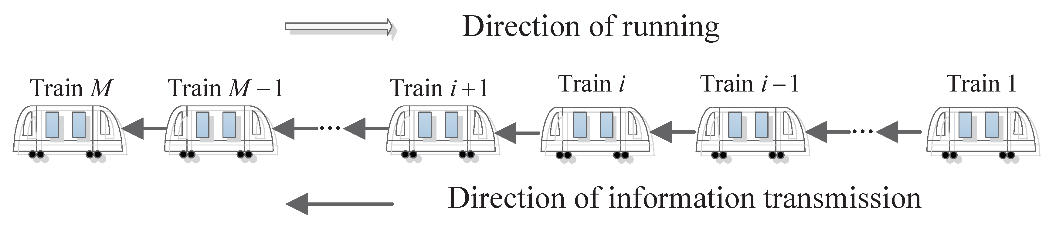
In contrast to the exiting train regulation studies based on centralized control, we assume each train is self-organized and capable to communicate with other trains. We use the predecessor-following topology as shown in Figure 2 to model the communication between trains in the metro open line. More explicitly, train i transmits information to train $i+1$, and it can only receive the information from train $i-1$. Herein, we focus on the design of the control law $u_k^i$ in Equation (4) for each train by using the DMPC method.

3.2. Distributed Model Predictive Control Algorithm

In this subsection, we mainly propose a DMPC algorithm for energy-saving train regulation in metro open lines, where each train determines its control input by optimizing a local constrained cost function involving the information of its own and its predecessor.

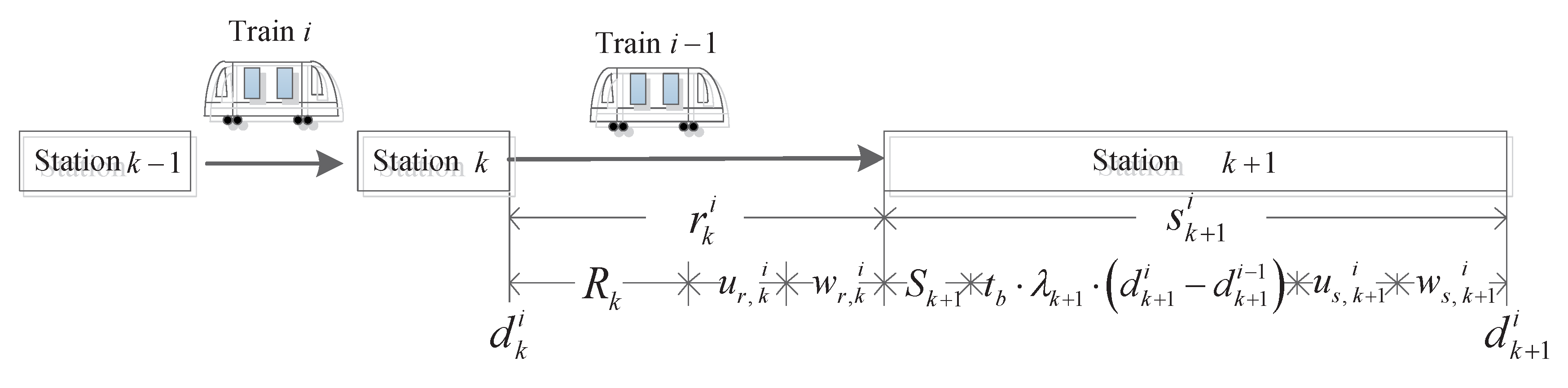
The main objective of energy-saving train regulation is to minimize the schedule deviation, headway deviation, and energy consumption. Then the cost function of each train i at station k is written as

$$\begin{array}{c}\underset{j=1}{\overset{L}{\Sigma }}\hfill \end{array}\left\{\begin{array}{c}{\alpha }_1·{\left(d_{k+j|k}^i-D_{k+j}^i\right)}^2\hfill \\ +{\alpha }_2·{\left(d_{k+j|k}^i-d_{k+j}^{a,i-1}-H\right)}^2\hfill \\ +{\alpha }_3·{\left(E_{k+j|k}^i\right)}^2\hfill \\ +{\alpha }_4·{\left({u_{r,}}_{k+j-1|k}^i\right)}^2\hfill \\ +{\alpha }_5·\left({u_{s,}}_{k+j|k}^i\right)\hfill \end{array}\right\}$$

(13)

where L is the prediction horizon, $d_{k+j|k}^i$ denotes the departure time of train i from station $k+j$ predicted at station k, $d_{k+j}^{a,i-1}$ is the assumed departure time of train $i-1$ from station $k+j$, ${\alpha }_1>0$, ${\alpha }_2\ge 0$, ${\alpha }_3\ge 0$, ${\alpha }_4>0$, and ${\alpha }_5>0$. $E_{k+j|k}^i$ is the energy consumption of train i running from station $k+j-1$ to station $k+j$ predicted at station k, ${u_{r,}}_{k+j-1|k}^i$ is the control action to change the running time of train i between stations $k+j-1$ and $k+j$ predicted at station k, and ${u_{s,}}_{k+j|k}^i$ is the control action to change the staying time on train i at station $k+j$ predicted at station k.

The first term in (13) penalizes schedule deviation which is the departure time deviation of train i from the nominal time schedule among the prediction horizon, and it is used to improve punctuality of the metro line. The second term penalizes the headway deviation between trains i and $i-1$ among the prediction horizon, and it is used to enhance the headway regularity so as to improve the passenger satisfaction. The third term denotes total energy consumption, which is used for the purpose of saving energy. The fourth and fifth terms are related to the magnitudes of the control actions, the minimization of which is used for reducing the control cost in real-world applications.

In a real metro line, several operational constraints with respect to control actions and headways need to be taken into account. The control action of train, which is applied by adjusting the running and staying time, should satisfy

$$\begin{array}{c}{U}_{\mathrm{R},min}\le u_{r,k}^i\le U_{\mathrm{R},max}\hfill \\ U_{\mathrm{S},min}\le u_{s,k}^i\le U_{\mathrm{S},max}\hfill \end{array}$$

where $U_{\mathrm{R},min}$ and $U_{\mathrm{R},max}$ are the lower bound and the upper bound of the running time adjustment from station k to station $k+1$, respectively. $u_{r,k}^i<0$ means that train i needs to accelerate when running from station k to $k+1$. When $u_{r,k}^i=U_{\mathrm{R},min}$, it indicates that train i runs with the maximum speed from station k to station $k+1$. $U_{\mathrm{S},min}$ is the lower bound of staying time adjustment at station k and $U_{\mathrm{S},max}$ is the upper bound of staying time adjustment at station k. In addition, to ensure the train operation safety, headway between trains i and $i-1$ should follow the constraint

$$d_k^i-d_k^{i-1}>H_{min}$$

with $H_{min}$ denoting the minimum headway.

Given the cost function and operational constraints, each train i solves the following local MPC optimization problem

$$\underset{{\left\{\genfrac{}{}{0pt}{}{u_{r,k+j-1|k}^i\hfill }{u_{s,k+j|k}^i\hfill }\right\}}_{j=1}^L}{min}\sum _{j=1}^L\left\{\begin{array}{c}{\alpha }_1·{\left(d_{k+j|k}^i-D_{k+j}^i\right)}^2\hfill \\ +{\alpha }_2·{\left(d_{k+j|k}^i-d_{k+j}^{a,i-1}-H\right)}^2\hfill \\ +{\alpha }_3·{\left(E_{k+j|k}^i\right)}^2\hfill \\ +{\alpha }_4·{\left({u_{r,}}_{k+j-1|k}^i\right)}^2\hfill \\ +{\alpha }_5·{\left({u_{s,}}_{k+j|k}^i\right)}^2\hfill \end{array}\right\}$$

(14)

subject to (15)–(23) to obtain ${\left\{u_{r,k+j-1|k}^{i*},u_{s,k+j|k}^{i*}\right\}}_{j=1}^L$ and ${\left\{d_{k+j|k}^{i*}\right\}}_{j=1}^L$ at station k.

$$\begin{array}{c}\{\begin{array}{}\mathrm{(15)}& d_{k|k}^i=d_k^i\mathrm{(16)}& d_{k+j+1|k}^i=c_{1,k+j}·d_{k+j|k}^i-c_{2,k+j}·d_{k+j+1}^{a,i-1}+c_{1,k+j}·\left(S_{k+j}+R_{k+j-1}+u_{r,k+j-1|k}^i+u_{s,k+j|k}^i\right)\mathrm{(17)}& p_{k+j+1|k}^i=p_{k+j|k}^i+{\xi }_{k+j}^i(d_{k+j}^i-d_{k+j}^{i-1})-{\displaystyle \sum _{q=1}^{k+j-1}}{\zeta }_{q,k+j}^i(d_q^i-d_q^{i-1})\mathrm{(18)}& E_{k+j|k}^i=E_{\mathrm{tr},k+j|k}^i+E_{\mathrm{aux},k+j|k}^i\mathrm{(19)}& E_{\mathrm{tr},k+j+1|k}^i=(1+{\omega }_p{p}_{k+j+1|k}^i)(\frac{{\mu }_{1,k+j}}{{\mu }_{2,k}-r_{k+j}^i}+{\mu }_{3,k+j})\mathrm{(20)}& E_{\mathrm{aux},k+j+1|k}^i=(P_{\mathrm{ac}}{p}_{k+j+1|k}^i+P_{\mathrm{lc}})(d_{k+j+1|k}^i-d_{k+j|k}^i)\mathrm{(21)}& U_{\mathrm{R},min}\le u_{r,k+j-1|k}^i\le U_{\mathrm{R},max}\mathrm{(22)}& U_{\mathrm{S},min}\le u_{s,k+j|k}^i\le U_{\mathrm{S},max}\mathrm{(23)}& d_{k+j|k}^i-d_{k+j}^{a,i-1}>H_{min}\end{array}\end{array}$$

Equation (15) represents the actual time when train i departs from station k. The predicted departure time of train i from station $k+j$ when train i departs from station k can be computed iteratively by Equation (16), which is straightforward from Equation (4). The predicted number of passengers in train i from station $k+j$ to station $k+j+1$ when train i departs from station k can be computed iteratively by Equation (17), which is straightforward from Equation (9). The total energy consumption, auxiliary energy consumption and traction energy consumption in the prediction horizon are described by Equations (18)-(20), the constraints of running time adjustment and staying time adjustment in the prediction horizon are given in Equations (21) and (22), respectively. Inequality (23) represents the headway constrains in the prediction horizon.

Note that in (14), the assumed departure time sequence of train $i-1$, i.e., ${\left\{d_{k+j}^{a,i-1}\right\}}_{j=1}^L$, is obtained as follows. When train $i-1$ is ready to depart from station k at $d_k^{i-1}$, train $i-1$ solves the optimization problem to obtain ${\left\{d_{k+j|k}^{i-1*}\right\}}_{j=1}^L$, and then transmits $d_k^{i-1}$ and ${\left\{d_{k+j|k}^{i-1*}\right\}}_{j=1}^L$ to train i. Then, train i updates the assumed departure time of train $i-1$, i.e., $d_k^{a,i-1}=d_k^{i-1}$ and $d_{k+j}^{a,i-1}=d_{k+j|k}^{i-1*},j=1,2,\cdots ,L$. When train $i-1$ is ready to depart from station $k+1$ at $d_{k+1}^{i-1}$, the whole process repeats and the assumed departure time sequence of train $i-1$ is updated.

Then we present the DMPC algorithm for energy-saving train regulation in a metro open line, which is presented in Algorithm 1 below.

Algorithm 1 DMPC algorithm for energy-saving train regulation

1: When train i is ready to depart from station k at $d_k^i$, it solves the constrained optimization problem (14) to obtain ${\left\{u_{r,k+j-1|k}^{i*},u_{s,k+j|k}^{i*}\right\}}_{j=1}^L$ and ${\left\{d_{k+j|k}^{i*}\right\}}_{j=1}^L$. 2: Train i transmits $d_k^i$ and ${\left\{d_{k+j|k}^{i*}\right\}}_{j=1}^L$ to train $i+1$, and then train $i+1$ updates its assumed departure time sequence of train i, i.e, ${\left\{d_{k+j}^{a,i}\right\}}_{j=0}^L$. 3: Train i adjusts its running time and staying time according to $u_{r,k|k}^{i*},u_{s,k|k}^{i*}$. 4: When train i is ready to depart from station $k+1$ at $d_{k+1}^i$, let $k=k+1$ and go to Step 1.

Remark 1.

In the proposed DMPC algorithm, each train collects the information of its own and its predecessor such that the communication cost is significantly reduced. Moreover, each train solves a local optimization problem of small size, and its computation complexity is independent of the scale of the metro transportation system, which implies that the proposed DMPC algorithm is efficiently solvable and scalable.

Remark 2.

It is still challenging for us to further prove the feasibility and convergence of the proposed DMPC algorithm, which is excluded in this paper. We will focus on the corresponding theoretical analysis in our future work.

4. Simulation Results

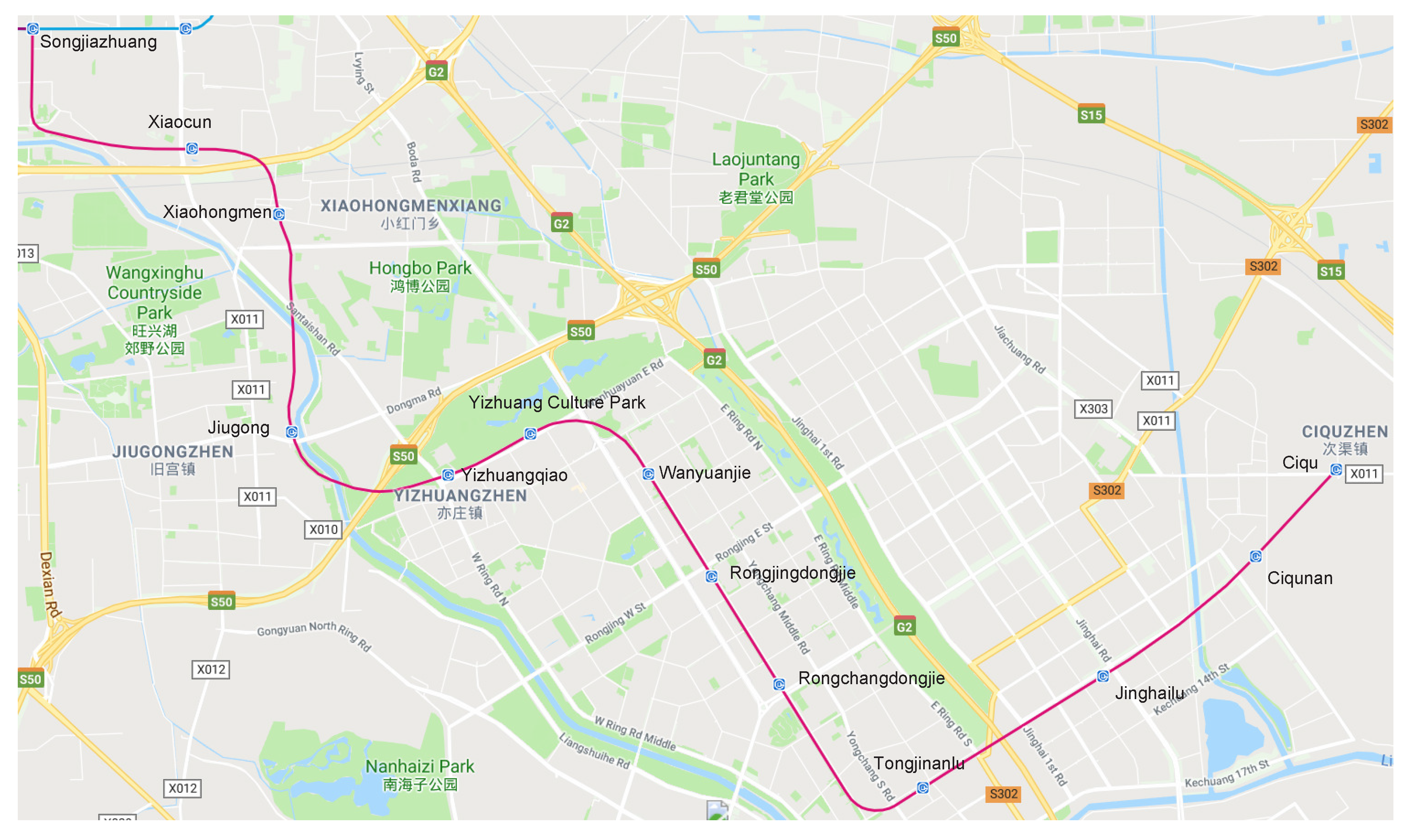
In this section, in order to verify the efficiency of the designed approach for energy-saving train regulation of urban metro line, the proposed DMPC algorithm will be applied to actual Beijing Yizhuang metro line to implement the numerical experiments. Figure 3 shows the map of Beijing Yizhuang metro line, and there are 13 stations and 12 sections on the line. (i.e., N = 13). All computations throughout the following numerical experiments are performed by MATLAB R2016b on a PC (3.30 GHz processor speed and 8-GB RAM) with Microsoft Windows 7 platform, and we use “fmincon” function from the MATLAB optimization tool box to solve the optimization problem (14).

Next, we will describe the experimental environment and related parameters to be set. In the numerical experiment, we only take one direction into account, which is from Songjiazhuang to Ciqu. It is generally true that the passenger flow is very large during the morning and evening peak hours, and the delay propagation can easily be caused by the accumulation of passenger arrival flow. In our simulations, the train regulation is carried out throughout the morning peak hours (form 7:00 a.m. to 8:30 a.m.), where 7:00 a.m is set as 0 second (s). Considering the real operating conditions, the schedule headway H is 270 s, the number of running trains is 20, and the minimum headway is set as 90 s (i.e., $H_{min}=90$)S. We chose the prediction horizon equal to 4 (i.e., $L=4$). The constraints of control values are set as $U_{\mathrm{R},min}=U_{\mathrm{S},min}=-30$ s, and $U_{\mathrm{R},max}=U_{\mathrm{S},max}=35$ s, respectively, indicating that the adjustment values of the staying time and the running time can neither exceed 35 s nor be smaller than −30 s. Due to the fact that the metro train operation is inevitably influenced by uncertain disturbances, we set ${w_{s,}}_k^i$ and ${w_{r,}}_k^i$ to be stochastic ranging from 0 to 15. In our simulation, we assume $P_{\mathrm{ac}}=110\mathrm{W}/\mathrm{passenger}$ and $P_{\mathrm{lc}}=50\mathrm{kW}/\mathrm{train}$.

In order to verify the efficiency of the DMPC strategy, we firstly make a comparison among the performance of the proposed DMPC strategy, the CMPC strategy proposed in [20] and zero control strategy (without train regulation). Next, we show the effects of different values of weights on schedule deviation, headway deviation, and energy consumption.

4.1. Performance Comparison with Other Strategies

In order to validate the effectiveness and merit of the proposed DMPC strategy for energy-saving train regulation, we analyzed the performance of three strategies: the proposed DMPC strategy (i.e., Case 2), the CMPC strategy (i.e., Case 3), and the zero control strategy (i.e., Case 1, in which the ${u_{r,}}_k^i=0$ and ${u_{s,}}_k^i=0$). Both in the DMPC and CMPC algorithms, the weights with respect to schedule deviation, headway deviation, running time control action, and staying time control action are set fixed, which are ${\alpha }_1=10$, ${\alpha }_2=0.01,{\alpha }_4={\alpha }_5=0.1$), and the weight of energy consumption is set as ${\alpha }_3=1$. 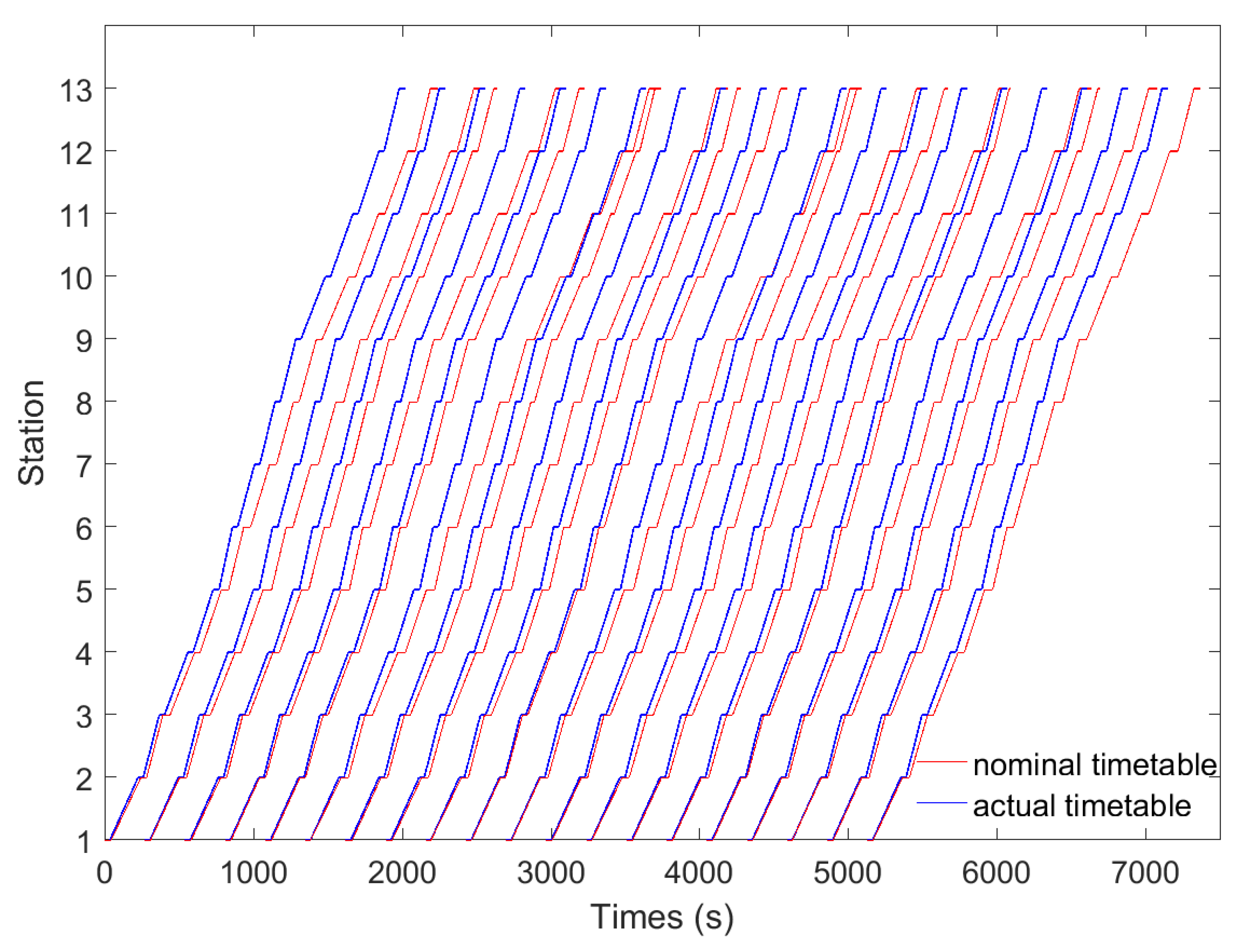The actual timetable under Case 1, Case 2 and Case 3 in contrast to the nominal timetable are respectively shown in Figure 4, Figure 5 and Figure 6.

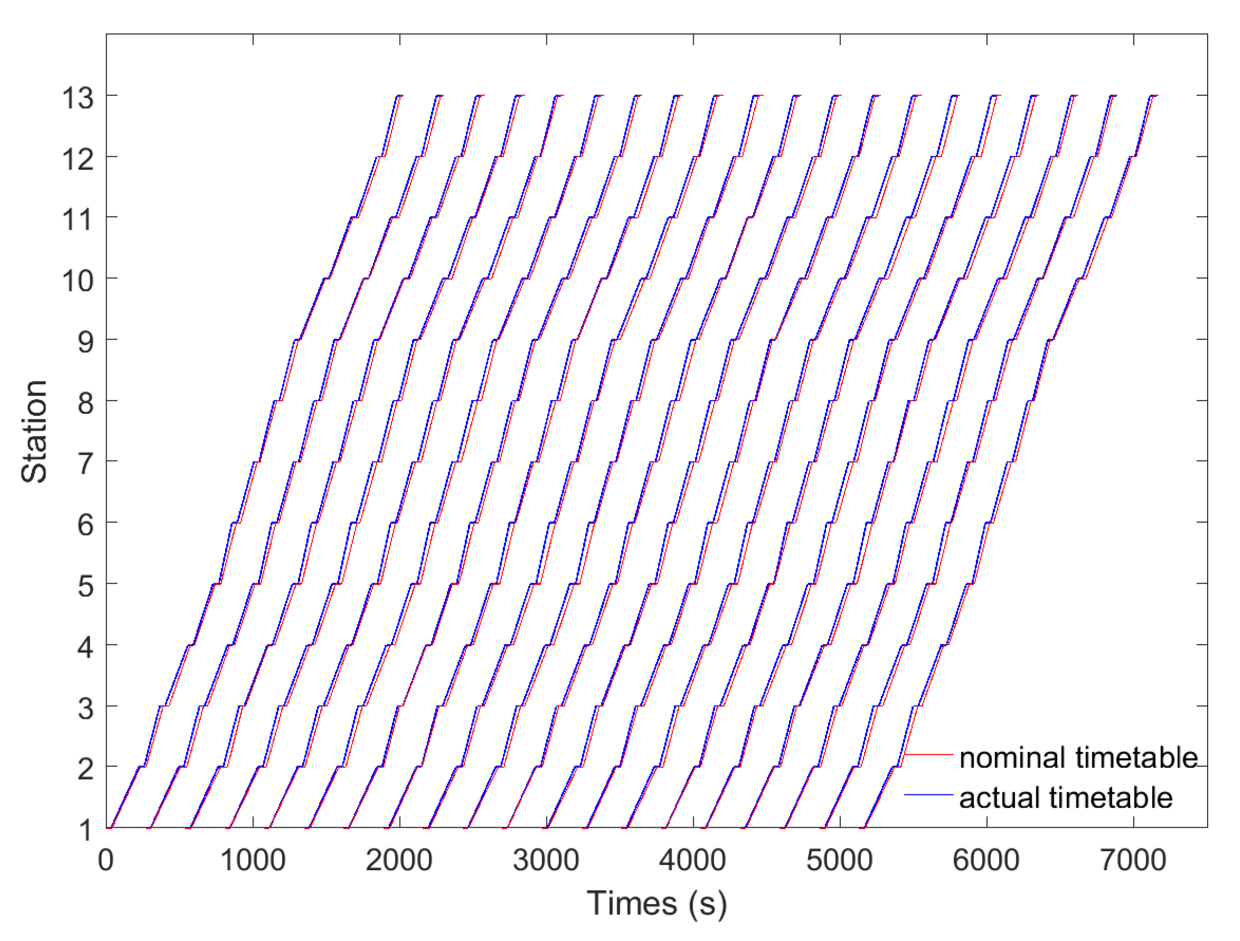
4.1.1. Case 1 (Zero Control Strategy)

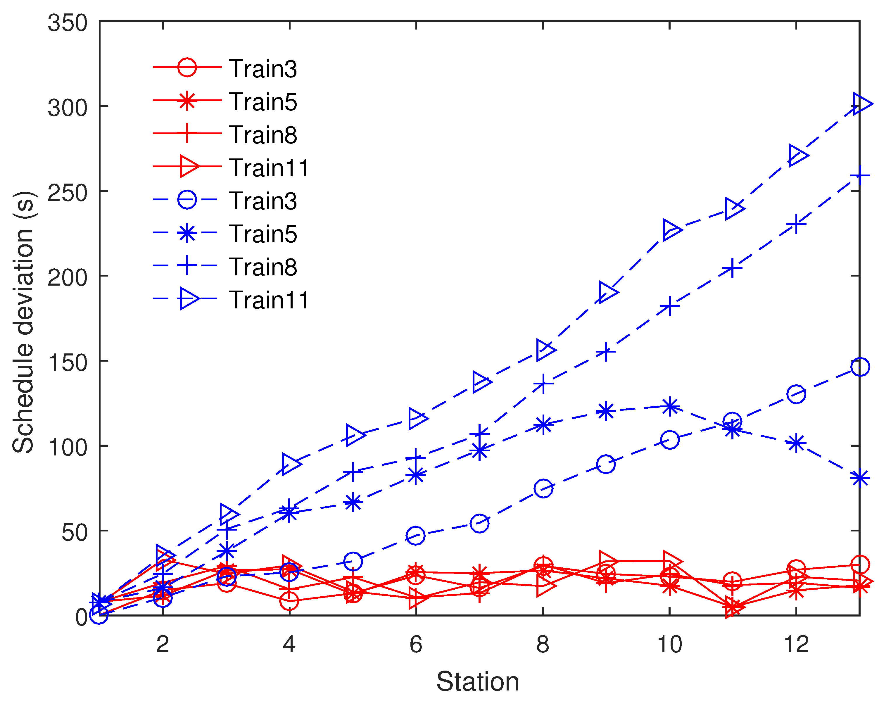
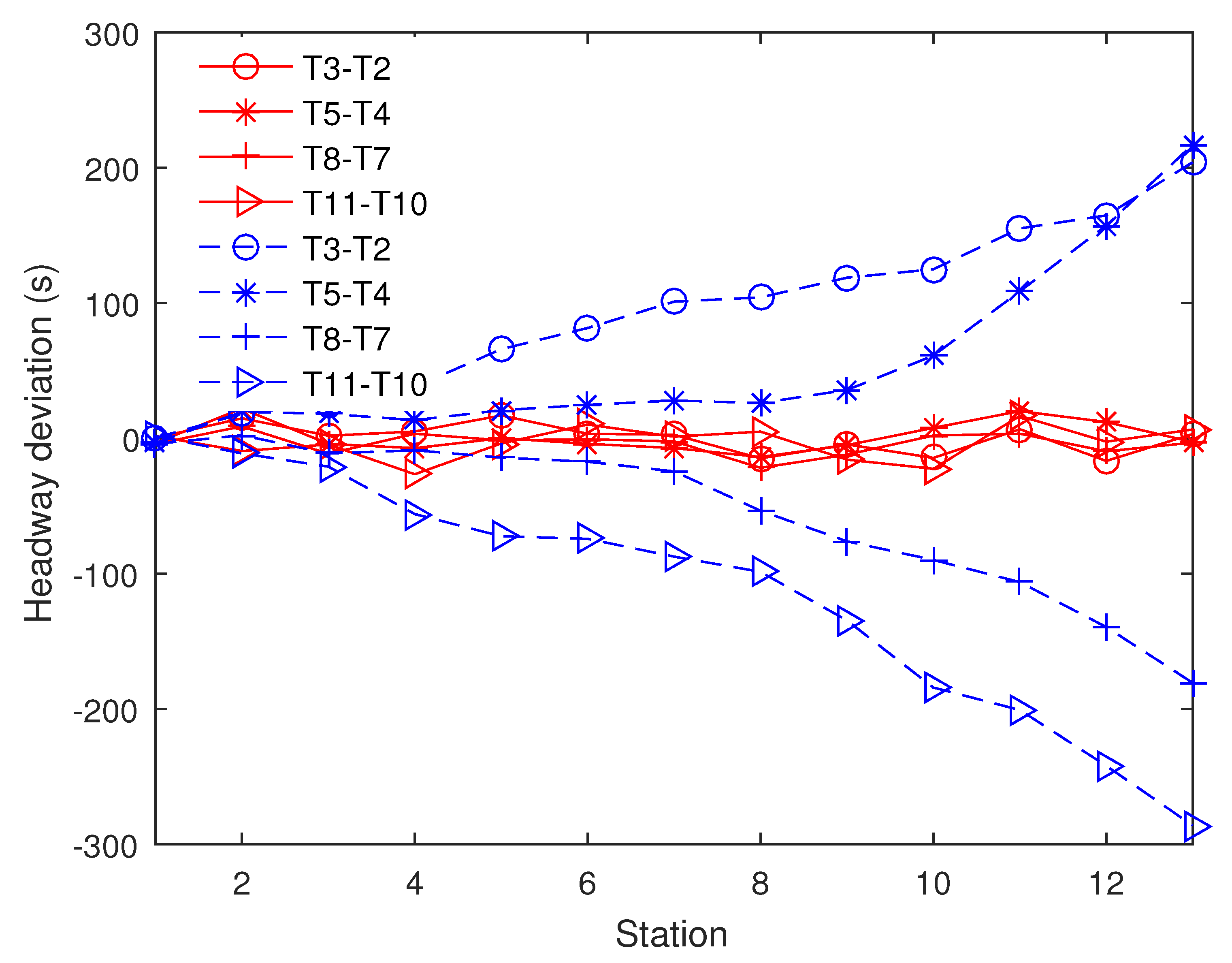
In this case, we only consider the basic constraint conditions, which include the safety constraint and staying time constraint and do not adopt any adjustment method. Then, we got the schedule deviation and the headway deviation, which are respectively displayed in Figure 7 (dashed blue lines) and Figure 8 (dashed blue lines), for clarity.

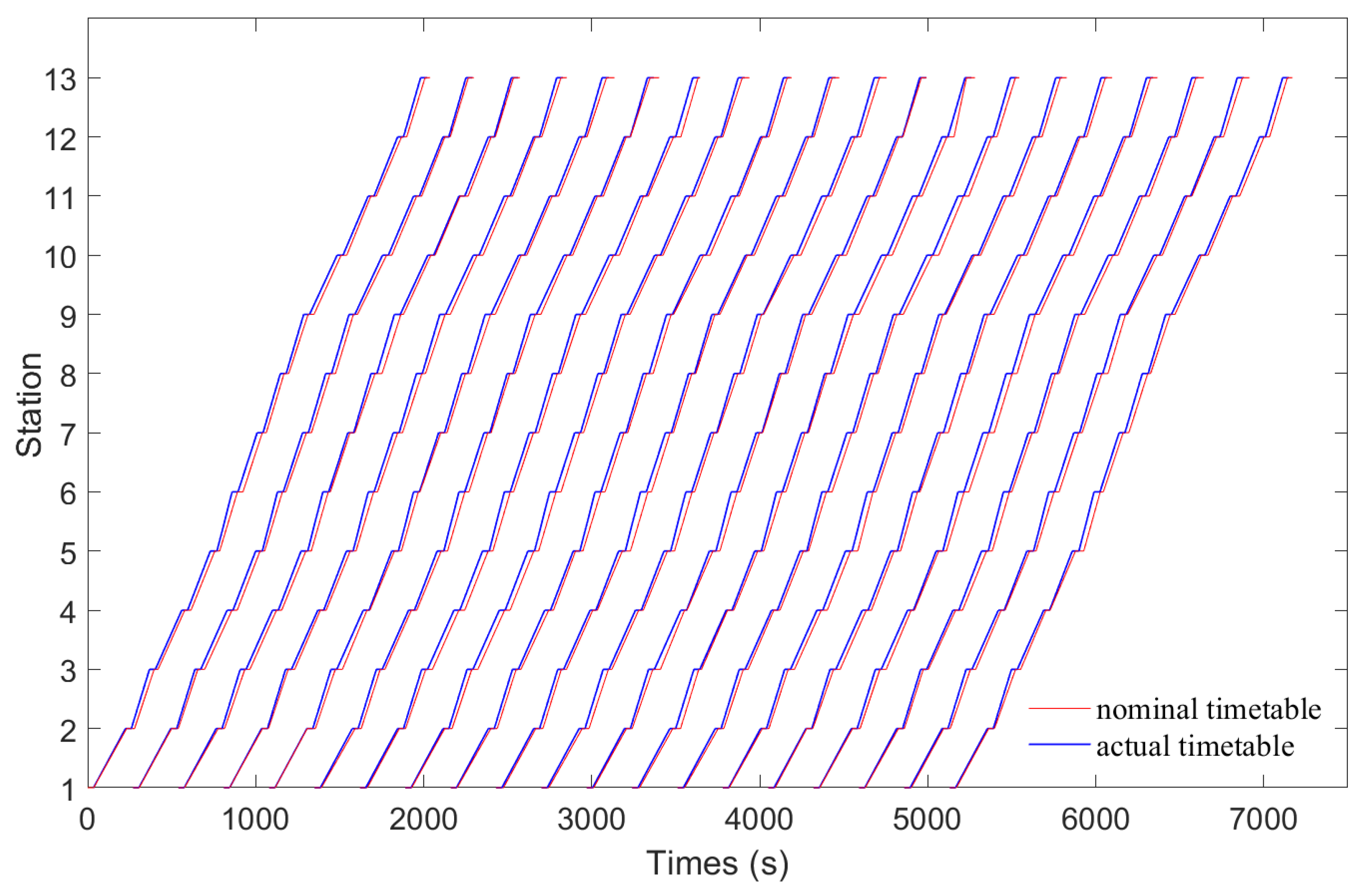
4.1.2. Case 2 (DMPC Strategy)

In this case, the proposed DMPC algorithm is applied to simulate the operation of the metro line. Then, we obtain the schedule deviation and the headway deviation, which are shown in Figure 7 (solid red lines) and Figure 8 (solid red lines) respectively.

4.1.3. Case 3 (CMPC Strategy)

In this case, the CMPC algorithm proposed in [20] is applied to simulate the operations of metro line.

In order to verify the effectiveness of the proposed DMPC algorithm, we firstly make a comparison between DMPC strategy (Case 2) and the zero control strategy (Case 1). From Figure 4, we can easily observe that in Case 1, the deviations from the nominal timetable caused by uncertain disturbances are amplified with time. While in Case 2, as shown by Figure 5, the deviations from the nominal timetable are regulated within a much smaller range. To make a quantized comparison, the trajectories of schedule deviation of certain trains along stations under Case 1 and Case 2 are plotted in Figure 7, and so is the headway deviation as shown in Figure 8. In Figure 7, the schedule deviations under Case 1 are amplified with time and exceed 300 s, while under in Case 2, the schedule deviations are regulated below 35 s. In Figure 8, the headway deviations under Case 1 are also amplified with time and exceed 200 s, while the headway deviations under Case 2 are regulated within (−30 s, 30 s). Till now, we conclude that the schedule deviations and headway deviations in Case 2 are all controlled in a much smaller range compared with Case 1, indicating that the DMPC method significantly improves the regulation performance when compared with the case without control.

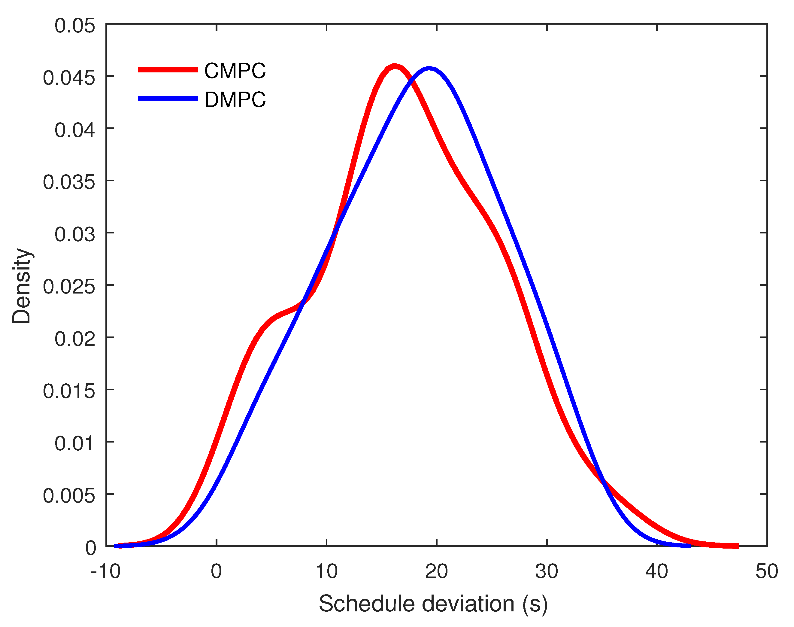
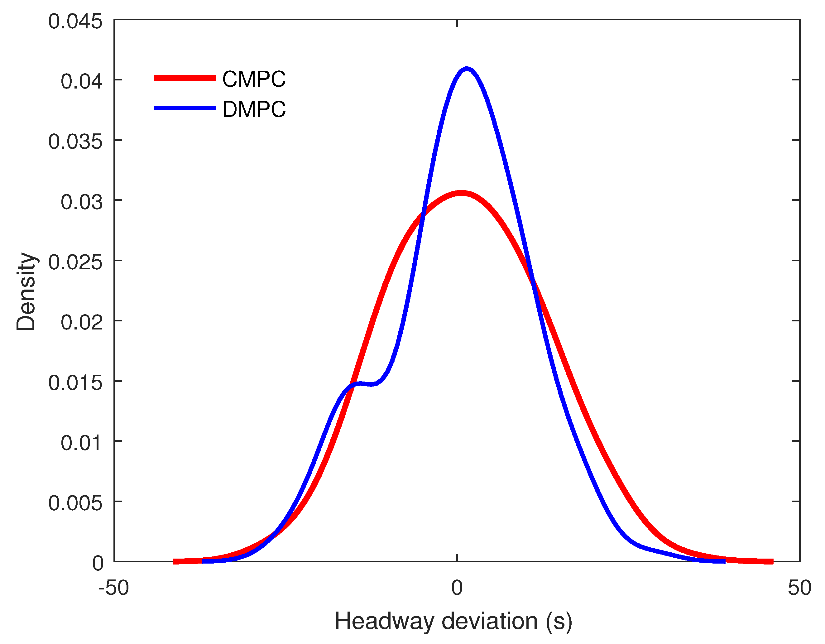
Moreover, we compare the regulation performance of Case 2 with that of Case 3 by giving the probability density distribution of both schedule deviation and headway deviation which are shown in Figure 9 and Figure 10. From Figure 9, we can easily obtain that the mean, the maximum, and distribution shape of schedule deviation are all almost the same under Case 2 and Case 3, and so are those of headway deviation as shown in Figure 10. Then, we can conclude that the DMPC method exhibits comparable regulation performance as CMPC method.

To make a more comprehensive comparison, we calculate the statistical characteristics of schedule deviation, headway deviation, energy consumption and computational time under all the three cases, which are shown in

Table 1. Performance statistics of train regulation.

	Schedule		Headway		Energy	CT
	Deviation		Deviation		Consumption
	(s)		(s)		(kwh)	(s)
	SD	Mean	SD	Mean
NC	77.0	104.2	89.7	60.9	4533	–
CMPC	7.8	16.5	10.2	8.1	3999	5.2
DMPC	7.6	16.6	9.6	7.5	4362	0.02

SD—standard deviation, NC—without control, CT—computational time.

. Note that the energy consumption refers to the energy consumed by a train running from the first station to the terminal station. From Table 1, we can obtain that under case 2, the means of schedule and headway deviations respectively decrease by average of 90.0% and 89.6% compared with Case 1, and the energy consumption decreases by an average of 3.7% compared with Case 1. It can be observed that the performance of the DMPC is not as good as that of the CMPC, but it is close to the CMPC. The computational time of the proposed DMPC method and the CMPC is 0.02s and 5.2s, respectively. Remarkably, the computational time of the proposed DMPC method is far less than that of the CMPC method. This shows that the distributed control method can remarkably improve the real-time performance without sacrificing the service quality or energy efficiency.

4.2. Effects of Different Weights on Performance

In this subsection, in order to balance the punctuality, regularity, and energy efficiency, the sensitivity analysis is carried out for weights ${\alpha }_1$, and ${\alpha }_3$ in cost function (7). By only changing one of these weights, the effects of it on schedule deviation, headway deviation, and energy consumption of the train are analyzed.

Firstly, we analyze the effects of ${\alpha }_1$ on the regulation performance. In this simulation, we let ${\alpha }_2$ = 0.01, ${\alpha }_4$ = ${\alpha }_5$ = 0.1, ${\alpha }_3$ = 1. Four cases with different values of ${\alpha }_1$ are given, and the corresponding simulation results are shown in

Table 2. The effects of ${\alpha }_1$ on the regulation performance.

${\mathit{\alpha }}_1$	Schedule Deviation (s)		Headway Deviation (s)		Energy Consumption (kwh)
	SD	Mean	SD	Mean
1	7.90	17.73	9.55	7.44	4362
2	7.68	16.95	9.59	7.45	4361
5	7.64	16.68	9.62	7.48	4362
10	7.63	16.58	9.64	7.49	4362

. With the increase of ${\alpha }_1$, both the standard deviation and the mean of the schedule deviation are decreasing, while the standard deviation and the mean of the headway deviation are increasing. At the same time, we also notice that the adjustment of ${\alpha }_1$ has little effect on the change of energy consumption.

Then, we analyze the influence of ${\alpha }_3$ on the regulation performance. In this case, we let ${\alpha }_1$ = 10, ${\alpha }_2$ = 0.01, ${\alpha }_4$ = ${\alpha }_5$ = 0.1. The simulation results are shown in

Table 3. The effects of ${\alpha }_3$ on the regulation performance.

${\mathit{\alpha }}_3$	Schedule Deviation (s)		Headway Deviation (s)		Energy Consumption (kwh)
	SD	Mean	SD	Mean
1	7.64	16.61	9.64	8.14	4362
2	7.63	16.59	9.63	8.14	4323
5	7.64	16.63	9.63	8.15	4276
10	7.67	16.71	9.62	8.15	4248

. With the increase of ${\alpha }_3$, the energy consumption is obviously reduced, but punctuality and headway regularity performance are slightly worse. That means, if we enlarge ${\alpha }_3$, the energy consumption can be reduced at the expense of deteriorating punctuality and headway regularity.

Thirdly, the effects of ${\alpha }_3$ on the performance of energy consumption and control action is analyzed. We let ${\alpha }_1$ = 10, ${\alpha }_2$ = 0.01, ${\alpha }_4$ = ${\alpha }_5$ = 0.1. The simulation results are given in

Table 4. The effects of ${\alpha }_3$ on the energy consumption and control action.

${\mathit{\alpha }}_3$	Energy Consumption (kwh)	${\mathit{u}}_{\mathit{r}}\_\mathbf{mean}$ (s)	${\mathit{u}}_{\mathit{s}}\_\mathbf{mean}$ (s)
0	4407	−7.4	−6.8
1	4362	−2.7	−11.1
5	4276	4.6	−17.8

. We use $u_r\_\mathrm{mean}$ to indicate the mean of running time control action, and $u_s\_\mathrm{mean}$ to indicate the mean of staying time control action. With the increase of ${\alpha }_3$, the energy consumption is decreasing, $u_r\_\mathrm{mean}$ is increasing, and $u_s\_\mathrm{mean}$ is decreasing. This indicates that increasing running time and reducing staying time can reduce energy consumption.

Lastly, we define the total schedule deviation (TSD) for train i at all stations as $({\displaystyle \sum _k}(d_k^i-D_k^i)(d_k^i-D_k^i){)}^{\frac{1}{2}}$ and the total headway deviation (THD) as $({\displaystyle \sum _k}(d_k^i-d_k^{i-1}-H)(d_k^i-d_k^{i-1}-H){)}^{\frac{1}{2}}$. We let ${\alpha }_2$ = 0.01, ${\alpha }_4$ = ${\alpha }_5$ = 0.1. We give the analysis about the effects of ${\alpha }_1$ and ${\alpha }_3$ on the TSD and THD. The simulation results are given in

Table 5. Total schedule deviation for trains (TSD).

${\mathit{\alpha }}_1$	1	2	5	10	10	10
${\mathit{\alpha }}_3$	1	1	1	1	2	5
T1	68.2	66.7	66.2	65.5	65.5	65.6
T2	78.4	76.7	76.1	75.2	75.3	75.6
T3	61.2	59.7	59.2	58.5	58.5	58.7
T4	74.0	72.6	72.1	71.3	71.4	71.8
T5	66.7	65.1	64.6	63.9	63.9	63.9
T6	78.1	76.1	75.5	74.6	74.6	74.8
T7	75.3	73.3	72.8	72.0	72.0	72.0
T8	70.6	68.5	68.0	67.2	67.2	67.4
T9	64.4	61.9	61.5	60.8	60.8	60.9
T10	60.9	59.3	58.8	58.1	58.1	58.2
T11	76.5	73.8	73.2	72.4	72.4	72.6
T12	74.5	71.8	71.2	70.3	70.4	70.7
T13	73.2	69.5	69.0	68.2	68.2	68.3
T14	72.8	69.4	68.9	68.2	68.2	68.2
T15	79.0	75.1	74.5	73.6	73.6	73.8
T16	57.8	55.2	54.8	54.2	54.2	54.3
T17	63.4	59.3	58.9	58.2	58.2	58.3
T18	65.4	60.4	59.9	59.2	59.2	59.3
T19	62.1	56.3	55.9	55.3	55.3	55.3
T20	70.6	63.8	63.3	62.6	62.6	62.7

and

Table 6. Total headway deviations for trains (THD).

${\mathit{\alpha }}_1$	1	2	5	10	10	10
${\mathit{\alpha }}_3$	1	1	1	1	2	5
D2-D1	31.4	31.7	31.7	31.9	31.8	31.7
D3-D2	32.0	31.9	31.9	31.9	31.9	31.9
D4-D3	29.6	29.9	30.0	30.2	30.1	29.9
D5-D4	41.5	42.2	42.5	42.9	42.9	42.7
D6-D5	39.6	39.5	39.6	39.7	39.7	39.7
D7-D6	33.9	34.4	34.5	34.7	34.7	34.6
D8-D7	37.9	38.5	38.7	39.1	39.1	39.0
D9-D8	30.3	30.7	30.9	31.3	31.2	31.1
D10-D9	36.6	37.1	37.2	37.3	37.3	37.3
D11-D10	38.7	38.5	38.5	38.5	38.5	38.5
D12-D11	34.9	35.0	35.1	35.1	35.1	35.1
D13-D12	41.2	40.6	40.5	40.4	40.4	40.6
D14-D13	33.3	33.7	33.7	33.8	33.8	33.8
D15-D14	35.9	35.7	35.6	35.6	35.6	35.8
D16-D15	44.1	44.0	43.9	43.7	43.7	43.8
D17-D16	18.9	18.5	18.6	18.7	18.7	18.7
D18-D17	25.9	26.0	26.0	26.1	26.1	26.1
D19-D18	28.1	28.5	28.6	28.9	28.8	28.8
D20-D19	28.7	28.9	29.1	29.3	29.3	29.2

. From Table 5, we can observe that with the increase of weight ${\alpha }_1$ and unchanged weight ${\alpha }_3$, the TSD for all the trains are reduced, i.e., the punctuality is improved with the increase of weight ${\alpha }_1$. With the increase of weight ${\alpha }_3$ and the unchanged weight ${\alpha }_1$, the TSD for all the trains are increased, i.e., the punctuality is deteriorated with the increase of weight ${\alpha }_3$. From Table 6, we can observe that with the increase of weight ${\alpha }_1$ and unchanged weight ${\alpha }_3$, the THD for all the trains are increased, i.e., the regularity is deteriorated with the increase of the weight ${\alpha }_1$. With the increase of weight ${\alpha }_3$ and unchanged weight ${\alpha }_1$, the THD for all the trains are increased, i.e., the regularity is deteriorated with the increase of weight ${\alpha }_3$.

Through the above analysis, we can achieve the trade-off between the performance of the punctuality, regularity, and the energy consumption by selecting appropriate weights.

5. Conclusions

This paper has studied the energy-saving train regulation problem in urban metro transportation by using DMPC control. A distributed control framework for train regulation in metro lines has been proposed, based on which, a novel DMPC algorithm for energy-saving train regulation has been proposed. In the DMPC algorithm, each train determines its control input by optimizing a local cost function subject to operational constraints. To validate the proposed DMPC algorithm, we have made several numerical experiments based on Beijing Yizhuang metro line. The simulation results have shown that the proposed algorithm is effective, and its real-time performance is remarkably improved compared with the routine CMPC. The main contributions of this paper are summarized as follows. Firstly, the DMPC method is used to solve the energy-saving train regulation problem, and the predecessor-following topology is adopted, which requires a very low communication cost. Secondly, from the experimental results, the computational cost of the algorithm is greatly reduced without sacrificing the regulation and energy-saving performance. Open research issues to explore may include proving the convergence of the proposed DMPC algorithm and robust DMPC for train regulation under more complex communication topologies.

References

1. Gonzalez-Gil, A.; Palacin, R.; Batty, P.; Powell, J.P. A systems approach to reduce urban rail energy consumption. Energy Convers. Manag. 2014, 80, 509–524. [Google Scholar] [CrossRef] [Green Version]
2. Campion, G.; Vanbreusegem, V.; Pinson, P.; Bastin, G. Traffic regulation of an underground railway transportation system by state feedback. Optim. Control Appl. Methods 1985, 6, 385–402. [Google Scholar] [CrossRef]
3. Vanbreusegem, V.; Campion, G.; Bastin, G. Traffic modeling and state feedback control for metro lines. IEEE Trans. Autom. Control 1991, 36, 770–784. [Google Scholar] [CrossRef] [Green Version]
4. Chang, S.C.; Chung, Y.C. From timetabling to train regulation-a new train operation model. Inform. Softw. Technol. 2005, 47, 575–585. [Google Scholar] [CrossRef]
5. Fernandez, A.; Cucala, A.P.; Vitoriano, B.; de Cuadra, F. Predictive traffic regulation for metro loop lines based on quadratic programming. Proc. Inst. Mech. Eng. F J. Rail Rapid Trans. 2006, 220, 79–89. [Google Scholar] [CrossRef]
6. Hao, S.; Song, R.; He, S.; Lan, Z. Train Regulation Combined with Passenger Control Model Based on Approximate Dynamic Programming. Symmetry 2019, 11, 303. [Google Scholar] [CrossRef] [Green Version]
7. Garcia, C.E.; Prett, D.M.; Morari, M. Model predictive control: Theory and practice-a survey. Automatica 1989, 25, 335–348. [Google Scholar] [CrossRef]
8. Lee, J.H. Model predictive control: Review of the three decades of development. Int. J. Contr. Autom. Syst. 2011, 9, 415. [Google Scholar] [CrossRef]
9. Mayne, D.Q. Model predictive control: Recent developments and future promise. Automatica 2014, 50, 2967–2986. [Google Scholar] [CrossRef]
10. Grube, P.; Cipriano, A. Comparison of simple and model predictive control strategies for the holding problem in a metro train system. IET Intell. Transp. Syst. 2010, 4, 161–175. [Google Scholar] [CrossRef]
11. Li, S.; De Schutter, B.; Yang, L.; Gao, Z. Robust Model Predictive Control for Train Regulation in Underground Railway Transportation. IEEE Trans. Control Syst. Technol. 2016, 24, 1075–1083. [Google Scholar] [CrossRef]
12. Moaveni, B.; Karimi, M. Subway traffic regulation using model based predictive control by considering the passengers dynamic effect. Arab. J. Sci. Eng. 2017, 42, 3021–3031. [Google Scholar] [CrossRef]
13. Moaveni, B.; Najafi, S. Metro Traffic Modeling and Regulation in Loop Lines Using a Robust Model Predictive Controller to Improve Passenger Satisfaction. IEEE Trans. Control Syst. Technol. 2018, 26, 1541–1551. [Google Scholar] [CrossRef]
14. Li, S.; Yang, L.; Gao, Z. Efficient Real-Time Control Design for Automatic Train Regulation of Metro Loop Lines. IEEE Trans. Intell. Transp. Syst. 2019, 20, 485–496. [Google Scholar] [CrossRef]
15. Lin, W.S.; Sheu, J.W. Metro Traffic Regulation by Adaptive Optimal Control. IEEE Trans. Intell. Transp. Syst. 2011, 12, 1064–1073. [Google Scholar] [CrossRef]
16. Sheu, J.W.; Lin, W.S. Adaptive Optimal Control for Designing Automatic Train Regulation for Metro Line. IEEE Trans. Control Syst. Technol. 2012, 20, 1319–1327. [Google Scholar] [CrossRef]
17. Li, S.K.; Yang, L.X.; Gao, Z.Y.; Li, K.P. Robust train regulation for metro lines with stochastic passenger arrival flow. Inf. Sci. 2016, 373, 287–307. [Google Scholar] [CrossRef]
18. Li, S.K.; Yang, L.X.; Gao, Z.Y. Optimal switched control design for automatic train regulation of metro lines with time-varying passengers arrival flow. Transp. Res. Part C Emerg. Technol. 2018, 86, 425–440. [Google Scholar] [CrossRef]
19. Lin, W.S.; Sheu, J.W. Optimization of Train Regulation and Energy Usage of Metro Lines Using an Adaptive-Optimal-Control Algorithm. IEEE Trans. Autom. Sci. Eng. 2011, 8, 855–864. [Google Scholar] [CrossRef]
20. Zhang, H.; Li, S.; Yang, L. Real-time optimal train regulation design for metro lines with energy-saving. Comput. Ind. Eng. 2019, 127, 1282–1296. [Google Scholar] [CrossRef]
21. Dunbar, W.B.; Caveney, D.S. Distributed Receding Horizon Control of Vehicle Platoons: Stability and String Stability. IEEE Trans. Autom. Control 2012, 57, 620–633. [Google Scholar] [CrossRef]
22. Li, H.P.; Shi, Y.; Yan, W.S. Distributed receding horizon control of constrained nonlinear vehicle formations with guaranteed gamma-gain stability. Automatica 2016, 68, 148–154. [Google Scholar] [CrossRef]
23. Gao, F.; Hu, X.; Li, S.E.; Li, K.; Sun, Q. Distributed Adaptive Sliding Mode Control of Vehicular Platoon with Uncertain Interaction Topology. IEEE Trans. Ind. Electron. 2018, 65, 6352–6361. [Google Scholar] [CrossRef]
24. Zhan, J.; Li, X. Flocking of Multi-Agent Systems Via Model Predictive Control Based on Position-Only Measurements. IEEE Trans. Ind. Informat. 2012, 9, 377–385. [Google Scholar] [CrossRef]
25. Zhan, J.; Li, X. Consensus of sampled-data multi-agent networking systems via model predictive control. Automatica 2013, 49, 2502–2507. [Google Scholar] [CrossRef]
26. Yan, X.; Cai, B.; Ning, B.; Shangguan, W. Online distributed cooperative model predictive control of energy-saving trajectory planning for multiple high-speed train movements. Transp. Res. Part C 2016, 69, 60–78. [Google Scholar] [CrossRef]
27. Kersbergen, B.; van den Boom, T.; De Schutter, B. Distributed model predictive control for railway traffic management. Transp. Res. Part C Emerg. Technol. 2016, 68, 462–489. [Google Scholar] [CrossRef]
28. Shang, F.; Zhan, J.; Chen, Y. Distributed Model Predictive Control for Train Regulation in Urban Metro Transportation. In Proceedings of the 2018 21st International Conference on Intelligent Transportation Systems (ITSC), Maui, HI, USA, 4–7 November 2018; pp. 1592–1597. [Google Scholar]
29. Li, S.K.; Zhou, X.; Yang, L.; Gao, Z. Automatic train regulation of complex metro networks with transfer coordination constraints: A distributed optimal control framework. Transp. Res. Part B Methodol. 2018, 117, 228–253. [Google Scholar] [CrossRef]
30. Yang, X.; Li, X.; Ning, B.; Tang, T. A Survey on Energy-Efficient Train Operation for Urban Rail Transit. IEEE Trans. Intell. Transp. Syst. 2016, 17, 2–13. [Google Scholar] [CrossRef]
31. Sheu, J.W.; Lin, W.S. Energy-Saving Automatic Train Regulation Using Dual Heuristic Programming. IEEE Trans. Veh. Technol. 2012, 61, 1503–1514. [Google Scholar] [CrossRef]
32. Cury, J.; Gomide, F.; Mendes, M. A methodology for generation of optimal schedules for an underground railway system. IEEE Trans. Autom. Control 1980, 25, 217–222. [Google Scholar] [CrossRef]
33. Chang, C.S.; Sim, S.S. Optimising train movements through coast control using genetic algorithms. Proc. IEEE Electr. Power Appl. 1997, 144, 65–73. [Google Scholar] [CrossRef]
Figure 1. Illustration of the train traffic model.
Energies 13 05483 g001
Figure 2. Predecessor-following topology.
Energies 13 05483 g002
Figure 3. Beijing Yizhuang subway map.
Energies 13 05483 g003
Figure 4. The timetable without train regulation under Case 1 in contrast to the nominal timetable.
Energies 13 05483 g004
Figure 5. The timetable with train regulation under Case 2 in contrast to the nominal timetable.
Energies 13 05483 g005
Figure 6. The timetable with train regulation under Case 3 in contrast to the nominal timetable.
Energies 13 05483 g006
Figure 7. The schedule deviation comparison between Case 1 and Case 2 (dashed blue lines correspond to Case 1, and solid red lines correspond to Case 2).
Energies 13 05483 g007
Figure 8. The headway deviation comparison between Case 1 and Case 2 (dashed blue lines correspond to Case 1, and solid red lines correspond to Case 2).
Energies 13 05483 g008
Figure 9. Distribution of schedule deviation under Case 2 and Case 3.
Energies 13 05483 g009
Figure 10. Distribution of headway deviation under Case 2 and Case 3.
Energies 13 05483 g010