Article

Finite Control Set MPC with Fixed Switching Frequency Applied to a Grid Connected Single-Phase Cascade H-Bridge Inverter

1
Electrical Engineering Deparment, University of Talca, Curicó 3340000, Chile
2
Electrical Engineering Deparment, University of Concepción, Concepción 4030000, Chile
*
Author to whom correspondence should be addressed.
These authors contributed equally to this work.
Energies 2020, 13(20), 5475; https://doi.org/10.3390/en13205475
Submission received: 8 September 2020 / Revised: 7 October 2020 / Accepted: 14 October 2020 / Published: 20 October 2020
(This article belongs to the Special Issue Control and Topologies of Grid Connected Converters)

Abstract

:
Finite control set model predictive control (FCS-MPC) has been widely investigated in recent years due to its ability to handle optimization problems with multiple control objectives in a diverse variety of systems. Moreover, its direct implementation in digital-based systems has made it an attractive strategy in static power converter applications. However, its characteristics such as variable switching frequency and spread harmonic spectrum limit the use of standard MPC due to power losses, audible noise, steady-state performance, and resonances. To mitigate these problems and extend the FCS-MPC applications to new areas, this paper proposes a new hybrid predictive control scheme, capable of achieving a harmonic spectrum distribution similar to that obtained with a pulse-width modulation scheme. The proposed strategy is based on a system model to generate an optimization, and, at the same time, an input restriction in the cost function of the standard FCS-MPC. This new approach is validated through experimental tests carried out in a grid-connected Cascaded H-bridge inverter.

1. Introduction

The use of model predictive control (MPC) has been extended to applications related to power converters in the last 10 years due to its simple implementation and ability to handle multivariable optimization problems in a diversity of systems [1,2,3]. The predictive controllers use the system discrete model to select the converter optimal input that allows for achieving the best system behavior in the desired prediction horizon. This optimal behavior depends on desired control objectives and system constraints. Because the number of available converter’s inputs is finite, it is common referring to these controllers as a finite control set MPC (FCS-MPC) [4].
FCS-MPC strategies, despite being widely used in diverse applications, still have several challenges to be solved such as its variable switching frequency and its spread harmonic spectrum, among others [5,6,7,8]. FCS-MPC lacks a modulation stage, which means that it has neither a fixed voltage pattern nor control of the switching frequency, thus increasing the number of states changes and generating an unwanted spread of voltages and currents harmonics. Both characteristics give rise to significant inconveniences related to power losses, audible noise, large dv/dt, low steady-state performance, and resonances, which limit the use of the strategy or hinder its application [9,10,11,12,13,14,15].
Various works have been proposed in the literature to mitigate the spread spectrum problem. Early works suggest using an input restriction in the FCS-MPC cost function to penalize the input change regarding the previously applied input [16]. These solutions allow for reducing the switching rates and shift the harmonic spectrum to lower frequencies; however, they increase the steady-state error and retain the spread spectrum characteristic. In the same line, in [17], it is proposed to include a control objective to penalize future changes on the converter’s inputs. The results show a harmonic spectrum well defined at high frequency but with a bipolar phase voltage, which is not suitable for high power applications. On the other side, more successful strategies have been those that include a modulator in the control algorithm, generally based on space vector modulation (SVM). In [18], a modulated model predictive control (M2PC) approach is proposed where a deadbeat solution is used to find the optimal voltage input, and an FCS-MPC strategy is used to find the associated converter’s states and duty cycles for the SVM stage. Despite the excellent results achieved, which allow fixing the harmonic spectrum at 5 kHz, the proposal has a high switching frequency and a high computational burden. Other work with a similar approach is [19], where a double optimization is used to eliminate the deadbeat solution dependency. One optimization is used to find the converter’s states, and the other to calculate the optimal duty cycles. Finally, the inputs are applied by means of an SVM stage using the calculated duty cycles and states. The achieved harmonic spectrum is highly concentrated around 10 kHz, but the spectrum distribution is similar to [18]. To avoid using an SVM stage, a conventional FCS-MPC is implemented in [20]. In that work, the voltage reference is generated from a deadbeat controller, and a control objective is used to reduce the converter average switching frequency on steady-state. The proposal improves the steady-state performance of conventional FCS-MPC. Still, it requires a high computational burden due to the fuzzy logic stage used to calculate the weighting factors on the cost function.
Another alternative for fixing the harmonic spectrum is directly using the deadbeat solution through a modulation stage, as shown in [21,22]. These solutions allow the concentration of the harmonic spectrum in the desired frequency, but it is achieved with a high control effort resulting in an aggressive voltage response. Furthermore, characteristics such as (i) optimization between multiple control objectives or (ii) the possibility to easily applying restrictions over the converter inputs are not available, as in an FCS-MPC controller.
This work proposes an FCS-MPC strategy that allows distributing the harmonic spectra in a similar way to a PWM scheme. To this end, a linear model of the system is used in order to determine the optimum input that the converter has to apply to obtain a specific operating point, and this information is used to generate an input constraint in the standard FCS-MPC scheme. The strategy allows for reducing the number of commutations, fix the harmonic spectra, and eliminate the jumps between nonadjacent voltage levels—which stresses the converter semiconductors—without greatly increasing the computational cost of the strategy, and only adding one weighting factor to the cost function of the conventional strategy. To illustrate the proposed strategy, a grid-connected cascaded H-bridge converter interfaced through an inductive filter will be used [23]. In this converter, it is necessary to ensure an even power distribution among cells, a feature not directly addressed with conventional FCS-MPC schemes [24], but one that can be naturally achieved with the proposed strategy.
The paper is organized as follows: Section 2 introduces the cascaded H-bridge (CHB) inverter used to explain the proposed FCS-MPC scheme. In Section 3, the proposed scheme to fix the switching frequency and the harmonic spectrum is presented. This is made for an arbitrary converter and the studied CHB. Section 4 shows a steady-state and dynamic performance comparison for the conventional and proposed FCS-MPC. The results are discussed in Section 5, and the main conclusions of this work are summarized in Section 6.

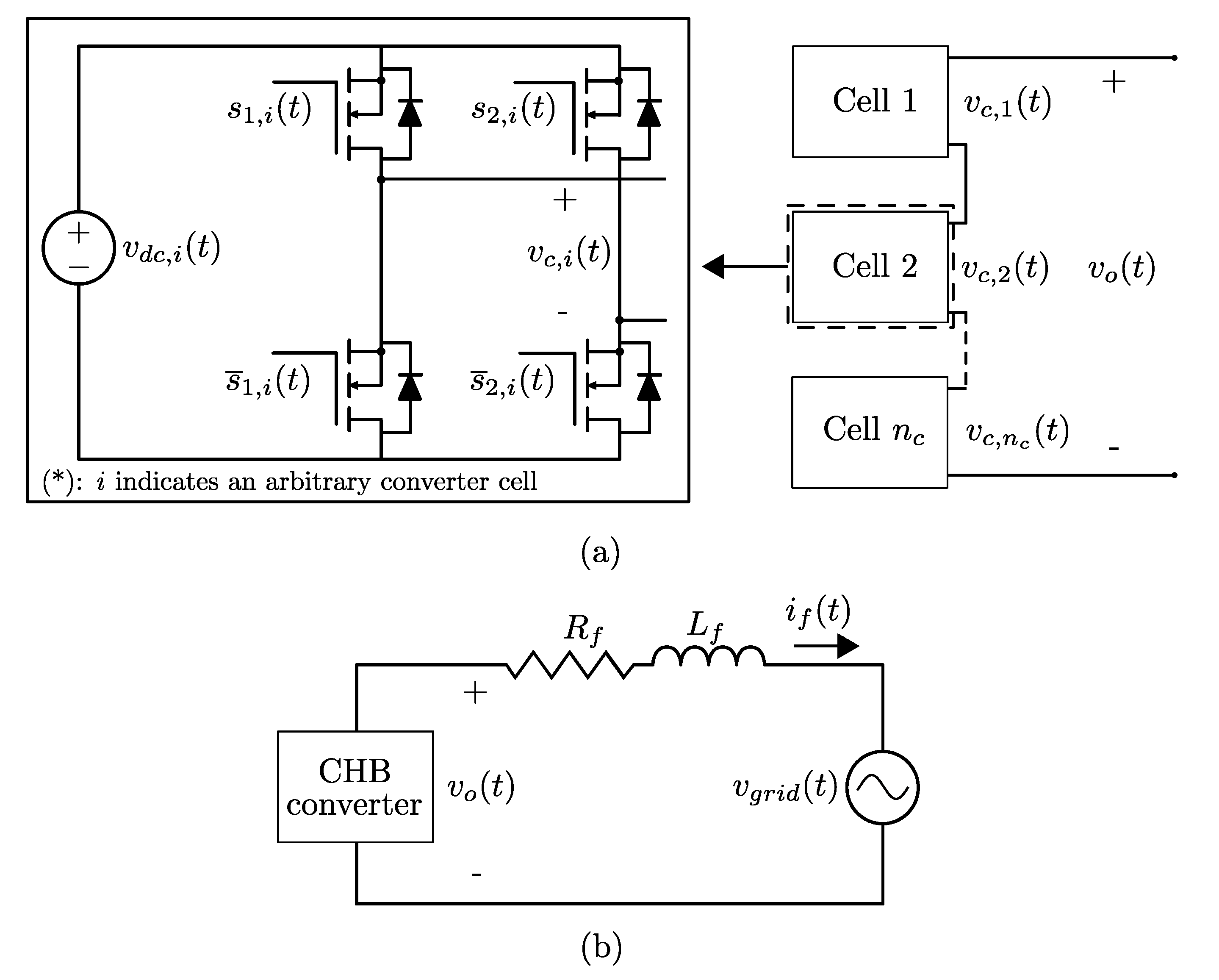
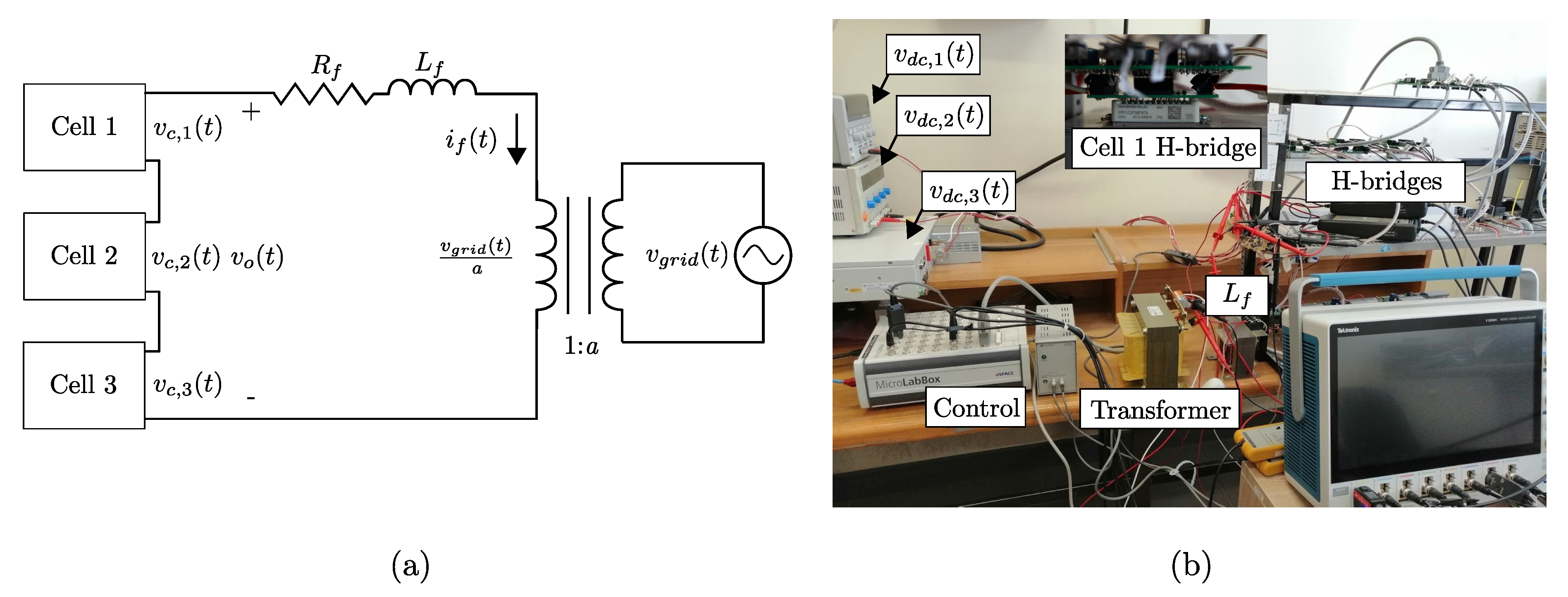
2. Cascaded H-Bridge Converter

A single-phase cascade H-bridge inverter, connected to the grid through an inductive filter, has been chosen to explain the proposed theoretical approach. The power converter system is shown in Figure 1. Throughout the paper, scalars will be denoted in italic, whereas matrices and vectors will be denoted in bold. The system model is given by the following continuous-time system:
d i f ( t ) d t = 1 L f v o ( t ) R f L f i f ( t ) 1 L f v g r i d ( t ) ,
where i f is the filter current, v o the converter output voltage, v g r i d the grid voltage, and { R f , L f } the resistance and inductance of the output filter, respectively. The output voltage v o can be rewritten as the sum of the output voltages of the n c cells which form the converter as
v o ( t ) = i = 1 n c v c , i ( t ) ,
with v c , i the output voltage of an arbitrary cell i. Because the cells are built with H-bridge inverters, their output voltage can be one of the values shown in Table 1. This output voltage can be rewritten through the switching function f H ( · ) of the H-bridge inverter and the applied state s i = s 1 , i s 2 , i T of cell i, as
v c , i ( t ) = ( s 1 , i ( t ) s 2 , i ( t ) ) v d c ( t ) = f H ( s i ) v d c ( t ) ,
with
f H ( s i ) = ( s 1 , i ( t ) s 2 , i ( t ) ) ,
and where { s 1 , i , s 2 , i } are the semiconductors’ gating signals of cell i. Replacing (3) in (2), the CHB output voltage is
v o ( t ) = i = 1 n c f H ( s i ) v d c , i ( t ) .
Equation (5) shows that the CHB output voltage is a function of the states applied to the H-bridge inside each cell. As each H-bridge can take four possible states, the CHB converter has 2 2 n c available states [25].
In order to design a discrete current controller, the system described in (1) can be discretized through the Euler forward approximation as
i ˜ f ( k + 1 ) = a d i f ( k ) + b d v o ( k ) + e d v g r i d ( k ) ,
where i ˜ f ( k + 1 ) is the estimated filter current for the sampling time k+1, and
a d = 1 T s R f L f , b d = T s 1 L f , e d = T s 1 L f .
In the following section, the discrete-time model described in (6) will be used to show the operation of conventional FCS-MPC and to propose a predictive scheme that fixes the harmonic spectra to a desired frequency.

3. Proposed Predictive Control

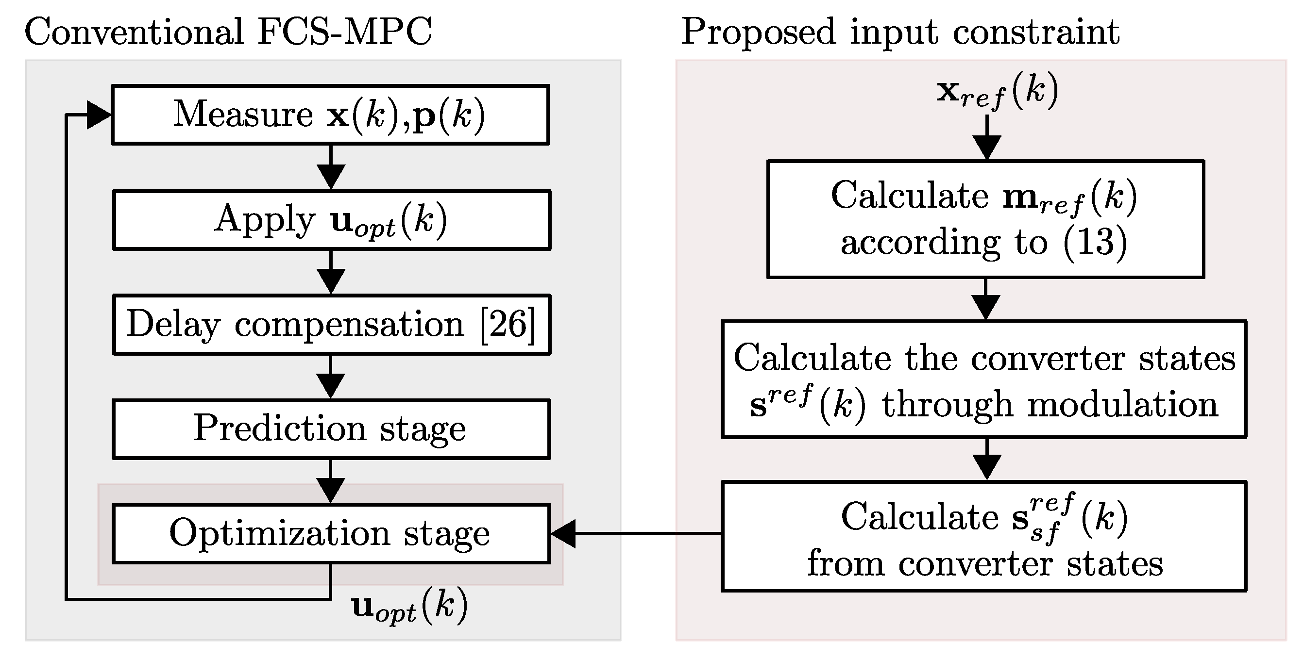
3.1. Conventional FCS-MPC

FCS-MPC schemes use a discrete-time system model to estimate future behavior within a given prediction horizon. Their objective is to identify the optimal input v o , o p t that will result in the best future performance, considering the control objectives and constraints imposed by the system. In particular, the discussion will be restricted to the simplest MPC scheme, using a prediction horizon equal to one [1,2,3,4,5,6,7]. From the discrete-time model derived in Section 2, the prediction model (6) is evaluated for each valid state of the CHB inverter. The selected state (input) is the one that allows achieving an optimum value in the desired cost function, given the imposed control objectives. In this work, the filter current tracking will be considered as a control objective. This can be expressed as
J j = ( i f , r e f ( k + 2 ) i ˜ f ( k + 2 ) ) 2 ,
where i f , r e f is the filter current reference. The input v o , o p t that generates the lowest value of (8) is applied in the next sampling time. Figure 2 shows the associated algorithm flowchart.
The described scheme shows that the controller does not have an explicit memory of the previously applied states, and therefore there is no prescribed switching pattern in the selection of the optimal state. This provokes a variable switching frequency with spread harmonic spectra [26]. Such operating conditions are not suitable for applications susceptible to problems like resonance, audible noise, semiconductor stress, and variable switching losses [9,10,11,12,13,14,15].
Several works have been proposed in the literature to reduce and/or fix the switching frequency in FCS-MPC based schemes [15,16,17,18,19,20,21,22]. Among these, the simplest proposal in terms of implementation and computational burden is shown in [16,26]. This consists in the addition of a new term in the cost function, which seeks to penalize the state change with respect to the state applied in the previous sampling time. This term can be defined as
Δ s = [ s i ( j ) s i ( k ) ] T [ s i ( j ) s i ( k ) ] ,
where s i ( j ) is one of the N available converter states and s i ( k ) is the converter state applied in the current sampling time. The resulting cost function used to track the reference current while reducing the state commutations is
J j = ( i f , r e f ( k + 2 ) i ˜ f ( k + 2 ) ) 2 + λ c Δ s ,
where λ c is the weighting factor related to the input restriction. When λ c increases, the predictive controller tends to select the same switching state applied in the previous sampling time. This reduces the number of state transitions between adjacent sampling times. However, the steady-state error increases given that the control objective associated with λ c has a higher preponderance over the control objective related to tracking error. Thus, the value of λ c is assigned by the controller designer according to the importance he gives to the input restriction.
The input restriction shown in (9) seeks to maintain the applied state for the highest number of sampling times possible. However, the input selection considers only the immediate previous state and not the complete sequence of previous inputs. This prevents the existence of a fixed switching pattern within a fundamental signal period and, consequently, a harmonic spectrum centered around a particular frequency.
To overcome these problems, this work proposes a simple predictive controller that uses the linear system model to define a new input restriction in the cost function of an FCS-MPC controller. The scheme allows for achieving a harmonic spectrum with a distribution similar to a PWM scheme without the use of multiple weighting factors or complex algorithms.

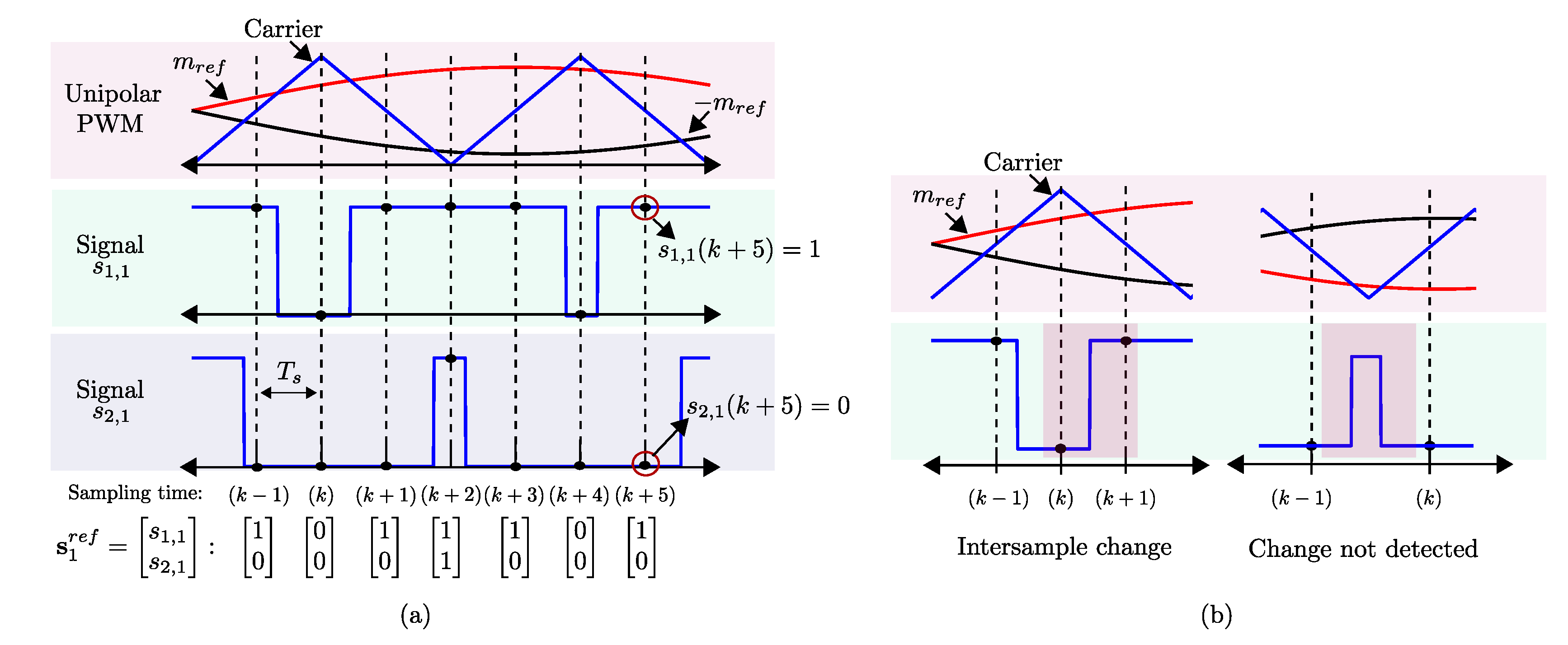
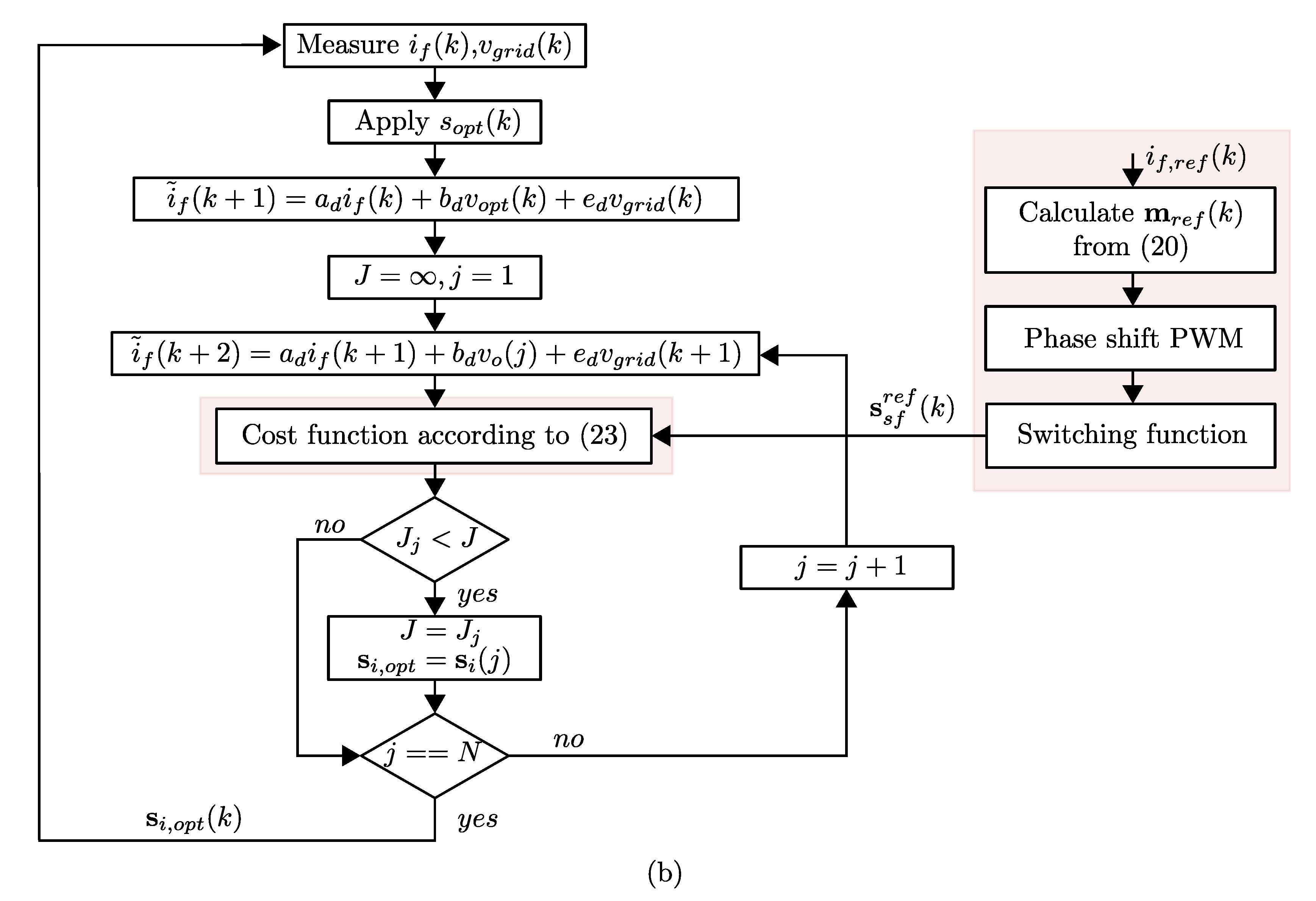
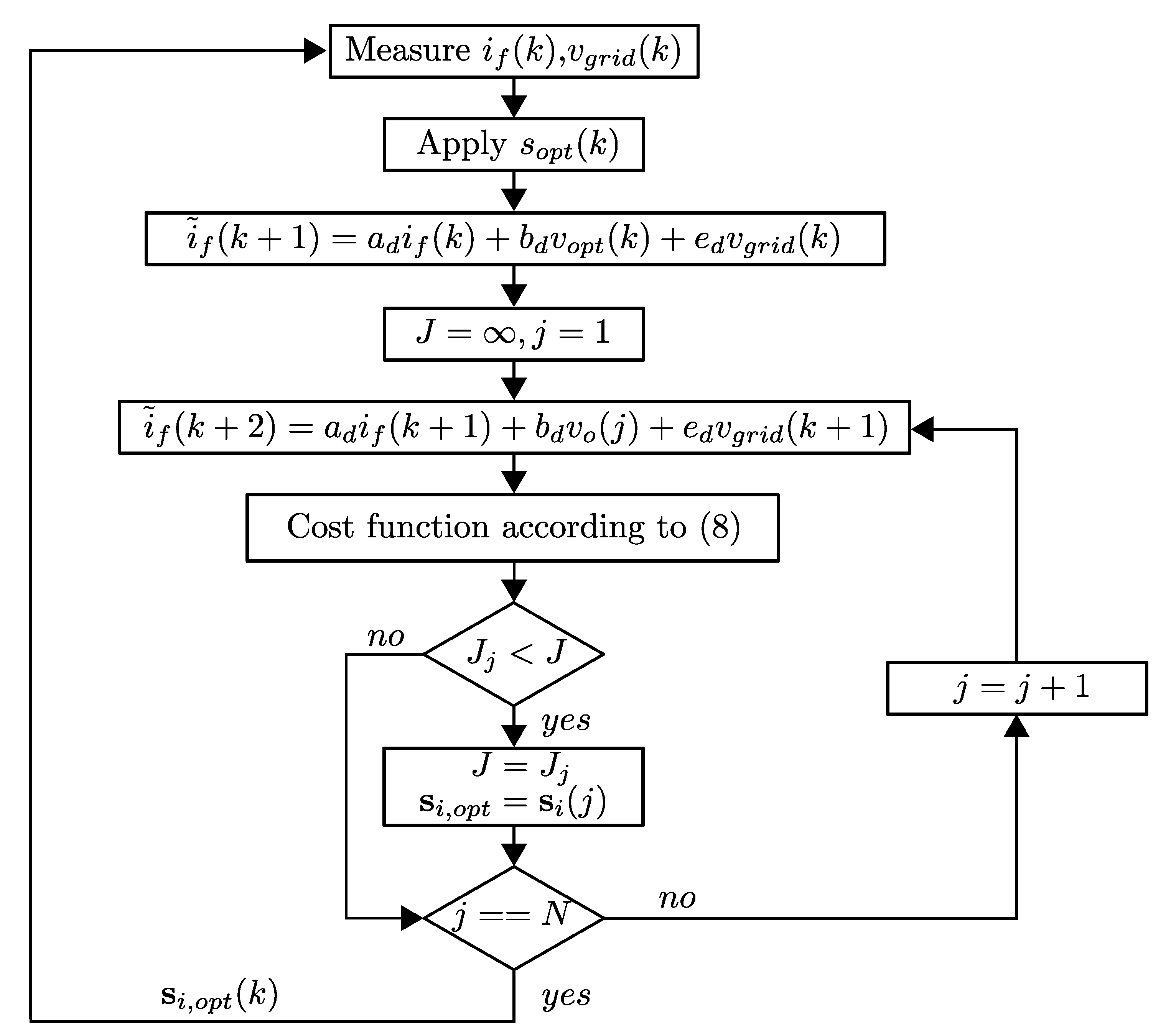
3.2. Proposed FCS-MPC

In an FCS-MPC controller, the system input is calculated in each sampling time regardless of the previously applied inputs. Thus, it is not possible to ensure a defined steady-state switching pattern to achieve a fixed switching frequency and a defined spectrum. Meanwhile, in modulated control schemes, the switching frequency and harmonic distribution are defined by the carrier signal frequency used to calculate the semiconductors’ gating signals. Despite these features, these control schemes generally have a slower dynamic response when compared to FCS-MPC schemes and need a more elaborate design process.
This section shows how it is possible to use a modulation stage to impose a fixed switching pattern on an FCS-MPC scheme, without losing its features such as fast dynamic response, optimization, and decoupled response, among others. To achieve these objectives, the proposal uses the system model (such as conventional FCS-MPC) to generate an input restriction in the FCS-MPC cost function. This restriction is calculated following the next steps:
  • Step 1:
The system model is used to calculate the converter modulator signal m r e f that allows the system to work at a steady state in the desired operating point defined by the reference. To calculate m r e f , only the fundamental component of the system variables should be considered, neglecting the switching harmonics. Consequently, the following system model at fundamental frequency is used:
x ˜ a ( k + 1 ) = A d x a ( k ) + B d u a ( k ) + E d p a ( k ) ,
where x a ( k ) , u a ( k ) , p a ( k ) are the vectors associated with the average values of the state variables, inputs, and disturbances at fundamental frequency, respectively; and the values of A d , B d , E d depend on the system parameters and sampling time T s . From (11), it is possible to calculate the input that allows the system to work at the desired operating point x r e f , a ( k ) imposed by the reference as
u a , r e f ( k ) = B d 1 ( x ˜ r e f , a ( k + 1 ) A d x r e f , a ( k ) E d p a ( k ) ) .
Finally, the converter modulator signal m r e f can be calculated from the average input u a , r e f as
m r e f ( k ) = 1 v d c ( k ) u a , r e f .
The modulator signal m r e f can be a vector or scalar depending on the number of phases of the power converter. This solution does not equal the deadbeat solution shown in [20], as (13) does not depends on the current value of the system’s variables but instead on its desired values.
  • Step 2:
The modulator reference m r e f is modulated to obtain the discrete converter inputs. This step can be implemented using standard modulation methods such as SPWM or SVM. The selected modulation method defines how the proposal fixes the value of the switching frequency; e.g., in an SPWM scheme, the switching frequency is defined by the carrier frequency. The output of this step corresponds to the converter state s r e f , formed by the gating signals to the converter’s semiconductors, which allow the system to operate in the desired operating point in steady-state.
  • Step 3:
The converter state s r e f is used to calculate the reference switching function s s f r e f associated with the power converter. This is defined as
s s f r e f ( k ) = f ( s r e f ( k ) ) ,
where f ( · ) corresponds to the converter switching function that defines the relation between the DC and AC voltage as a function of converter state, e.g., for an H-bridge converter f ( · ) is the difference between the gating signals as shown in (4). The reference switching function s s f r e f is used to generate the following input restriction in the conventional FCS-MPC scheme
Δ s p w m = i = 1 n c [ s s f r e f f ( s ( j ) ) ] T [ s s f r e f f ( s ( j ) ) ] .
Finally, the cost function used in the proposed FCS-MPC is
J j = ( x r e f ( k + 2 ) x ˜ r e f ( k + 2 ) ) T ( x r e f ( k + 2 ) x ˜ r e f ( k + 2 ) ) + λ s Δ s p w m .
Figure 3 shows a flowchart of the proposed FCS-MPC algorithm. The cost function consists of two terms: one associated with the tracking error and one to the error concerning the proposed switching function. In a transient regime, the term associated with the tracking error has a higher preponderance than the term to concentrate the harmonic spectrum. This is true, if and only if, the value of weighting factor λ s is correctly calculated. If the value of λ s is too high, the dynamic response will be defined by the term λ s Δ s p w m that corresponds to the open-loop system response. In the opposite case, if the value of λ s is too small, the dynamic response will be fast, but the system performance in steady-state will be equal to a conventional FCS-MPC controller. In a steady-state, the magnitude and phase of the tracking error are constant; therefore, the choice of the optimal state depends mainly on the term Δ s p w m . This means that, to minimize the cost function (16), the states selected by the MPC should be the closest ones to s s f r e f , which are obtained from the modulation of the m r e f signal. Thus, the switching frequency and the distribution of the harmonic spectrum are determined by the modulation stage used to generate the converter gating signals. Finally, it is assumed that the system parameters are well known, which is a reasonable assumption as the proposal works in parallel to an FCS-MPC controller that necessarily requires knowing the system parameters to ensure a good performance [26].

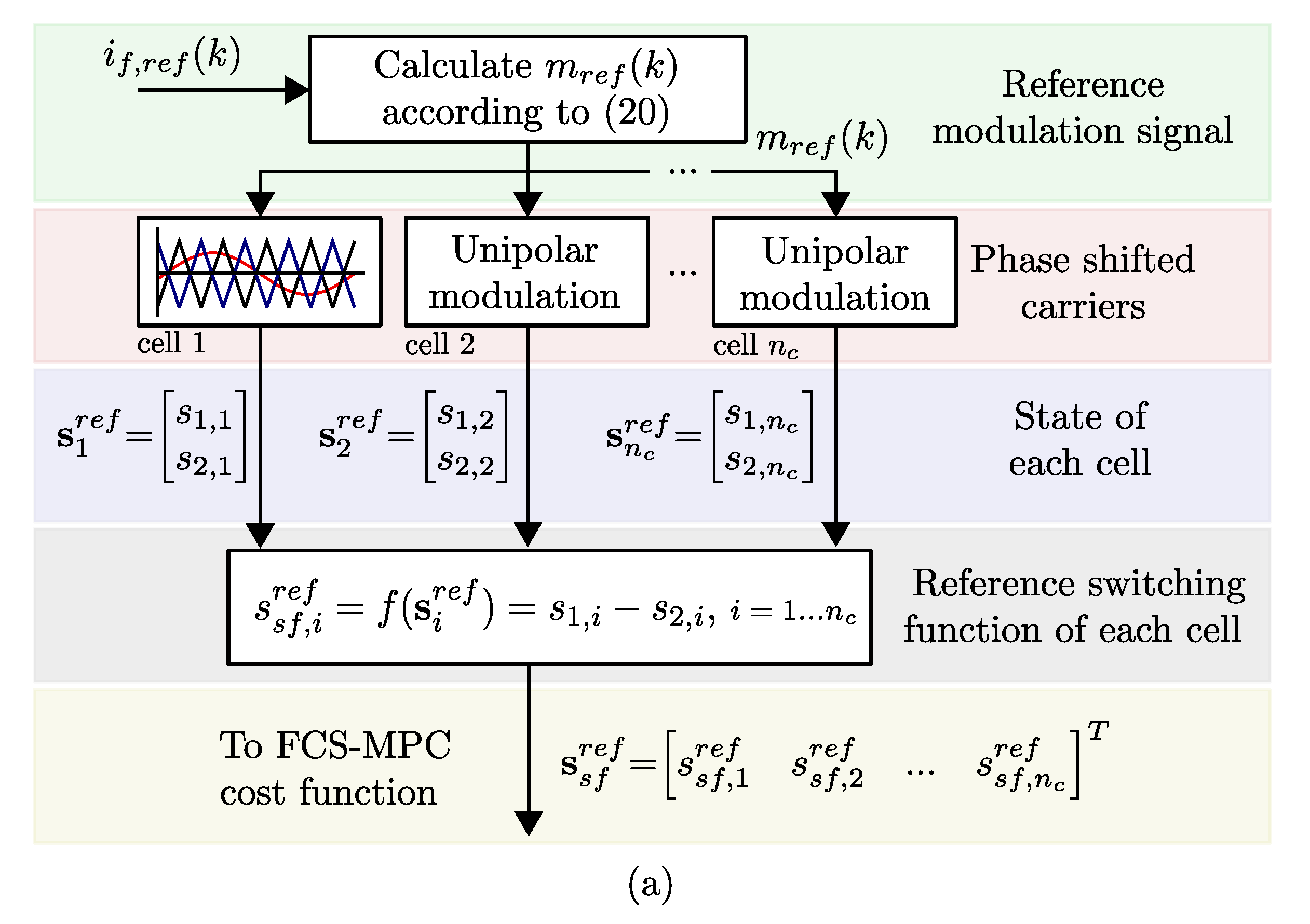
3.3. Proposed Scheme Applied to Single Phase CHB Converter

As shown in the previous section, the proposal does not change the flowchart of the conventional FCS-MPC, independently of the power converter used. This allows for using the scheme in any power converter that operates with conventional FCS-MPC. As a case study, the proposal is applied to a single-phase CHB converter, which was presented in Section 2. When an FCS-MPC algorithm is used in this converter, it is necessary to include an additional stage to ensure even power distribution among the cells [24]. Using the proposal, this feature can be naturally achieved with a fixed switching frequency and a concentrated harmonic spectrum. The steps described in Section 3.2, and applied to the CHB converter, correspond to
  • Step 1:
Using (6), it is possible to calculate the average input m r e f ( k ) that allows the system to work at the desired operating point in steady-state. Considering the average system model, it is feasible to represent the output voltage as a function of the modulation signal m ( k ) and the number of cells n c as
v o ( k ) = m ( k ) i = 1 n c v d c , i .
Replacing (17) in (6), the following expression is obtained:
i ˜ f ( k + 1 ) = a d i f ( k ) + b d m ( k ) + e d v g r i d ( k ) ,
where the DC voltages sum has been included in b d and the system variables now represent their average values. From (18), m ( k ) can be rewritten as a function of state variables and system disturbance as
m ( k ) = b d 1 ( i ˜ f ( k + 1 ) a d i f ( k ) e d v g r i d ( k ) ) .
Finally, it is expected in steady-state that the filter current be equal to the desired reference, hence (19) can be rewritten as
m r e f ( k ) = b d 1 ( i ˜ f , r e f ( k + 1 ) a d i f , r e f ( k ) e d v g r i d ( k ) ) ,
where the filter current i f has been replaced by the desired filter current reference on steady-state and the input m ( k ) has been renamed as m r e f . This corresponds to the average input that allows the system in steady-state to work at the desired operating point.
  • Step 2:
The modulation signal calculated in (20) is modulated through phase-shift PWM (PSPWM). This modulation technique allows an even power distribution among cells if the DC voltage of each one are equal [23]. The output of this step corresponds to the firing signals { s 1 , i , s 2 , i } associated with the semiconductors of cell i, as an example, Figure 4a shows the calculation of the semiconductor’s gating signals for the cell 1. In each sampling time, the values of the signals s 1 , 1 and s 2 , 1 are calculated and used to generate the state vector s 1 r e f .
The comparison between m r e f and the carrier signal can generate at most two transitions in each signal s 1 , 1 and s 2 , 1 . Because these signals are sampled or calculated each sampling time, it is possible that there are one or two transitions between samples if the sampling time is high (Figure 4b). When one transition occurs in the middle of a sampling time, its value will be naturally considered in the next sampling time. In the proposal, one change between samples is not a problem because the strategy is not allowed to change between samples as an FCS-MPC controller is used (its output can only change at the sampling times). When two transitions occur, the switching function associated with the cell will be the same in two consecutive sampling times. This condition is a problematic issue because the proposal seeks to impose a PWM waveform, and losing pulses results in changes in the desired harmonic spectrum. However, both issues can be avoided increasing the ratio between the sampling and carrier frequency, e.g., for a carrier frequency of 550 Hz and a sampling time of 10 kHz, there are 18 samples per carrier period, which translates to a resolution of 0.1 ms.
  • Step 3:
The reference switching function of each cell is calculated as
s s f , i r e f = f H ( s i r e f ) = s 1 , i s 2 , i ,
with { s 1 , i , s 2 , i } the gating signals of an arbitrary cell i calculated in step 2. Then, the following input restriction on the conventional FCS-MPC cost function can be calculated:
Δ s p w m = i = 1 n c ( s s f , i r e f f H ( s ( j ) ) ) 2 ,
where j is one of the N states of the power converter evaluated in the cost function. Finally, the cost function implemented is
J = ( i f , r e f ( k + 2 ) i f ( k + 2 ) ) 2 + λ s Δ s p w m .
The resulting algorithm is shown in Figure 5. In each sampling time, the FCS-MPC controller selects the state that minimizes the cost function J. Because in a steady-state, it is expected that the reference tracking term is close to zero, and the selected state will depend mainly on the proposed input restriction. Thus, the FCS-MPC controller will select the state that generates the closest converter switching function to the one proposed by the input restriction.

4. Experimental Results

The experimental set-up used to test the proposal corresponds to a grid-connected single-phase CHB, Figure 6. Each cell of this converter was built with an H-bridge module FPF1C2P5BF07A fed by a constant DC source. The CHB converter is connected to the grid through an inductive filter and a link transformer. The system parameters are shown in Table 2.
The FCS-MPC algorithms were implemented in a dSpace MicroLabBox with a sampling frequency f s of 10 kHz. In the case of the proposal, a carrier frequency of 11 per unit (p.u.) was selected, which allows for fixing the harmonic spectrum at 22 p.u. The H-bridge modules were modulated using unipolar SPWM. The weighting factors used in the proposed FCS-MPC controller were calculated using the branch and bound method described in [26,27].
The stationary and transient response of the proposed algorithm is compared with the response of a conventional scheme using a strategy to achieve even power distribution among cells [24]. First, experimental tests in the steady state were performed to compare the harmonic spectra and average switching frequency per semiconductor (ASF) of the conventional strategy with the proposed strategy. For comparison purposes, the ASF of both schemes is compared with the achieved using an ideal modulation scheme with the same carrier frequency as the proposal. The ASF for a carrier frequency of 11 p.u. is 1.1 kHz. Afterwards, the dynamic response of both strategies is tested for a step-change in the output current reference from 1.5 A to 3.5 A. Finally, the response of the system under a parameter mismatch of 100% is presented for the conventional and proposed schemes.

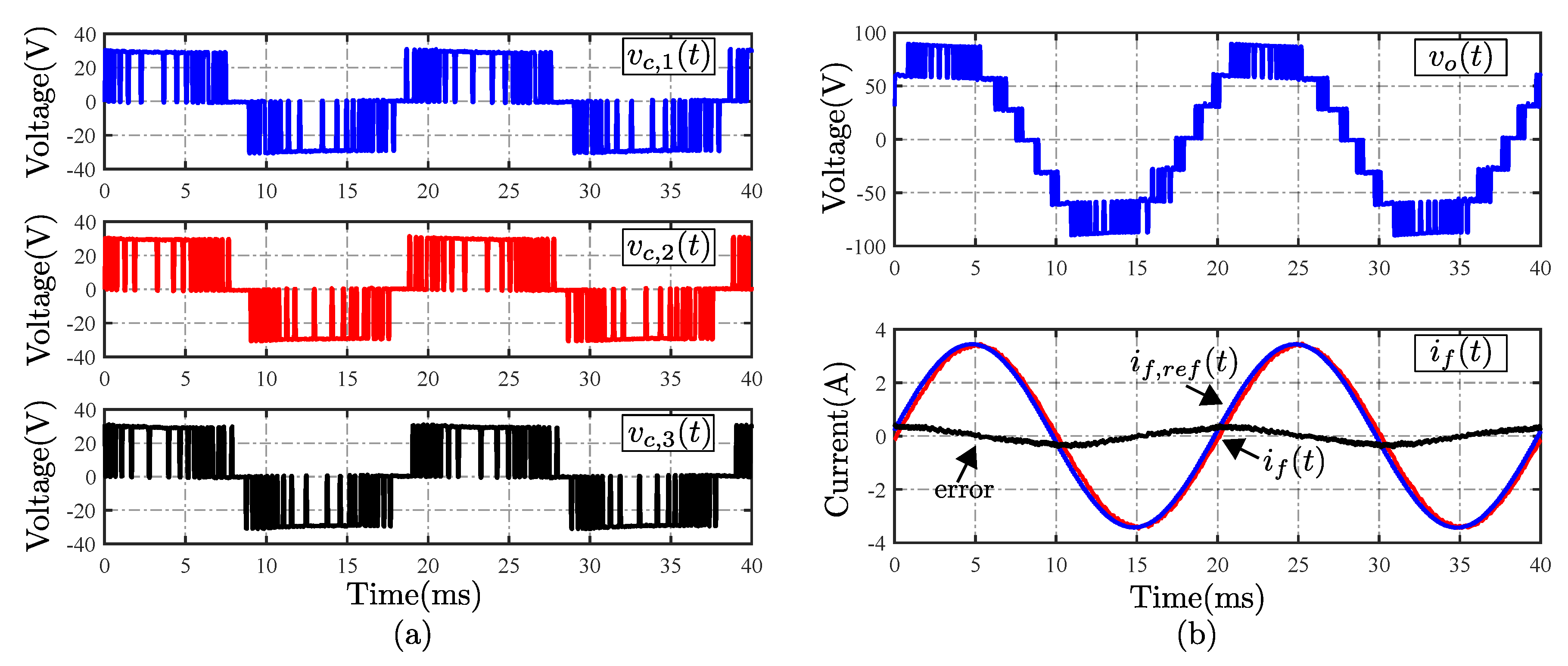
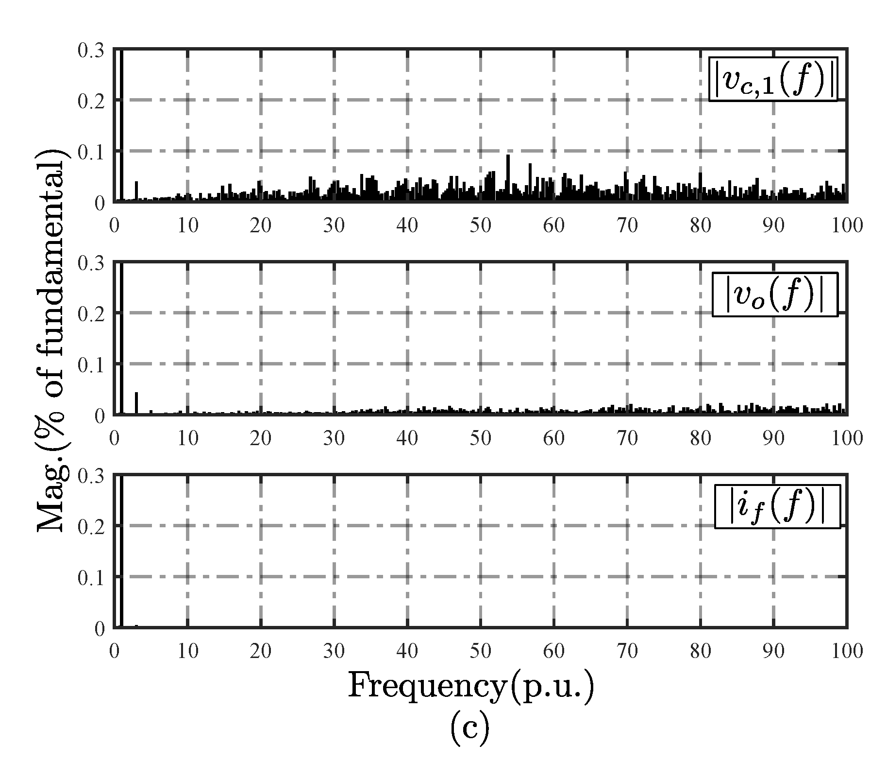
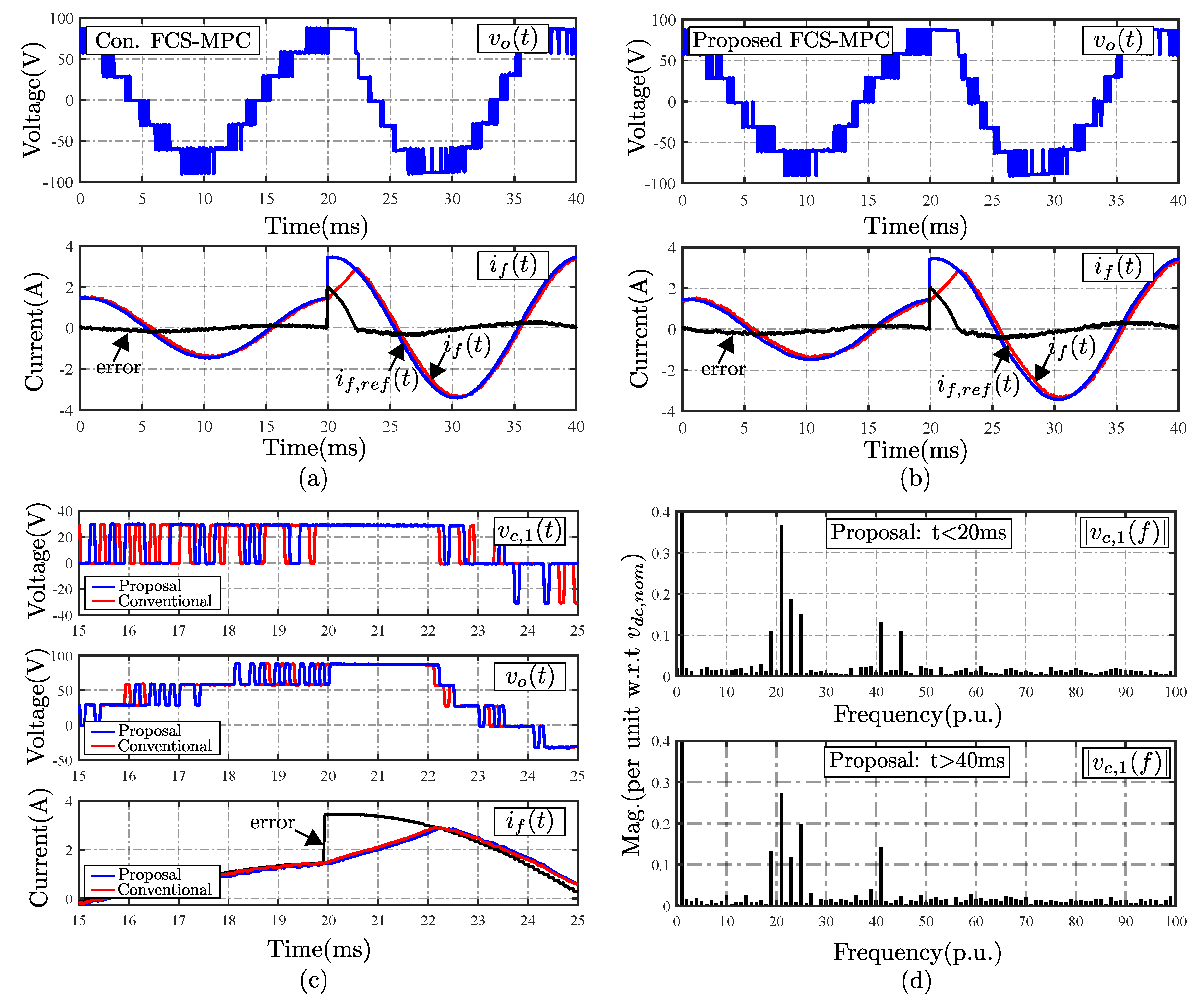
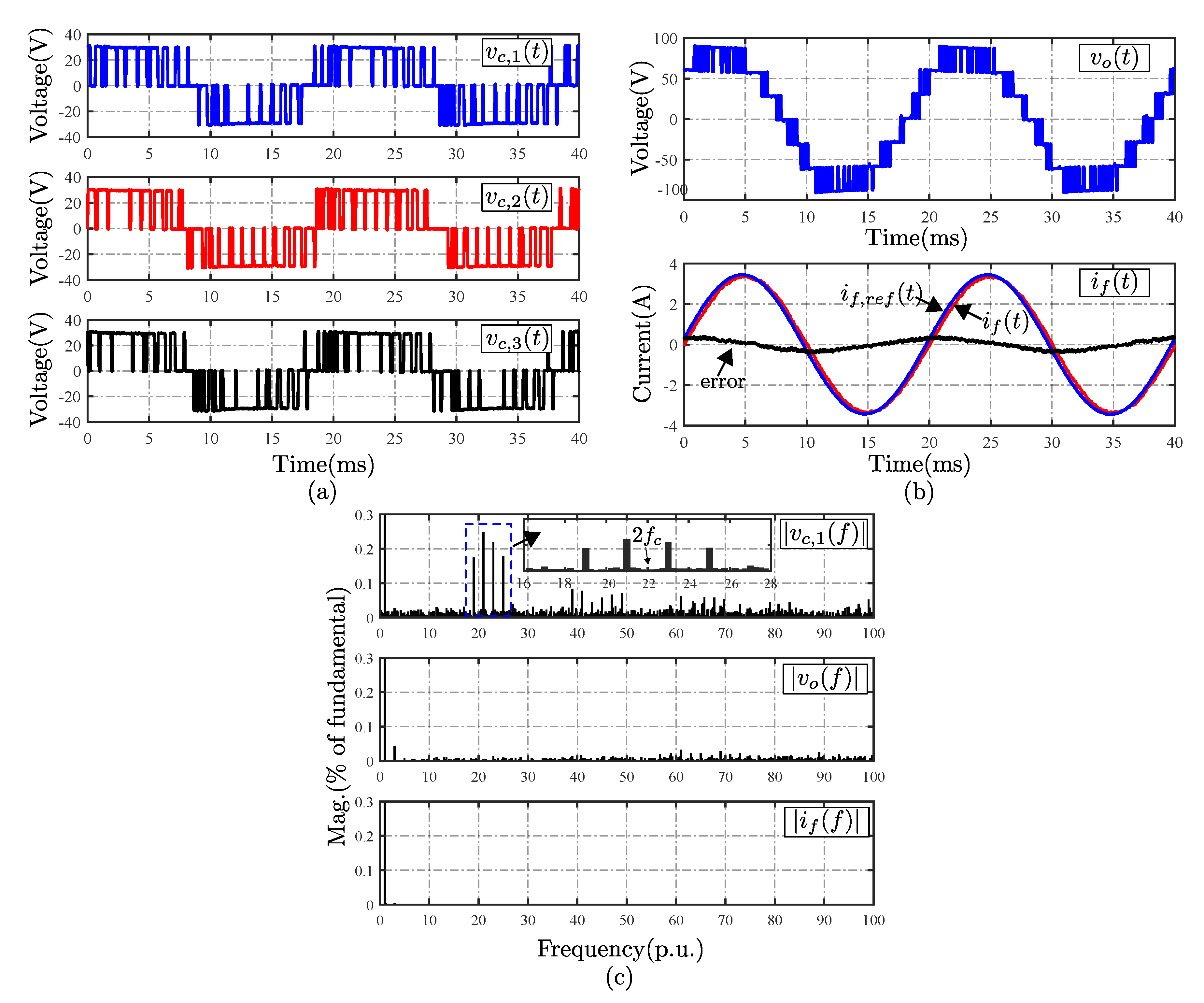
4.1. Steady-State Performance

Figure 7 shows the steady-state performance of the system with conventional FCS-MPC for a current reference of 3.5 A. The average value of each cell output voltage is similar among them, due to the use of the strategy presented in [24], Figure 7a. These values are summarized in Table 3. The sum of these voltages generate the typical 7-level waveform in the output of the CHB converter, Figure 7b; while the current tracks the reference with an error of 4.85% at the fundamental frequency. Figure 7c shows the typical spread spectrum obtained with a conventional MPC scheme, with concentrations around f s /11 and f s /6. The average switching frequency per semiconductor (ASF) is equal to 1.97 kHz, which is 79.6% higher than the achieved using a modulated scheme with a carrier frequency of 11 p.u.
Figure 8 shows the steady-state performance of the proposal operating with a carrier frequency of 11 p.u. The fundamental output voltage of each cell is similar (Table 3), Figure 8a, with a converter output voltage of 7-levels as the conventional FCS-MPC, Figure 8b. The output current follows the reference with an error at the fundamental frequency of 5.71%. Figure 8c shows the key harmonic spectra for the proposed FCS-MPC. The proposal allows for obtaining a well-defined harmonic spectrum around twice the carrier frequency for the cell output voltage—while, in the case of total output voltage, the harmonics are concentrated around six times the carrier frequency, due to the phase shift modulation used. The average switching frequency of the proposal is 1.2 kHz, which is 40% less than conventional scheme and 9% higher than a modulated scheme with the same carrier frequency.
Table 4 shows the associated THD for both controllers studied. The results show that the proposed method has a higher THD than conventional FCS-MPC because the harmonic spectrum of the proposal is closer to the filter cut-off frequency. Although the THD increases, the system still works with low current distortion, a fixed harmonic spectrum, an even power distribution, and can operate with a lower average switching frequency than conventional FCS-MPC.

4.2. Dynamic Performance

The proposed strategy is tested for a step-change in the current reference of 133%, from 1.5 A to 3.5 A at t = 20 ms, as shown in Figure 9. The conventional and proposed FCS-MPC show a similar dynamic performance, which can be seen in Figure 9a,b, respectively. This can be inferred by comparing the output voltage applied by the CHB converter in both cases. For instance, the results of Figure 9c show that, immediately after the current step-change, both strategies select the same voltage vector. Finally, Figure 9d shows the voltage harmonic spectrum for the proposal associated with cell number 1, before and after the current change. It can be seen that the proposal allows for fixing the harmonic spectrum around twice the carrier frequency, independently of the change on the system operating point and without requiring to change the associated weighting factor.

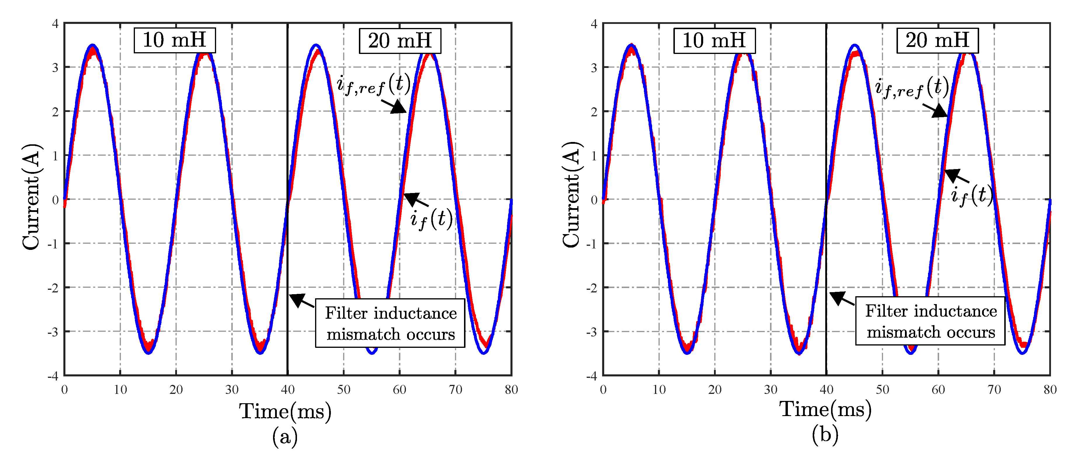
4.3. Parameter Sensitivity

In this section, the sensitivity of the conventional and proposed FCS-MPC under a change of 50% in the inductance value is evaluated. The change is made at t = 40 ms from an inductance value of 10 mH to 20 mH while the current reference is set at 3.5 A. The initial value of the inductance used for both FCS-MPC algorithms is 10 mH. The results achieved for this test are shown in Figure 10. The conventional scheme tracks the reference, despite the change in the inductance value, with an error at fundamental frequency of 0.15 A before the change and 0.17 A when the inductance value is 20 mH, Figure 10a. In the case of the proposal, Figure 10b, the error at 50 Hz before and after the change are 0.1 A and 0.2 A, respectively. These results show that the proposal allows for fixing the harmonic spectrum and switching frequency, without considerably altering the conventional FCS-MPC performance under parameter mismatch.

5. Discussion

Conventional FCS-MPC schemes have drawbacks related to the variable switching frequency when used on static power converters. One of them is their characteristic spread spectrum, which, depending on the application, can make it an unsuitable strategy [9,10,11,12,13,14,15]. A variety of strategies have been proposed to improve the switching characteristics in converters that use FCS-MPC [16,17,18,19,20,21,22]. In order to achieve control schemes that concentrate the harmonic spectrum, the previous approaches allow for defining the switching frequency at the cost of more complex algorithms, either increasing the model dependence, or sacrificing the characteristics that distinguish direct predictive control from modulation-based schemes.
The proposed scheme includes an input constraint that, in contrast to [16], does not seek to penalize the state change with respect to the previous input. Instead, it seeks to penalize the state change with respect to the optimum obtained from the modulation of the input calculated by (20); which corresponds to the required input in steady state to track the imposed reference. Greater weight is placed on the input constraint by increasing the value of λ s , in other words, to the state obtained from the modulation stage. However, given that this state is an optimum one for that particular sampling instant, there is no degradation to the current tracking due to the selection of this input. In the case of a conventional input constraint, as the objective is not to change the input, it is not possible to ensure that the input applied in the last sampling instant minimizes the cost function in the current sampling time, increasing the tracking error of the desired variables.
The experimental results show that the proposal allows for achieving a concentrated spectrum in a steady state, similar to a PWM scheme, and a dynamic performance such as the one obtained with a conventional FCS-MPC strategy. In addition, it has a similar performance when compared to the conventional case in terms of error at fundamental frequency. While the proposal has an error of 5.71%, the conventional case has an error of 4.78%. This increase is produced because the FCS-MPC controller must select the state based on two control objectives. In other words, the selected state is not necessarily the same optimal state as when only the reference tracking control objective is used. The same argument explains the behavior when parameter mismatch is present, where both strategies show a similar performance, but the proposal shows a slight increment in the error at fundamental frequency.
The implementation of the proposal requires calculating or measuring the outputs of the modulation stage each sampling time to perform the proposed input restriction. As the measurements are made at intervals multiples of T s , the resulting PWM pattern (in a fundamental period) is equal to the one obtained when comparing the signal m r e f with a carrier signal generated by software with a resolution of f s / f c . This means that the harmonic distribution achieved with the proposal depends on the resolution of the carrier signal, or equivalently, its ratio with respect to the sampling frequency. Thus, for a higher carrier signal resolution, a better representation of the PWM pattern and, consequently, a closer harmonic spectrum to the one of a modulated scheme.
In terms of computational burden, the proposed scheme has a computation time of 13.3 us, which is 0.7% (just 0.1 us) higher than the conventional FCS-MPC using [24] (13.2 us). The additional time is due mostly to the calculation of the triangular signal (via a look-up table) and the input at fundamental frequency m r e f ; both signals are required to calculate the proposed input restriction. However, this time can be improved because it depends on the used hardware, the modulation scheme selected, and on how the required signals are calculated.
The disadvantages of the proposed scheme are related to: (i) the availability of a representative model of the system, and (ii) the capacity of the hardware required to obtain an adequate resolution for the carrier signal. In the first case, like any predictive control strategy, it is necessary to have a good representative model to operate the control scheme correctly. In the second case, the resolution of the carrier signal is subjected to the required frequency to set the harmonic spectrum. In the second case, the sampling frequency used depends on the carrier signal frequency. The experimental results were obtained using a sampling frequency of 10 kHz for a carrier frequency of 550 Hz which results in a carrier resolution of 18 point per period (0.1 ms). The sampling time must be selected in order to mitigate or avoid the problems described in Figure 4b regarding the resolution of the PWM signal used to create the input restriction. Hence, a good selection of the ratio between the sampling frequency and carrier frequency ( f s / f c ) ensures a harmonic spectrum closest to the one achieved with a modulated scheme. A high ratio allows for a good representation of the PWM signal, while a small ratio, such as the minimal theoretically acceptable by the Nyquist frequency ( f s / f c = 2 ), may not be sufficient to detect a change in the PWM signals. The selection of the sampling frequency also depends on the available hardware used for implementation, as a high sampling frequency reduces the time available for the algorithm’s execution.
Finally, a comparison between the proposed strategy and previous schemes can be observed in Table 5. In this table, characteristics like dynamic response, optimization, and spread spectrum, among others, are compared for different FCS-MPC control schemes. These features allow a qualitative comparison of them.

6. Conclusions

This work has introduced a new approach to mitigating spread spectrum harmonics and fixing the switching frequency in conventional FCS-MPC schemes. The implemented strategy allows for obtaining a harmonic spectrum similar to that achieved by a PWM strategy with unipolar modulation. The proposed control scheme presents a competitive dynamic performance, comparable to that obtained by conventional predictive control, through a simple and intuitive implementation that requires neither increased computation burden nor a formal modulation stage to apply the states of the converter. The strategy has been evaluated under a variety of operating conditions in a grid-connected CHB inverter. Experimental results demonstrate a satisfactory steady-state performance with an even power distribution among cells, with a reduced average switching frequency and a fixed harmonic spectrum.

Author Contributions

Analysis, investigation and validation, R.O.R. and C.R.B.; writing—original draft preparation, R.O.R. and F.V.; supervision, J.E. and C.R.B. All authors have read and agreed to the published version of the manuscript.

Funding

This work was supported by the FONDECYT Project 1201308, Project ANID/FONDAP/15110019 and CONICYT/DOCTORADO NACIONAL/21160928.

Conflicts of Interest

The authors declare no conflict of interest.

References

  1. Cortes, P.; Kazmierkowski, M.P.; Kennel, R.M.; Quevedo, D.E.; Rodriguez, J. Predictive control in power electronics and drives. IEEE Trans. Ind. Electron. 2008, 55, 4312–4324. [Google Scholar] [CrossRef]
  2. Roberts, P.D. A brief overview of model predictive control. In Proceedings of the IEEE Seminar on Practical Experiences with Predictive Control, Middlesbrough, UK, 16 February 2000; Volume 55, pp. 1–3. [Google Scholar]
  3. Lee, J.H. Model predictive control: Review of the three decades of development. Int. J. Control Autom. Syst. 2011, 9, 415–424. [Google Scholar] [CrossRef]
  4. Rodriguez, J.; Kazmierkowski, M.P.; Espinoza, J.R.; Zancheta, P.; Abu-Rub, H.; Young, H.A.; Rojas, C.A. State of the art of finite control set model predictive control in power electronics. IEEE Trans. Ind. Inf. 2013, 9, 1003–1016. [Google Scholar] [CrossRef]
  5. Huang, J.; Yang, B.; Guo, F.; Wang, Z.; Tong, X.; Zhang, A.; Xiao, J. Priority sorting approach for modular multilevel converter based on simplified model predictive control. IEEE Trans. Ind. Electron. 2018, 65, 4819–4830. [Google Scholar] [CrossRef]
  6. Aguilera, R.; Lezana, P.; Quevedo, D. Switched model predictive control for improved transient and steady-state performance. IEEE Trans. Ind. Inf. 2015, 11, 968–977. [Google Scholar] [CrossRef]
  7. Kouro, S.; Cortes, P.; Vargas, R.; Ammann, U.; Rodriguez, J. Model predictive control -A simple and powerful method to control power converters. IEEE Trans. Ind. Electron. 2009, 56, 1826–1838. [Google Scholar] [CrossRef]
  8. Sandre-Hernandez, O.; Rangel-Magdaleno, J.; Morales-Caporal, R. A comparison on finite-set model predictive torque control schemes for PMSMs. IEEE Trans. Ind. Electron. 2018, 33, 8838–8847. [Google Scholar] [CrossRef]
  9. Patsakis, G.; Karamanakos, P.; Stolze, P.; Manias, S.; Kennel, R.; Mouton, T. Variable switching point predictive torque control for the four-switch three-phase inverter. In Proceedings of the IEEE International Symposium on Sensorless Control for Electrical Drives and Predictive Control of Electrical Drives and Power Electronics, Munich, Germany, 17–19 October 2013; Volme 33, pp. 1–8. [Google Scholar]
  10. Acuna, P.; Aguilera, R.; Ghias, A.; Rivera, M.; Baier, C.; Agelidis, V. Cascade-Free Model Predictive Control for Single-Phase Grid-Connected Power Converters. IEEE Trans. Ind. Electron. 2017, 64, 285–294. [Google Scholar] [CrossRef]
  11. Ramírez, R.; Espinoza, J.; Baier, C.; Rivera, M.; Villarroel, F.; Guzman, J.; Melín, P. Finite-State Model Predictive Control with Integral Action Applied to a Single-Phase Z-Source Inverter. IEEE J. Emerg. Sel. Top. Power Electron. 2019, 7, 228–239. [Google Scholar] [CrossRef]
  12. Ge, H.; Zhen, Y.; Wang, Y.; Wang, D. Research on LCL filter active damping strategy in active power filter system. In Proceedings of the International Conference on Modelling, Identification and Control, Kunming, China, 10–12 July 2017; pp. 476–481. [Google Scholar]
  13. Fang, J.; Xiao, G.; Yang, X.; Tang, Y. Parameter design of a novel series-parallel-resonant LCL filter for single-phase half-bridge active power filters. IEEE Trans. Power Electron. 2017, 32, 200–217. [Google Scholar] [CrossRef]
  14. Ferreira, S.; Gonzatti, R.; Pereira, R.; da Silva, C.; da Silva, L.; Lambert-Torres, G. Finite control set model predictive control for dynamic reactive power compensation with hybrid active power filters. IEEE Trans. Power Electron. 2018, 65, 2608–2617. [Google Scholar] [CrossRef]
  15. Geldenhuys, J.; du Toit Mouton, H.; Rix, A.; Geyer, T. Model predictive current control of a grid connected converter with LCL-filter. In Proceedings of the IEEE Workshop on Control and Modeling for Power Electronics (COMPEL), Trondheim, Norway, 27–30 June 2016; pp. 1–6. [Google Scholar]
  16. Yaramasu, V.; Rivera, M.; Wu, B.; Rodriguez, J. Model predictive current control of two-level four-leg inverters—Part I: Concept, algorithm, and simulation analysis. IEEE Trans. Power Electron. 2013, 28, 3459–3468. [Google Scholar] [CrossRef]
  17. Aguirre, M.; Kouro, S.; Rojas, C.; Rodriguez, J.; Leon, J. Switching frequency regulation for FCS-MPC based on a period control approach. IEEE Trans. Power Electron. 2018, 65, 5764–5773. [Google Scholar] [CrossRef]
  18. Tarisciotti, L.; Zanchetta, P.; Watson, A.; Clare, J.; Degano, M.; Bifaretti, S. Modulated Model Predictive Control for a Three-Phase Active Rectifier. IEEE Trans. Ind. Appl. 2015, 51, 1610–1620. [Google Scholar] [CrossRef]
  19. Donoso, F.; Mora, A.; Cardenas, R.; Angulo, A.; Sáez, D.; Rivera, M. Finite-Set Model-Predictive Control Strategies for a 3L-NPC Inverter Operating With Fixed Switching Frequency. IEEE Trans. Ind. Electron. 2018, 65, 3954–3965. [Google Scholar] [CrossRef]
  20. Liu, X.; Wang, D.; Peng, Z. Cascade-Free Fuzzy Finite-Control-Set Model Predictive Control for Nested Neutral Point-Clamped Converters With Low Switching Frequency. IEEE Trans. Control Syst. Technol. 2019, 27, 2237–2244. [Google Scholar] [CrossRef]
  21. Zhang, Y.; Liu, J.; Yang, H.; Fan, S. New Insights into Model Predictive Control for Three-Phase Power Converters. IEEE Trans. Ind. Appl. 2019, 55, 1973–1982. [Google Scholar] [CrossRef]
  22. Gong, Z.; Wu, X.; Dai, P.; Zhu, R. Modulated Model Predictive Control for MMC-Based Active Front-End Rectifiers Under Unbalanced Grid Conditions. IEEE Trans Ind. Electron. 2019, 66, 2398–2409. [Google Scholar] [CrossRef]
  23. Malinowski, M.; Gopakumar, K.; Xu, D.; Rodriguez, J.; Pérez, M.A. A Survey on Cascaded Multilevel Inverters. IEEE Trans. Ind. Electron. 2010, 57, 2197–2206. [Google Scholar] [CrossRef]
  24. Wilson, A.; Cortés, P.; Kouro, S.; Rodriguez, J.; Abu-Rub, H. Model predictive control for cascaded h-bridge multilevel inverters with even power distribution. In Proceedings of the IEEE International Conference on Industrial Technology, Vina del Mar, Chile, 14–17 March 2010; Volume 57, pp. 1271–1276. [Google Scholar]
  25. Cortés, P.; Wilson, A.; Kouro, S.; Rodriguez, J.; Abu-Rub, H. Model Predictive Control of Multilevel Cascaded H-Bridge Inverters. IEEE Trans. Ind. Electron. 2010, 57, 2691–2699. [Google Scholar] [CrossRef]
  26. Karamanakos, P.; Geyer, T. Guidelines for the Design of Finite Control Set Model Predictive Controllers. IEEE Trans. Ind. Electron. 2020, 7, 7434–7450. [Google Scholar] [CrossRef]
  27. Cortés, P.; Kouro, S.; La Rocca, B.; Vargas, R.; Rodríguez, J.; León, J.I.; Vazquez, S.; Franquelo, L.G. Guidelines for weighting factors design in Model Predictive Control of power converters and drives. In Proceedings of the 2009 IEEE International Conference on Industrial Technology, Gippsland, Australia, 10–13 February 2009; pp. 1–7. [Google Scholar]
  28. Cortes, P.; Rodriguez, J.; Quevedo, D.; Silva, C. Predictive Current Control Strategy With Imposed Load Current Spectrum. IEEE Trans. Ind. Electron. 2007, 23, 612–618. [Google Scholar]
Figure 1. Cascade H-bridge converter. (a) standard topology; (b) grid connected single phase CHB.
Energies 13 05475 g001
Figure 2. Conventional FCS-MPC flowchart applied to a grid-connected CHB inverter.
Energies 13 05475 g002
Figure 3. Proposed FCS-MPC. Red boxes indicate new or modified stages.
Energies 13 05475 g003
Figure 4. Proposed FCS-MPC applied to grid-connected CHB inverter. Modulation stage. (a) Calculation of s 1 r e f ; (b) sampling time issues.
Energies 13 05475 g004
Figure 5. Proposed FCS-MPC applied to grid-connected CHB inverter. (a) input restriction generation; (b) proposed algorithm flowchart where the red label indicates new or modified stages.
Energies 13 05475 g005aEnergies 13 05475 g005b
Figure 6. System used for the experimental tests. (a) electrical diagram; (b) experimental setup.
Energies 13 05475 g006
Figure 7. Experimental results for conventional FCS-MPC [24]. (a) cell voltage; (b) output voltage and current; (c) key-waveforms harmonic spectra.
Energies 13 05475 g007aEnergies 13 05475 g007b
Figure 8. Experimental results for proposed FCS-MPC. (a) cells voltage; (b) output voltage and current; (c) key-waveforms harmonic spectra.
Energies 13 05475 g008
Figure 9. Experimental results for a current reference step-change from 1.5 A to 3.5 A. (a) conventional FCS-MPC [24]; (b) proposed FCS-MPC; (c) voltage states (zoom); (d) cell 1 voltage spectrum, before and after the change.
Energies 13 05475 g009
Figure 10. Experimental results for a step-change of +100% from 10 mH to 20 mH on the filter inductance value at t = 40 ms. (a) conventional FCS [24]; (b) proposed FCS.
Energies 13 05475 g010
Table 1. Admissible states for H-Bridge inverter.
s 1 s 2 v o
10+ v d c
000
110
01 v d c
Table 2. System’s parameters.
FeaturesDescriptionValue
v d c Cells DC voltage30 V
v g r i d Grid voltage120 V
R f Filter resistance0.6 Ω
L f Filter inductance20 mH
f g r i d Grid frequency50 Hz
f s Sampling frequency10 kHz
f c Carrier frequency550 Hz
Table 3. Fundamental cell voltages (50 Hz) p.u. w.r.t DC voltage.
VoltageConventional FCS-MPC [24]Proposed FCS-MPC
v c , 1 0.9290.959
v c , 2 0.9310.935
v c , 3 0.9370.935
v o 2.7972.829
Table 4. Key waveforms THD% until harmonic 51 p.u.
SignalConventional FCS-MPC [24]Proposed FCS-MPC
v c , 1 32.3249.22
v c , 2 33.1647.78
v c , 3 30.9047.19
v o 9.9210.34
i f 1.041.32
Table 5. Comparison among classical linear controller, proposed scheme and previous FCS solutions.
FeatureConventional FCS-MPCProposed FCS-MPCPeriod Control [17]M2PC [18]Notch Filter [28]
Switching frequency depends ofSampling frequencyCarrier ✓ frequencyWeighting factor tuningSVM frequencyFilter tuning
Dynamic responseFast ✓Fast ✓Fast ✓Fast ✓Medium
Spread spectrumHighLow ✓MediumMediumLow ✓
ImplementationSimple ✓Simple ✓MediumMediumMedium
Even power distribution (CHB case)NoYes ✓NoYes ✓No
Publisher’s Note: MDPI stays neutral with regard to jurisdictional claims in published maps and institutional affiliations.

