Abstract
The paper presents an application of the homotopy analysis method for solving the one-phase fractional inverse Stefan design problem. The problem was to determine the temperature distribution in the domain and functions describing the temperature and the heat flux on one of the considered area boundaries. It was demonstrated that if the series constructed for the method is convergent then its sum is a solution of the considered equation. The sufficient condition of this convergence was also presented as well as the error of the approximate solution estimation. The paper also includes the example presenting the application of the described method. The obtained results show the usefulness of the proposed method. The method is stable for the input data disturbances and converges quickly. The big advantage of this method is the fact that it does not require discretization of the area and the solution is a continuous function.
1. Introduction
The mathematical models with derivatives of the fractional order have recently found an application for modeling various kind of phenomena in physics, mechanics and economy (see for example [1,2,3,4,5,6]). In the literature, various definitions of the fractional derivatives can be found, the most commonly used are the definitions of Riemann-Liouville, Grünwald-Letnikov, Caputo or Riesz (for definitions see [6,7]). The Caputo derivative has found more applications in recent years. Its advantage is the fact that its Laplace transform contains only the initial values of the integer order derivatives. On the contrary, in case of the fractional derivative of Riemann-Liouville type, its Laplace transform usually contains the initial values of the fractional derivatives for which it is difficult to find a satisfactory physical interpretation. The mathematical theory for the mentioned derivatives is presented, for example, in the monographies [6,7].
In case of the heat conduction in the porous and composite materials it is justified to use the mathematical models with the derivatives of the fractional order [8,9,10]. Voller in the paper [11] demonstrates the usability of such models for modeling the thermal processes in the porous materials and presents two examples: the stationary problem of heat conduction and material melting illustrating the so-called anomalous heat conduction. This anomalous behavior may occur in case there are any impurities in the considered area which are the subareas with greater or less thermal conductivity than the rest of the area. We may expect this when the distribution of these impurities is chaotic (fractal). An example of such situation was also presented by Sierociuk et al. [12]. Brociek et al. [13] compare selected mathematical models for the inverse heat conduction problem on the basis of the measurements taken for the porous aluminum. In particular, the models with the fractional derivatives were compared with the models that use the classic derivative. The fractional derivatives used in the models were of Caputo and Riemann-Liouville type. By solving the proper inverse problems the considered models were compared, or rather their ability to fit into the measurement data. The obtained results show that the models with the fractional derivatives are a better match for the measurement data than the models with the classic derivatives. For the presented case, the best turned out to be the model with the fractional derivative of a Riemann-Liouville type.
The Stefan problem denotes the wide class of mathematical models describing the thermal processes characterized by the phase transitions. Group of such processes includes, for example, solidification of metals, creation of crystals, formation of igneous rock, freezing of food, freezing of water, melting of ice, molecular diffusion, solute transport and others. Solving the Stefan problem consists in determining the distribution of the temperature in considered region and, simultaneously, in determining the location of freezing front dividing the given region into subregions. In recent years, the generalization of this issue has been investigated in terms of application of the fractional derivatives. This type of model has found an application for describing the movement of the shoreline in a sedimentary ocean basin [14,15], the controlled release of a drug from slab matrices [16,17] and the heat conduction in the porous materials [11,18].
The analytical solution of the Stefan problem with the fractional derivative is known only for the simple one-dimensional case and moreover it is defined in semi-infinite region [16,19,20,21]. The papers describing the numerical methods of solving this type of problem are so far limited and apply to one-dimensional and one-phase cases [22,23]. The method for solving the two-phase direct problem is presented by Błasik in the paper [24].
The method using homotopy was previously used by Rejev et al. [15,25] to solve the direct classic Stefan problem and by Hetmaniok et al. [26,27] to solve the inverse problem. There are no papers, however, which would consider the inverse Stefan problem with the fractional derivative. In this paper we will present an application of the homotopy analysis method for solving the one-phase fractional inverse Stefan design problem. The problem consists in determining the temperature distribution in the domain and functions describing the temperature and the heat flux on one of the area’s boundaries.
In the homotopy analysis method, the solution is sought as a series. After applying the method, it turns out that the elements of this series must satisfy some differential equation. The form of this equation is a consequence of the problem being solved. It turns out that if the series converges then its sum is a solution of the discussed equation. The sufficient condition of the convergence is also given as well as the error of the approximate solution estimation. An example illustrating the use of this method is also presented.
2. Formulation of the Problem
We are going to consider the problem defined in the area (see Figure 1). We split the domain’s boundary into three parts:
where function describes the position of the moving interface.
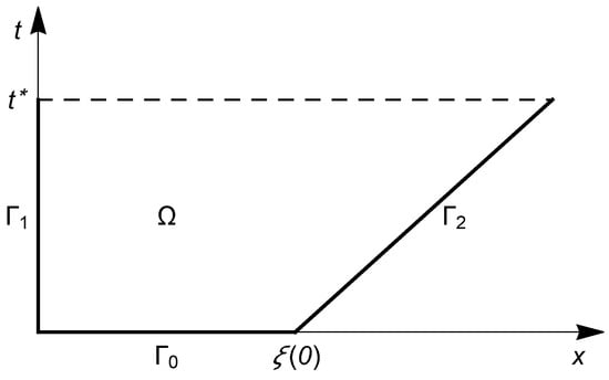
Figure 1.
The domain of the considered problem.
In the domain , we consider the following equation:
where is the order of the derivative of Caputo type, is the scaled (fractional) thermal diffusivity [], that is the thermal diffusivity [] multiplied by the scaling constant with the numerical value of one and unit [], and u, t and x refer to the temperature, time and spatial location respectively. On the boundaries and we set the following conditions:
where k is the thermal conductivity [], is scaled (fractional) latent heat of fusion per unit volume [], that is the latent heat of fusion per unit volume [] multiplied by the scaling constant with the numerical value of one and unit [], is the phase change temperature []. On the boundary we do not set any boundary condition as we are going to reconstruct it in the inverse problem.
The fractional derivative used in the above equations is of Caputo type. For this derivative is defined as follows [6]:
where is the gamma function.
In case of the direct Stefan problem we know all of the functions and parameters describing the initial and boundaries conditions, as well as the material physical parameters and we are looking for the temperature distribution and the position of the moving interface. In case of the inverse problem, in turn, we do not know a part of the input information, e.g., the function describing the boundary conditions, but we do know, however, something about the solution. When considering the Stefan inverse problem, this known information is more often than not, the temperature in the chosen points of the domain or the position of the moving interface. The inverse problems for which the position of moving interface is known are the so-called inverse design problems.
The presented inverse Stefan problem consists in finding a function u which describes the temperature distribution in domain and reconstruct functions and q describing the temperature and the heat flux on the boundary , which will satisfy Equations (4)–(7). We assume that all of the other functions and parameters are known.
3. Solution of the Problem
For solving the discussed problem, the homotopy analysis method will be used. This method was elaborated by the Chinese mathematician Shijun Liao and is designed for solving various kind of linear and nonlinear operator equations. For the first time the method was described in 1992 in its author PhD thesis [28] and has found an application in various fields since then. It allows us to solve the operator equation:
where N is operator (in particular it can be the nonlinear operator), whereas u is unknown function. First we define the homotopy operator as [29]:
where is an embedding parameter, is an auxiliary function, the convergence control parameter, an initial approximation of the solution of problem (8) and L an auxiliary linear operator.
Considering the equation , we get the so-called zero-order deformation equation:
For we have , from which we obtain . In turn, because for we get , then , where u is the sought solution of the Equation (8). This way the change of the parameter p from zero to one is corresponding to the change from the trivial problem to the original problem.
By expanding the into the Maclaurin series with regards to the parameter p and transforming it we get:
where
where is mth-order homotopy-derivative operator [29]:
If the series that occurs in the Formula (11) is convergent in the proper area, then for the we obtain the sought solution:
As the approximate solution we can choose the partial sum of the above series:
To find the exact or approximate solution of the discussed equation it is necessary to determine the function . For this we need to differentiate the left and right side of the Formula (10) m-times, with regards to the parameter p, then we divide the obtained result by and substitute obtaining the formula that is called the mth-order deformation equation ():
where
By the proper choice of the h parameter, which was introduced in the Formula (9), we can impact the region of convergence of the series (13) and its convergence rate [29,30,31]. This is why it is called the convergence control parameter [32,33,34]. One of the methods of choosing the value of this parameter is the so-called “optimization method” [29]. In this method the residue (deviation) function is defined for the considered equation and determined approximate solution :
The optimum value of the convergence control parameter is obtained by finding the argument for which the function reaches its minimum.
The effective region of the convergence control parameter is also defined as follows:
If we choose the value of the convergence control parameter different than the optimum but still from the effective region , the obtained series will also be convergent but the rate of the convergence will be lower. The version of the method including the described above selection of the optimum value of the convergence control parameter is called the basic optimal homotopy analysis method [29].
In order to speed up the computation, Liao [29] suggests to substitute the integral in the Formula (17) by its approximate value using the appropriate numerical integration method. In the examples demonstrated by him, the obtained values of the convergence control parameter did not differ much from the values obtained by the application of the Formula (17).
In the discussed problem the N operator has the form:
However, as the linear operator L we can choose the operator of form:
Assuming that the series is convergent then for the derivative of a Caputo type we get:
By using it we obtain:
for and where for . Likewise we get:
Taking into account the L operator we obtain the set of partial differential equations that allow us to determine the functions . For we have:
and for :
To make the solution unambiguous, we need to supplement the above partial differential equations with additional conditions. For this we will use the conditions () and (). First equation we supplement with the conditions of form:
For the rest of the equations (), on the other hand, we set the conditions of form:
The above conditions provide us with the fact that any approximate solution constructed as the partial sum of the series (13) will meet the specified boundary conditions. As the initial approximation we can take the function that determines the initial condition:
Therefore, the problem was reduced to solving a series of partial differential Equations (26) and (27), with the conditions (28) and (29) and (30) and (31) respectively. The obtained equations are easier to solve than the initial problem. By knowing the function u or its approximation , we can easily determine the missing boundary conditions:
or their approximations:
It can be shown that the sum of the constructed series is a solution of the discussed equation.
Theorem 1.
The next theorem gives the sufficient condition for the convergence of the series constructed in the method.
Theorem 2.
Let the functions , be the solutions of the Equations (26) and (27) with the conditions (28) and (29) and (30) and (31) respectively. Then if the parameter h is selected in such a way that there exist such constants and that for each the inequality
is satisfied in the domain Ω, then the series is uniformly convergent in Ω.
The last theorem gives the approximate solution error estimation, which we obtain using the partial sum of the series.
Theorem 3.
If assumptions of Theorem 2 are satisfied and additionally and , then the estimation of error of the approximate solution is described by the following formula:
where is determined by the Equation (14).
The proofs for all of the above theorems are similar to those for the classic Stefan inverse problem and may be found in the paper [27].
4. Example
We will now present the method outlined in the previous chapter using an example. We will consider the problem for which under discussion we take the following data: , , , , , , , . Let us mention that all of the calculations presented here were carried out with the aid of Mathematica software [35].
Assuming that in the first step, we get:
and
The optimal value of the convergence control parameter equals to . Figure 2 displays the graph of logarithm of the squared residual for . This way for this value of h parameter we obtain the following approximate solutions:
and
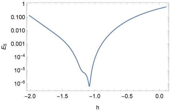
Figure 2.
Logarithm of the squared residual .
Figure 3 displays the reconstructed boundary conditions, which are the temperature distribution and the heat flux on the boundary . The obtained approximate temperature distribution for the whole area whereas is presented in the Figure 4. The next Figure 5, however, presents the convergence of the sequence of the partial sums which are the consecutive approximate solutions. In the picture the graphs of functions and are presented using a logarithmic scale for . The functions and determine the approximate temperature distribution and the heat flux on the boundary , and are defined by Formulas (35) and (36) respectively. The logarithmic scale was used because all of those functions take very small values. At points where a peak down appears on the graph the corresponding function for which the absolute value is taken changes its sign. This way the absolute value equals to zero and its logarithm tends to minus infinity. Graphs of the and functions without a logarithmic scale are presented in Figure 6. Figure 5 shows as well that for the obtained approximate solutions the inequality (37) holds. We may assume that the next approximations will behave the same way. This way according to Theorem 2 the series forming the approximate solution is convergent, so its sum is the sought solution (see Theorem 1).
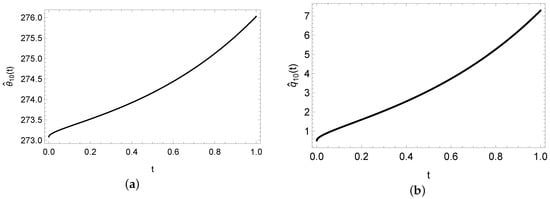
Figure 3.
The reconstructed boundary conditions: (a) temperature distribution , (b) heat flux .
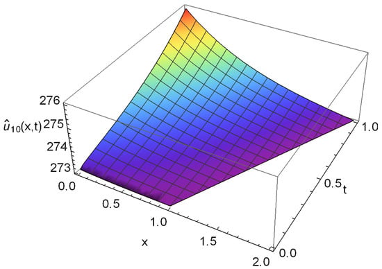
Figure 4.
The reconstructed temperature distribution in the area .
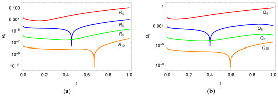
Figure 5.
The presentation of convergence (on a logarithmic scale): (a) temperature distribution, where , (b) heat flux, where .
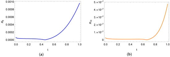
Figure 6.
Functions without a logarithmic scale: (a) function , (b) function .
In the considered inverse problem, the information compensating for the lack of part of the input data is the known position of the moving interface. Therefore, in the example the stability of the procedure was also examined by terms of the errors of this position determination. The location of the moving interface was given with the random 1%, 2%, 5% and 10% errors. The relative errors of the boundary conditions reconstruction on the boundary and the temperature distribution in the area determined by the norm are displayed in the Table 1. The relative errors were calculated for the shifted temperature (). In this case they achieve the greatest values then. For the output temperature the relative errors do not exceed the % (for the greatest disturbance). In case of the heat flux, the shift does not affect the relative error. In the case when the input data gets disturbed by the and errors, the errors of reconstruction are on a similar level. Only for the bigger disturbances of the input data the errors of reconstruction increase by about relative to the value of the input data disturbance. These errors are not yet very drastic, especially if looking at the course of the reconstructed curves representing the boundary conditions (see Figure 7). As can be seen, the shape of the proper curve has been maintained for each case. The graphs of the absolute errors of the boundary conditions reconstruction for various disturbances of the input data are displayed in the Figure 8. The Figure 9 just like before presents the convergence of the approximate solutions in case of the input data disturbed by the error.

Table 1.
The relative errors of reconstruction the boundary conditions and temperature distribution for the disturbed input data.
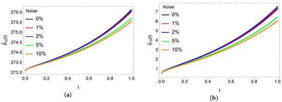
Figure 7.
The reconstructed boundary conditions for the various noise of input data: (a) temperature distribution , (b) heat flux q.
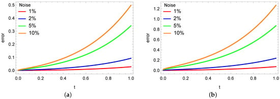
Figure 8.
The absolute errors of the boundary conditions reconstruction for the various noise of the input data: (a) temperature distribution , (b) heat flux q.
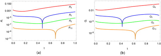
Figure 9.
The presentation of convergence for the input data disturbed by the error: (a) temperature distribution, where , (b) heat flux, where .
The Figure 10 presents the reconstructed boundary conditions for the different values of the order of the Caputo derivative . For this method converges quickly. The obtained solutions get bigger values with increasing value of the parameter. On the other hand, for the improper integrals that occur during the calculations do not converge. Thus, the method cannot be used in this case.
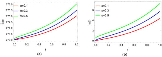
Figure 10.
The reconstructed boundary conditions for different values of the order of the fractional derivative: (a) temperature distribution , (b) heat flux q.
5. Conclusions
We use the homotopy analysis method to solve the one-phase fractional inverse Stefan problem. The mathematical model considered in the paper consists of a differential equation with a Caputo fractional derivative and the conditions on the boundaries of the considered domain, with the temperature distribution and heat flux unknown on one of the boundaries. In order to find these unknown functions, in accordance with the homotopy analysis method, an appropriate series is constructed which, if it converges, is the solution of the considered equation. We present theorems concerning the series convergence as well as the estimation of the error of the approximate solution. We also present a numerical example illustrating the application of the described method, its convergence and stability to the disturbances of the input data. As can be seen in the figures and the table presented in Section 4, the method converges quickly and the errors of the approximate solution are relatively small, especially for the input data disturbed by the 1% or 2% error. An important advantage of the method is the fact that the solution is obtained in the form of a continuous function and the considered domain does not need to be discretized. In the future, we plan to apply the method to two-phase and multidimensional problems, as well as to models with other types of fractional order derivative.
Author Contributions
Conceptualization, D.S.; Methodology, D.S.; Software, D.S., R.B. and M.S.; Validation, D.S., A.C. and M.S.; Formal Analysis, D.S., R.B., A.C. and M.S.; Investigation, D.S., R.B. and A.C.; Writing—Original Draft Preparation, D.S. and A.C.; Writing—Review and Editing, D.S., R.B., A.C. and M.S.; Visualization, D.S., R.B. and M.S.; Funding Acquisition, D.S. All authors have read and agreed to the published version of the manuscript.
Funding
This research received no external funding.
Acknowledgments
Publication supported within the framework of grants in the area of scientific research and developmental works founded by Rector of the Silesian University of Technology, 09/010/RGJ19/0041.
Conflicts of Interest
The authors declare no conflict of interest.
Nomenclature
| a | scaled (fractional) thermal diffusivity [] |
| thermal diffusivity [] | |
| homotopy-derivative operator | |
| E | residue function |
| homotopy operator | |
| h | convergence control parameter |
| k | thermal conductivity [] |
| L | linear operator |
| N | operator (linear or nonlinear) |
| p | embedding parameter |
| q | heat flux [] |
| Q | auxiliary function [] |
| effective region | |
| R | auxiliary function [] |
| t | time [] |
| end of time interval [] | |
| u | temperature [] |
| phase change temperature [] | |
| initial approximation [] | |
| scaling constant [] | |
| x | spatial variable [] |
| Greek symbols | |
| order of the Caputo derivative | |
| boundary of the region | |
| gamma function | |
| temperature [] | |
| scaled (fractional) latent heat of fusion per unit volume [] | |
| latent heat of fusion per unit volume [] | |
| position of the moving interface [] | |
| auxiliary function [] | |
| initial temperature [] | |
| auxiliary parameter | |
| region | |
| Superscripts | |
| refers to approximations | |
| Subscripts | |
| n | order of the approximation |
References
- Carpinteri, A.; Mainardi, F. Fractal and Fractional Calculus in Continuum Mechanics; Springer: New York, NY, USA, 1997. [Google Scholar]
- Hilfer, R. Applications of Fractional Calculus in Physics; World Scientific: Singapore, 2000. [Google Scholar]
- Kosztołowicz, T. Application of the Differential Equations with Fractional Derivatives for Describing the Subdiffusion; Jan Kochanowski University Press: Kielce, Poland, 2008. [Google Scholar]
- Leszczyński, J. An Introduction to Fractional Mechanics; The Publishing Office of Czȩstochowa University of Technology: Czȩstochowa, Poland, 2011. [Google Scholar]
- Mitkowski, W.; Kacprzyk, J.; Baranowski, J. Advances in the Theory and Applications of Non-Integer Order Systems; Springer Inter. Publ.: Cham, Switzerland, 2013. [Google Scholar]
- Podlubny, I. Fractional Differential Equations; Academic Press: San Diego, CA, USA, 1999. [Google Scholar]
- Diethelm, K. The Analysis of Fractional Differential Equations; Springer: Berlin, Germany, 2010. [Google Scholar]
- Obra̧czka, A.; Mitkowski, W. The comparison of parameter identification methods for fractional partial differential equation. Solid State Phenom. 2014, 210, 265–270. [Google Scholar] [CrossRef]
- Szymanek, E.; Blaszczyk, T.; Hall, M.; Dehdezi, P.; Leszczynski, J. Modelling and analysis of heat transfer through 1D complex granular system. Granul. Matter 2014, 16, 687–694. [Google Scholar] [CrossRef]
- Zhuang, Q.; Yu, B.; Jiang, X. An inverse problem of parameter estimation for time-fractional heat conduction in a composite medium using carbon–carbon experimental data. Physica B 2015, 456, 9–15. [Google Scholar] [CrossRef]
- Voller, V. Anomalous heat transfer: Examples, fundamentals, and fractional calculus models. Adv. Heat Transf. 2018, 50, 333–380. [Google Scholar]
- Sierociuk, D.; Dzieliński, A.; Sarwas, G.; Petras, I.; Podlubny, I.; Skovranek, T. Modelling heat transfer in heterogeneous media using fractional calculus. Philos. Trans. R. Soc. A 2013, 371, 20120146. [Google Scholar] [CrossRef] [PubMed]
- Brociek, R.; Słota, D.; Król, M.; Matula, G.; Kwaśny, W. Comparison of mathematical models with fractional derivative for the heat conduction inverse problem based on the measurements of temperature in porous aluminum. Int. J. Heat Mass Transf. 2019, 143, 118440. [Google Scholar] [CrossRef]
- Rajeev, M.S.; Kushwaha, A.K. An approximate solution to a moving boundary problem with space-time fractional derivative in fluvio-deltaic sedimentation process. Ain Shames Eng. J. 2013, 4, 889–895. [Google Scholar] [CrossRef][Green Version]
- Kushwaha, M.S. Homotopy perturbation method for a limit case Stefan problem governed by fractional diffusion equation. Appl. Math. Model. 2013, 37, 3589–3599. [Google Scholar] [CrossRef]
- Liu, J.; Xu, M. An exact solution to the moving boundary problem with fractional anomalous diffusion in drug release devices. Z. Angew. Math. Mech. 2004, 84, 22–28. [Google Scholar] [CrossRef]
- Yin, C.; Li, X. Anomalous diffusion of drug release fromslabmatrix: Fractional diffusion models. Int. J. Pharm. 2011, 418, 78–87. [Google Scholar] [CrossRef]
- Voller, V. Computations of anomalous phase change. Int. J. Numer. Methods Heat Fluid Flow 2016, 26, 624–638. [Google Scholar] [CrossRef]
- Liu, J.; Xu, M. Some exact solutions to Stefan problems with fractional differential equations. J. Math. Anal. Appl. 2009, 351, 536–542. [Google Scholar] [CrossRef]
- Roscani, S.; Marcus, E. A new equivalence of Stefan’s problems for the time fractional diffusion equation. Fract. Calc. Appl. Anal. 2014, 17, 371–381. [Google Scholar] [CrossRef][Green Version]
- Roscani, S.; Tarzia, D. Explicit solution for a two-phase fractional Stefan problem with a heat flux condition at the fixed face. Comp. Appl. Math. 2018, 37, 4757–4771. [Google Scholar] [CrossRef]
- Błasik, M.; Klimek, M. Numerical solution of the one phase 1D fractional Stefan problem using the front fixing method. Math. Methods Appl. Sci. 2014, 38, 3214–3228. [Google Scholar] [CrossRef]
- Błasik, M. Numerical scheme for one-phase 1D fractional Stefan problem using the similarity variable technique. J. Appl. Math. Comput. Mech. 2014, 13, 13–21. [Google Scholar] [CrossRef][Green Version]
- Błasik, M. A numerical method for the solution of the two-phase fractional Lamé-Clapeyron-Stefan problem. arXiv 2018, arXiv:1810.12072. [Google Scholar]
- Kushwaha, M.S. Comparison between Adomian decomposition method and optimal homotopy asymptotic method for a two moving boundaries problem. Differ. Equ. Dyn. Syst. 2020, 28, 431–446. [Google Scholar] [CrossRef]
- Hetmaniok, E.; Słota, D.; Wituła, R.; Zielonka, A. Solution of the One-Phase Inverse Stefan Problem by Using the Homotopy Analysis Method. Appl. Math. Model. 2015, 39, 6793–6805. [Google Scholar] [CrossRef]
- Hetmaniok, E.; Słota, D.; Wituła, R.; Zielonka, A. An Analytical Method for Solving the Two-Phase Inverse Stefan Problem. Bull. Pol. Acad. Sci. Tech. Sci. 2015, 63, 583–590. [Google Scholar] [CrossRef][Green Version]
- Liao, S. On the Proposed Homotopy Analysis Techniques for Nonlinear Problems and Its Application. Ph.D. Thesis, Shanghai Jiao Tong University, Shanghai, China, 1992. [Google Scholar]
- Liao, S. Homotopy Analysis Method in Nonlinear Differential Equations; Springer: Berlin, Germany; Higher Education Press: Beijing, China, 2012. [Google Scholar]
- Odibat, Z. A study on the convergence of homotopy analysis method. Appl. Math. Comput. 2010, 217, 782–789. [Google Scholar] [CrossRef]
- Turkyilmazoglu, M. Convergence of the homotopy analysis method. arXiv 2010, arXiv:1006.4460v1. [Google Scholar]
- Liao, S. Notes on the homotopy analysis method: Some definitions and theorems. Commun. Nonlinear Sci. Numer. Simul. 2009, 14, 983–997. [Google Scholar] [CrossRef]
- Van Gorder, R.; Vajravelu, K. On the selection of auxiliary functions, operators, and convergence control parameters in the application of the homotopy analysis method to nonlinear differential equations: A general approach. Commun. Nonlinear Sci. Numer. Simul. 2009, 14, 4078–4089. [Google Scholar] [CrossRef]
- Russo, M.; Van Gorder, R. Control of error in the homotopy analysis of nonlinear Klein-Gordon initial value problems. Appl. Math. Comput. 2013, 219, 6494–6509. [Google Scholar] [CrossRef]
- Wolfram, S. An Elementary Introduction to the Wolfram Language; Wolfram Media: Champaign, IL, USA, 2017. [Google Scholar]
Publisher’s Note: MDPI stays neutral with regard to jurisdictional claims in published maps and institutional affiliations. |
© 2020 by the authors. Licensee MDPI, Basel, Switzerland. This article is an open access article distributed under the terms and conditions of the Creative Commons Attribution (CC BY) license (http://creativecommons.org/licenses/by/4.0/).