Longitudinal Modelling and Control of In-Wheel-Motor Electric Vehicles as Multi-Agent Systems

Abstract

This paper deals with longitudinal motion control of electric vehicles (EVs) driven by in-wheel-motors (IWMs). It shows that the IWM-EV is fundamentally a multi-agent system with physical interaction. Three ways to model the IWM-EV are proposed, and each is applicable to certain control objectives. Firstly, a nonlinear model with hierarchical structure is established, and it can be used for passivity-based motion control. Secondly, a linearized model with rank-1 interconnection matrix is presented for stability analysis. Thirdly, a time-varying state-space model is proposed for optimal control using linear quadratic regulator (LQR). The proposed modellings contribute the new understanding of IWM-EV dynamics from the view point of multi-agent-system theory. By choosing the suitable control theory for each model, the complexity level of system design is maintained constant, no matter what the number of IWMs installed to the vehicle body. The effectiveness of three models and their design approaches are discussed by several examples with Matlab/Carsim co-simulator.

1. Introduction

In-wheel-motors (IWMs) have been shown a novel actuator for motion control system of electric vehicles (EVs) [1]. A remarkable merit of IWM-EV is the ability to precisely generate the driving/braking torques with fast response at individual wheels. Based on this merit, various motion control strategies have been developed in three dimensions. Through literature review, motion control of electric vehicle can be categorized by several sub-fields as follows:

(i) Lateral motion control: By differentiating the torques distributed to the left-side and right-side wheels, a yaw-moment is generated about the vertical axis of the vehicle body. This allows us to stabilize the lateral motion of the vehicle via direct-yaw-moment control [2]. Some important issues of this sub-field are sides-slip angle estimation [2,3], side-slip angle and yaw-rate control [4], and the integration of direct-yaw-moment control with active-steering control [5].

(ii) Roll motion control: By allocating the motor torques suitably, it is also possible to generate the roll moment about the longitudinal axis. This moment can be used to control the roll angle and roll rate for improving the comfort of the driver [6].

(iii) Pitch motion control: By distributing the different torques to the front-wheels and rear-wheels, a pitch moment is generated about the lateral axis. This moment could be used to improve the pitch motion, as presented in [7,8,9].

(iv) Longitudinal motion control: This is the objective of this paper. Longitudinal motion control (LMC) of EV can be summarized by three main groups in

Table 1. Review of longitudinal motion control methods for EVs.

Group	Strategy	Consideration of Physical Interaction (YES/NO)	References
(I) Slip ratio control	Sliding mode control	NO	[10,11,12,13]
	PI control by linearizing the slip dynamics	NO	[14,15,16]
	Optimal control by hierarchical LQR	YES	[17]
(II) Anti-slip control	Zero-slip-model following control	NO	[18,19]
	Maximum transmissible torque estimation	NO	[20,21]
	Direct wheel velocity control	NO	[22]
(III) Driving force control	Direct driving force control	NO	[23]
	Driving force control based on wheel velocity control and virtual variable control	NO	[24,25,26]

, namely, (I) slip ratio control [10,11,12,13,14,15,16,17], (II) anti-slip control [18,19,20,21,22], and (III) driving force control [23,24,25,26].

In recent years, an uptrend has been observed in the number of IWM actuators installed to the vehicle body. For instance, France Army developed the armored vehicle DPE 6 × 6 which is driven by six independent motors [27]. In Japan, Keio University introduced the prototype of KAZ-EV with eight IWMs [28]. Thanks to the development of wireless IWM technology [29], powerful EVs driven by more than ten IWMs might be soon realized. With respect to this uptrend, IWM-EV should be treated as a multi-agent system in which each local agent is a locally controlled wheel. The local agent cooperates with each other through the vehicle body to generate the global motion of the vehicle body as well as its local motion.

From the above discussion, LMC of IWM-EVs becomes an actual challenge. Fortunately, it is possible to apply the state-of-the-art of multi-agent system theories. Among them, the global (global/local) framework proposed by Hara group has been shown an effective way to model, analyze, and design multi-agent dynamical systems [30]. Several successful examples of glocal control are gene-regulatory network [31], platoon car [32,33], and manufacturing systems [34]. We recently developed a scheme in the glocal theory family, namely, hierarchical linear quadratic regulator (H-LQR), and applied it to optimal control of slip ratio for IWM-EVs in the acceleration mode [17]. The key of H-LQR is to utilize some special features in the structure of the multi-agent system to reduce the design cost. From the view point of glocal control framework, two critical issues still remain in the research field of LMC for IWM-EVs.

Firstly, almost the previous studies (including the works mentioned in Table 1) neglected the physical interaction between the wheel dynamics. For instance, in [22], Suzuki et al. introduced an anti-slip control by directly controlling the wheel velocity. The wheel velocity controller C_w(s) is merely designed by stable pole-placement to the closed-loop of C_w(s) and P_w(s) which represent the local wheel dynamics. In [25], Maeda et al. proposed the driving force control system for the four-IWM-EV. However, the system is just the combination of four decoupled wheel-velocity-based force control loops. In [11], Nam et al. independently design for each wheel a sliding-mode slip ratio controller. However, the design is based on the single wheel dynamics model without any relevant to the others. Actually, the physical interaction exists as the wheels are installed to the same car body. As clarified by a glocal control tool, namely “generalized frequency variable theory” [35], and its application to EV [36], neglecting physical interaction might reduce the system performance. Even if each wheel’s control loop is locally stable, this does not automatically guarantee the stability of the IWM-EV system as a whole. Therefore, it is essential to model the IWM-EV as an interconnected system of multi-agents to properly design the LMC.

Secondly, following the uptrend in the number of IWM actuators, analyzing and designing the LMC systems become more and more complex. Increasing the actuator numbers means increasing the order of the system, and hence the implementation effort and the computational cost. Even if we can model the LCM system with physical interactions, how should we select the suitable control theory to reduce the burden of design and analysis?

To tackle the aforementioned issues, proper modelling is necessary. In other words, the model should capture the essential characteristics of the plant in the physical world. Looking at the literature of EV-related-study, this philosophy of modelling has been pointed out by several recent works on battery management and control [37,38,39,40]. For instance, in [37], a predictive control algorithm of charging process was proposed by utilizing a thermoelectric model which accurately captures the battery dynamics. Recently, a Gaussian process regression models have been used to address the aging phenomenon of batteries in [39].

To provide the proper models for LMC of IWM-EVs, this paper is based on the glocal framework. The strategy of this paper is described in Figure 1 which includes three spaces. In the physical world, the motion of the IWM-EV is governed by the physical equations. From the view point of multi-agent systems, the physical model is mapped to the control world by three design models (DMs). Each DM is suitable for a certain objective of longitudinal motion control. Moreover, each DMs is associated with a control theory developed in the glocal framework, such that the complexity of system design and analysis is independent of the number of IWM actuators. Three proposed DMs are briefly explained as follows.

DM-1 (nonlinear model with hierarchical structure): DM-1 consists of the vehicle body dynamics V in the upper-layer, and a bunch of local wheel dynamics {W_i} in the lower-layer. The two layers interconnect with each other through the aggregation and distribution channels. This expression is quite useful for designing LMC by passivity theory [41]. The advantage of using DM-1 and the passivity theory is that we can design the control system with less mathematical effort and prove the system stability rigorously. In this paper, a passivity based anti-slip control system is proposed to demonstrate the effectiveness of DM-1.

DM-2 (linearized model with rank-1 interconnection matrix): DM-2 is established by linearizing the nonlinear physical equations of IWM-EV about a given operating point, and it is useful for stability analysis. As an example, DM-2 is applied to wheel velocity control with work-load minimization. Thanks to the rank-1 interconnection matrix and the generalized frequency variable (GFV) theory [35], the complexity of stability analysis is considerably reduced. The stability analysis can be performed by a limited set of inequalities established from the GFV transfer function and the eigenvalues of the interconnection matrix. DM-2 and the GFV makes up the useful tools to design and analyze any existing LMC methods.

DM-3 (time-varying state-space model): DM-3 is proposed for capturing the slip ratio dynamics and driving force dynamics of IWM-EV in the state space expression. Hence, this model can be used for applying the optimal control strategies and updating the optimal control gains in real-time operation. In our recent study [17], DM-3 was established in the acceleration mode. To complete the state space modelling for LMC, this paper investigates the DM-3 in the deceleration mode. We theoretically show that global optimality can be achieved by a hierarchical LQR (H-LQR) algorithm in which we only need to solve the local Riccati equation. Applying the proposed H-LQR, the computational cost is effectively reduced.

The remainder of this paper is organized as follows. Section 2 presents the physical equations that describing the longitudinal motion of IWM-EV. To clarify the motivation of this paper, Section 3 discusses the disadvantages of the traditional LMC methods by numerical simulations. Then, DM-1, DM-2, and DM-3 are investigated in Section 4, Section 5 and Section 6, respectively. Each of the proposed DMs is established under reasonable assumptions, following by a motion control example. Section 7 presents the simulation results of the motion control examples in Section 4, Section 5 and Section 6. The simulations were conducted using a Matlab/Casim co-simulator which is based on an experimental electric vehicle developed by our research group. Finally, the concluding remarks are given in Section 8.

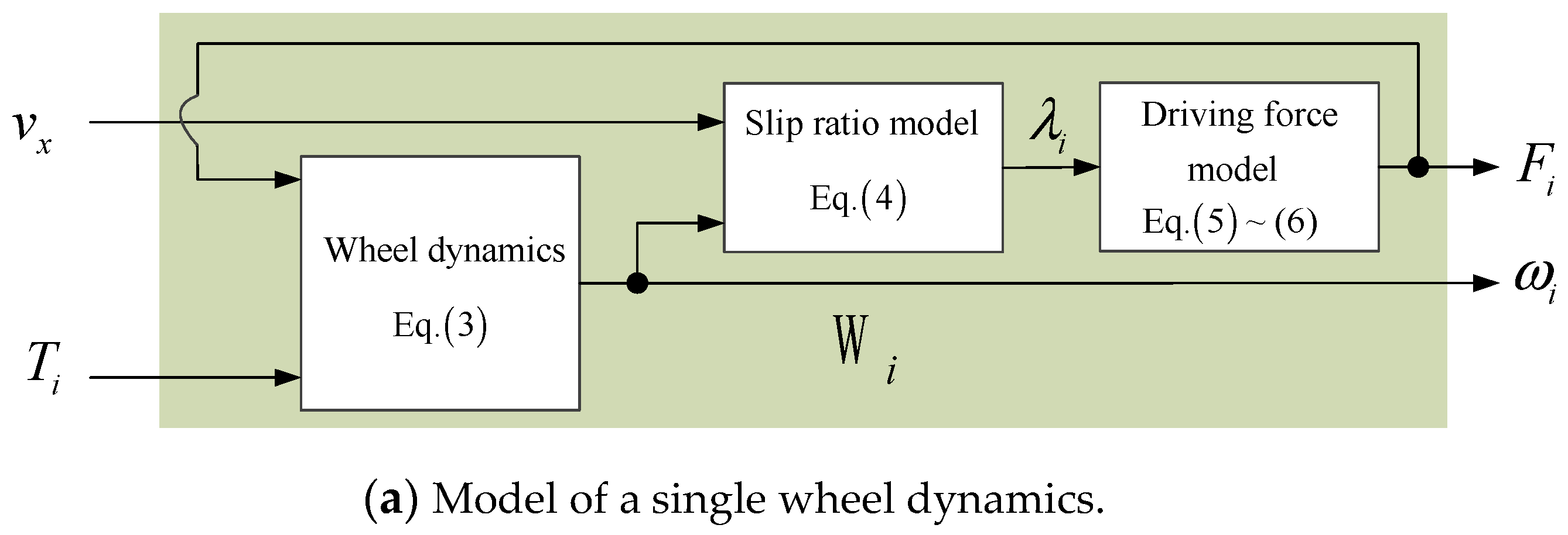
2. Longitudinal Dynamics of Vehicle

This paper examines the longitudinal motion of IWM-EV illustrated in Figure 2 of which the number N of IWMs is an even number. Let m be the vehicle mass. Under the assumption that the wheels are homogeneous, J_w and r are the inertia and radius of the wheel, respectively. T_i, F_i, and Z_i are the motor torque, the driving force, and the vertical force acting at the ith wheel, respectively. The local motion of the ith wheel is represented by the rotational velocity ω_i. The global motion of the vehicle body is represented by the longitudinal velocity v_x. F_air is the air resistance acting on the vehicle body. The total influence of gravity and rolling resistance is represented by F_ξ.

The motion of the vehicle body is given by

$$m{\dot{v}}_x={\displaystyle \sum _{i=1}^N{F}_i}-F_{air}-F_{\xi }.$$

(1)

Neglecting the wind velocity, the air resistance is expressed as

$$F_{air}=\rho v_x\left|v_x\right|,$$

(2)

where the coefficient ρ is calculated from the density of air, the cross-sectional area of the vehicle in the air, and the drag coefficient which depends on the shape of the vehicle [42].

The rotational motion of the ith wheel is given as

$$J_w{\dot{\omega }}_i=T_i-r{F}_i.$$

(3)

Let ε be a small number to avoid division-by-zero, the slip ratio of the ith wheel is defined as

$${\lambda }_i=\frac{r{\omega }_i-v_x}{\max \left\{r{\omega }_i,v_x,\epsilon \right\}}.$$

(4)

The nonlinear relationship between the driving force and the slip ratio can be described by several empirical functions. The most popular one is the magic formula proposed by Pacejka [43]. This formula is given by

$$f_i({\lambda }_i)=A_i\sin \left\{B_i{\tan }^{-1}\left[C_i{\lambda }_i-D_i\left(C_i{\lambda }_i-{\tan }^{-1}\left(C_i{\lambda }_i\right)\right)\right]\right\},$$

(5)

where A_i, B_i, C_i, and D_i are the shape factors, with A_i = μ_iZ_i where μ_i is the friction coefficient. Note that the friction coefficient and the shape factors are all identifiable from experimental data. Now, the driving force is expressed as

$$F_i({\lambda }_i)=\{\begin{array}{c}{f}_i({\lambda }_i)\mathrm{if}{\lambda }_i\ge 0\\ -f_i(-{\lambda }_i)\mathrm{if}{\lambda }_i<0\end{array}.$$

(6)

The typical curve of the driving force is shown in Figure 3. The driving force gradually increases as the slip ratio increases from 0 to an optimal value λ* which depends on the road condition. Since the slip ratio exceeds λ*, the driving force is decreased to a minimum value as the slip ratio approach to 1. Investigating the magic formula, we suggest the following practical remark.

Remark 1:

The inequalityλ_if_i(λ_i) ≥ 0 holds for any value of slip ratioλ_iin (−1, 1).

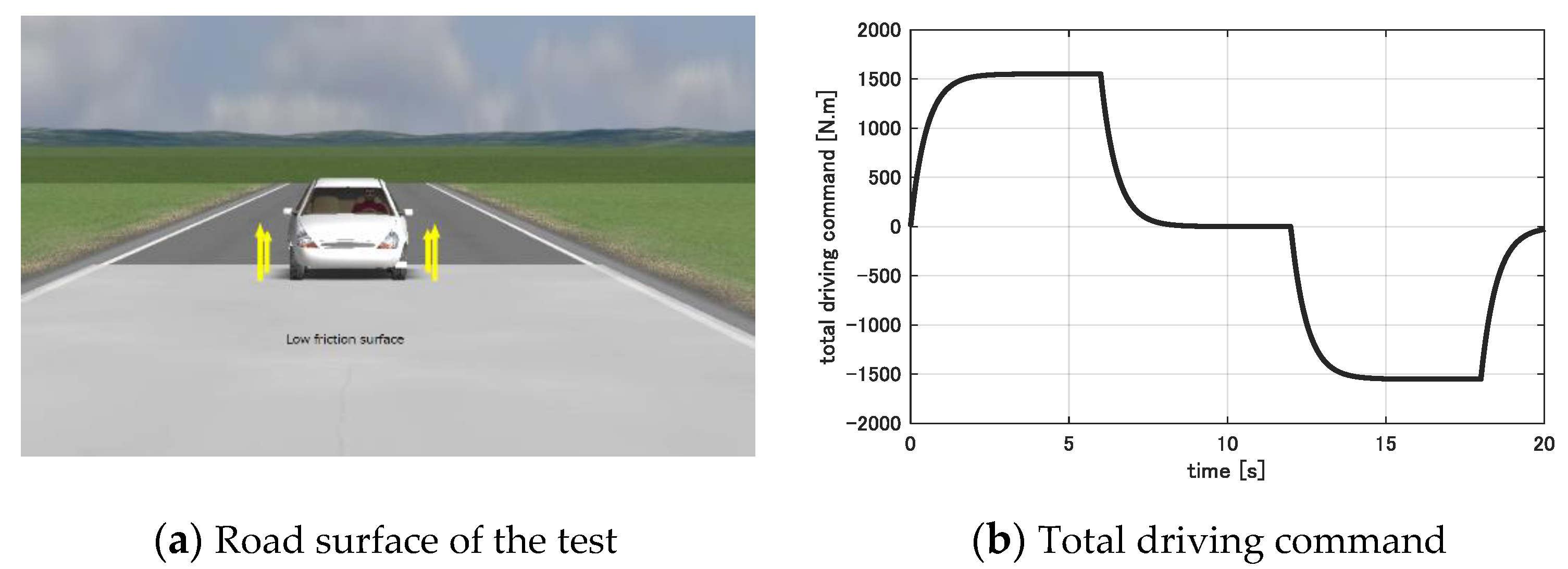
3. Motivating Example

In our recent study [17], we examined the slip ratio control method proposed in [14] by both theoretical discussion and numerical simulations. According to [14], it is possible to linearize the dynamics from the motor torque T_i to the slip ratio λ_i. Then, a PI controller can be designed by placing the stable poles to the local subsystem. However, the performance of the overall system should be determined by both local subsystem’s transfer function and a matrix that representing physical interaction [35]. Due to the change of operating points, the poles of the overall system might move towards the imaginary axis with increasing imaginary parts. This phenomenon might degrade the system performance by several scenarios. For instance, oscillated phenomena can be observed when the vehicle runs at high velocity. In addition, the load transfer can introduce large gap between the slip ratios of the front-wheels and rear-wheels. Moreover, the traditional slip ratio control system is highly sensitive to the non-flatness of the road surfaces.

This paper neglects to re-simulate the aforementioned slip ratio control method. Instead, we examine another LMC method, namely, anti-slip control by wheel velocity control [22]. To this end, this paper utilizes Carsim—a standard software for simulating the vehicle dynamics [44]. By using Carsim, it is convenient to perform the control algorithms under different environmental conditions, including the dangerous conditions. The simulation model is built based on the four-wheel experimental electric vehicle developed from the Mitsubishi’s i-MiEV prototype. It was an outcome of our research project KC.03.08/11-15 supported by the Ministry of Science and Technology of Vietnam. The main specification of the vehicle is summarized in Appendix A.

To establish the simulation model, we modify the parameters of a hatchback car provided in the Library of Carsim. Since the Carsim only provide the vehicle of gasoline type, we constructed the electrical drive system in Matlab/Simulink. The electrical drive system consists of the battery model, the inverter models, the in-wheel-motor models of interior permanent magnet type, together with the inverter control units and motor control units. To resemble the behavior of the actual drive system, the inverter model imitates the electrical circuit of the experimental inverter. The output torques of the drive system model in Matlab/Simulink are sent to Carsim through the imports namely IMP_MYUSM_*. The notation * represents the IWM position (L1, L2, R1, and R2, where L denote “left” and R denotes “right”).

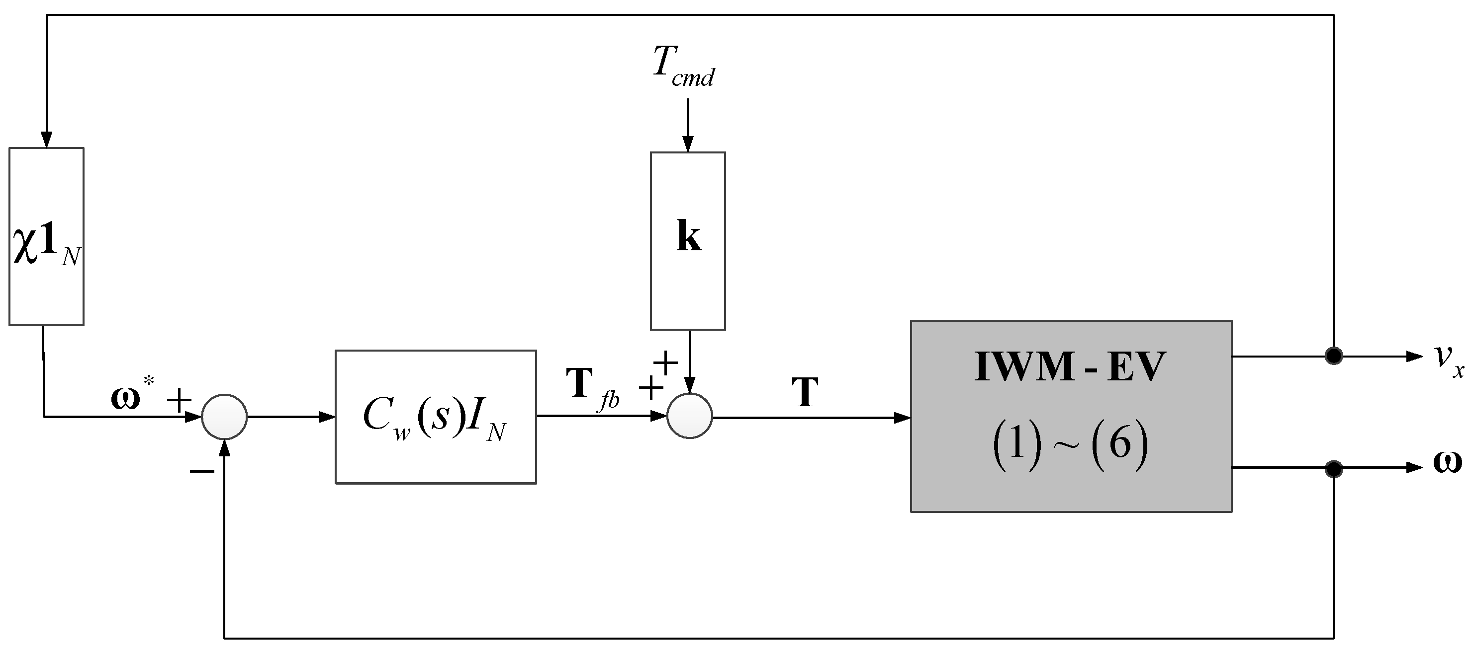
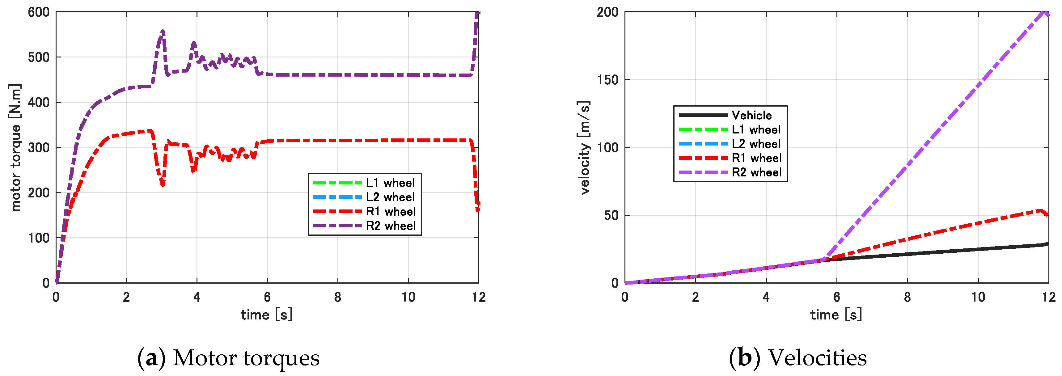
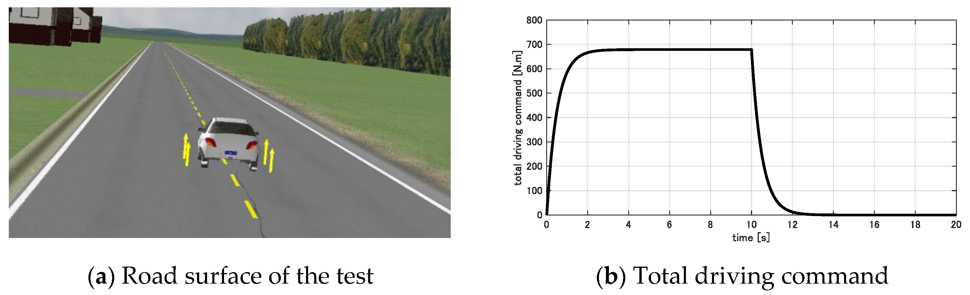
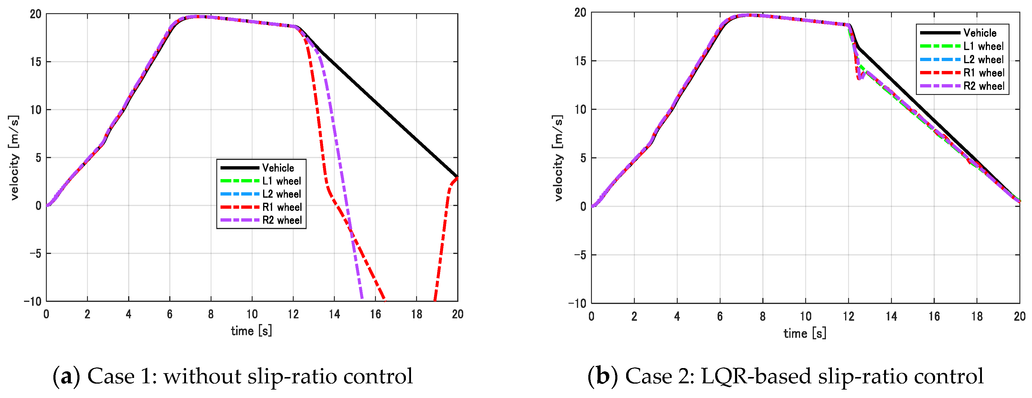
3.1. Anti-Slip Control Based on Wheel Velocity Control

Following the idea of the original work [22], we generalize the block diagram of the control system as in Figure 4. Here, 1_N is the all-one column-vector of size N, and T = [T₁ … T_N]^T, ω = [ω₁ … ω_N]^T. The scalar signal T_cmd is the driving command given by the driver or the upper motion control layer. In addition, vector k = [k₁ … k_N]^T is to distribute the driving command to the local wheel. The distribution ratio k_i are commonly selected such that 0 < k_i < 1 and k₁ + k₂ + … + k_N = 1. We assume that the vehicle operates on the acceleration mode when $r{\omega }_i>v_x$, and let ${\lambda }^{\ast }$ be the desired slip ratio. From (4), the reference velocity can be calculated from the wheel velocity v_x via the gain

$$\chi =\frac{1}{r\left(1-{\lambda }^{\ast }\right)}.$$

(7)

Each wheel is provided a velocity controller C_w(s). Let P_w(s) = 1/(J_ws) be transfer function that characterizes the local dynamics of the wheel. To design C_w(s), the traditional way is to assign the stable poles to the closed loop transfer function

$$P_{cl}(s)=\frac{P_w(s)C_w(s)}{1+P_w(s)C_w(s)}.$$

(8)

For instance, let ${\kappa }_1$ and ${\kappa }_2$ be the stable poles of P_cl(s), C_w(s) becomes a PI controller with the P gain and I gain calculated as

$$C_w(s)=\frac{K_{p}s+K_i}{s},K_p=-J_w\left({\kappa }_1+{\kappa }_2\right),K_i=J_w{\kappa }_1{\kappa }_2.$$

(9)

3.2. Simulation and Discussion

To evaluate the above design strategy, a test is conducted as follows. A constant driving command T_cmd is equally distributed to four wheels such that the EV accelerates from the initial position on the high friction surface (μ = 0.8). It enters the low friction surface (μ = 0.2) at about 4 s. Two test cases are performed, and their results are summarized in Figure 5.

Case A: Two stable poles of P_cl(s) are placed at ${\kappa }_{1,2}=-10\pm 2j$ (Figure 5a). The wheel velocities are maintained closed to the vehicle velocity. This means the anti-slip function is successfully attained in this case.

Case B: Two stable poles of P_cl(s) are placed at ${\kappa }_{1,2}=-100\pm 0j$ (Figure 5b). The overall system becomes unstable when the vehicle operates on the low-friction surface.

The simulation results in this sub-section suggest that local stabilization does not guarantee global stability of the control system. By using only the local wheel dynamics to design the controller, we cannot explain such performance of the vehicle in Case B. Therefore, it is necessary to model and design the motion control system of IWM-EV as a whole. Three models that effectively capture the physical interaction will be presented in the following three sections.

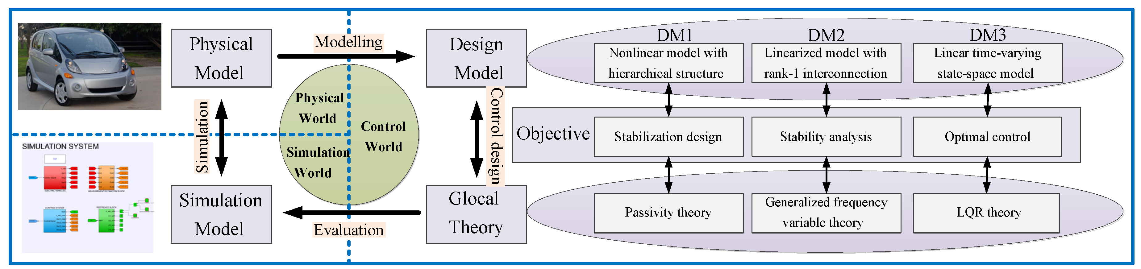
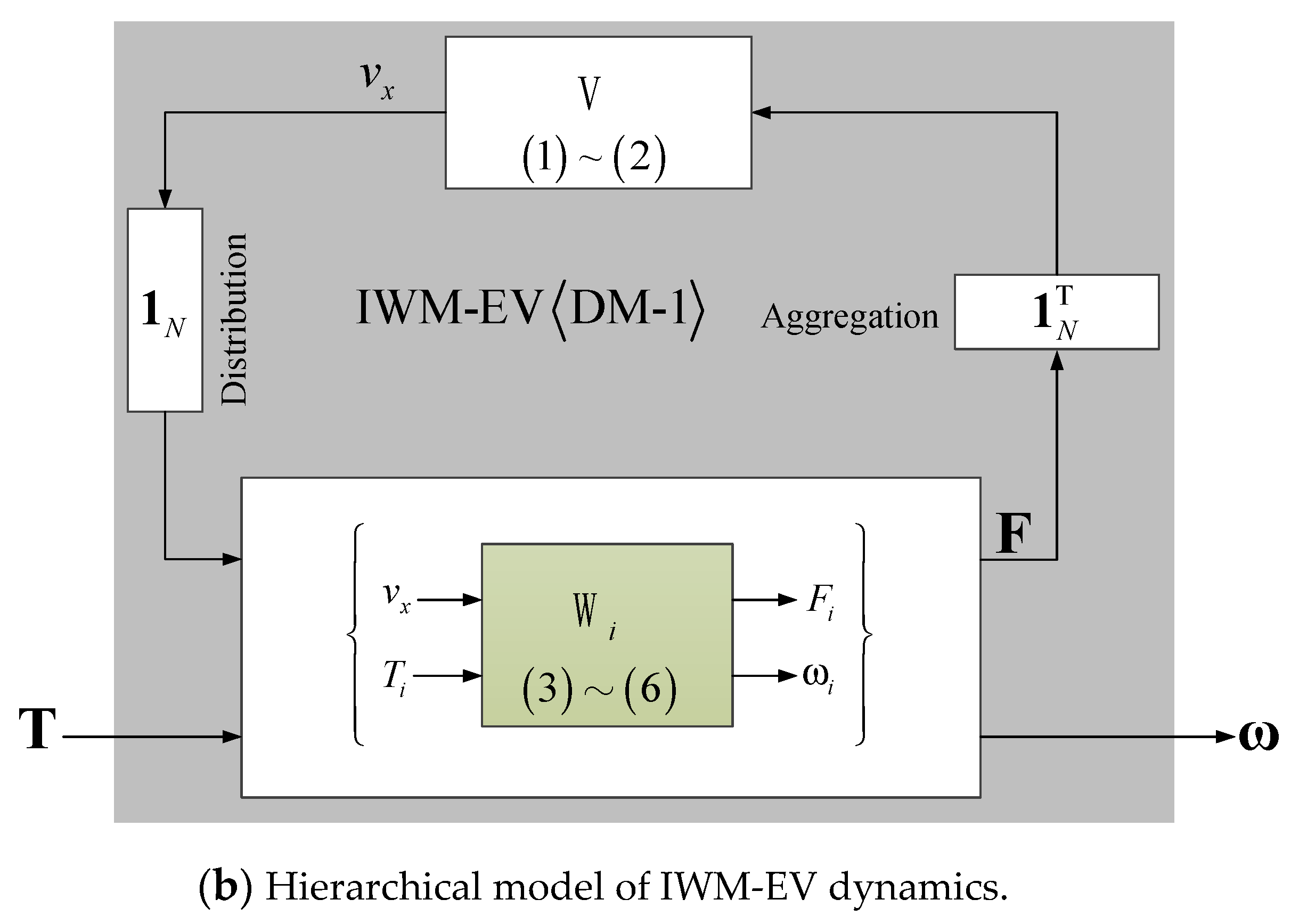
4. DM-1: Nonlinear Model with Hierarchical Structure

This section proposes a way to directly model the IWM-EV system using its nonlinear equations. To design the control system, our strategy is based on the passivity theory which has been widely utilized in various fields of control engineering for three decades. As an example, DM-1 is utilized to design an anti-slip control system. Notice that, it is possible to neglect the disturbance F_ξ in the theoretical discussion.

4.1. Hierarchical Model of IWM-EV

Based on (3)–(6), the model of the local agent W_i is shown as in Figure 6a. It includes two inputs {v_x, T_i} and two outputs {F_i, ω_i}. The vehicle body dynamics V is obtained from (1) and (2). V has the input $1_N^{{\rm T}}F$ which is the aggregation of the local driving force, and the output v_x which is distributed to the local W_i. Combining {W_i} in the lower-layer and V in the upper-layer, the DM-1 is established as in Figure 6b with the hierarchical structure.

4.2. Passivity Theory and Its Application to DM-1

Consider a system given by a state space equation

$$\{\begin{array}{l}\dot{x}=f(x,u)\hfill \\ y=h(x,u)\hfill \end{array},$$

(10)

with the input vector u(t) ∈ ℝ^p, output vector y ∈ ℝ^p, and the state vector x(t) ∈ ℝⁿ.

Definition 1 [41]:

The system (10) is said to be passive from input u to output y if there exists a positive semidefinite function S: ℝⁿ → ℝ₊, called storage function, such that the inequality$\dot{S}\le y^{{\rm T}}u$holds for all x ∈ ℝⁿ and u ∈ ℝ^p. In addition, (10) is input strictly passive (ISP) if $\dot{S}\le y^{{\rm T}}u-{\delta }_u{\Vert u\Vert }^2$ for some δ_u > 0, and output strictly passive (OSP) if $\dot{S}\le y^{{\rm T}}u-{\delta }_y{\Vert y\Vert }^2$ for some δ_y > 0.

Proposition 1:

The IWM-EV system in Figure 6b is passive from the input T to the output ω.

Proof of Proposition 1:

Define the storage function

$$S=\frac{1}{2}m{v}_x^2+{\displaystyle \sum _{i=1}^N\left(\frac{1}{2}{J}_w{\omega }_i^2\right)},$$

(11)

then with respect to Remark 1, it is transparent that the inequality $\dot{S}\le {\mathsf{\omega }}^{{\rm T}}\mathbf{T}$ holds true. The detailed calculation is neglected for the sake of paper length. □

Passivity-based-control (PBC) was introduced three decades ago to the adaptive control problem of rigid robot [45]. It has been widely applied in various fields of control engineering, especially in multi-agent systems [46]. Following the fundamental passivity theorems [41], if the plant is passive, system stability can be guaranteed by connecting the plant with a strictly passive feedback controller. Motivated by the Proposition 1, there exists many ways to design motion control of IWM-EV using PBC [47]. A design example of anti-slip control will be examined in the next subsection.

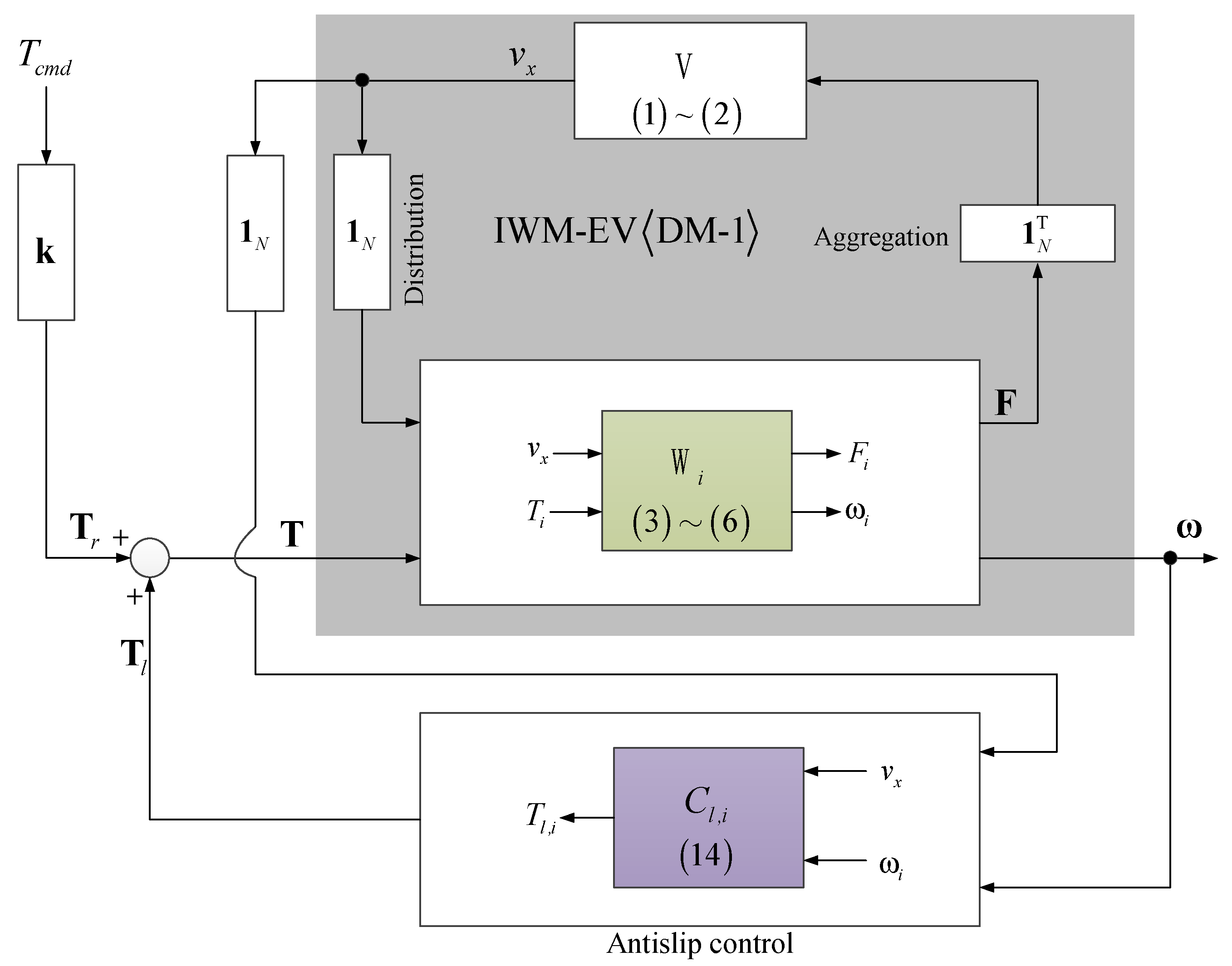
4.3. Example of DM-1: Passivty Based Anti-Slip Control of IWM-EV

This sub-section demonstrates anti-slip control as an application of the DM-1 and passivity theory. The significance and necessity of anti-slip control can be explained from two points of view as follows.

From a safety point of view: As discussed by Hori et al. in [14], not only the driving force but also the side force strongly depends on the slip ratio. The side force becomes smaller as the slip ratio becomes bigger. If the slip ratio increases considerably due to the change of road condition, the side force becomes drastically smaller. This causes serious problems, including drift-out in front-wheel-drive vehicles, spin in rear-wheel-drive vehicles, and drift-out with rotation in four-wheel-drive vehicles. Such situations are extremely dangerous for the drivers.

From an energy point of view: For simplicity in discussion, we consider a single-wheel vehicle model. Following the Proposition 1, its energy storage function is

$$S=\frac{1}{2}m{v}_x^2+\frac{1}{2}{J}_w{\omega }^2,$$

(12)

With respect to the definition of slip ratio expressed in (4), we obtain

$$S=\{\begin{array}{l}\frac{1}{2}\left[m+\frac{J_w}{r^2{\left(1-\lambda \right)}^2}\right]v_x^2\mathrm{if}r\omega >v_x\\ \frac{1}{2}\left[m+\frac{J_w{\left(1+\lambda \right)}^2}{r^2}\right]v_x^2\mathrm{if}r\omega <v_x\end{array},$$

(13)

In the acceleration mode ($r\omega >v_x$), a sharp increasing of λ means a sharp increasing of S. Thus, to attain a given velocity pattern v_x in the acceleration mode, it is required to use more electric energy from the battery. Next, we examine the deceleration mode ($r\omega <v_x$). In this case the side of λ is negative. A drastic decreasing of λ (or increasing of −λ) results in a drastic decreasing of S. Thus, to attain a given velocity pattern v_x in the deceleration mode, only small amount of energy can be regenerated back to the battery. In summary, the driving range of electric vehicles would be considerably reduced if we wasted energy by neglecting anti-slip control.

The proposed control system is shown in Figure 7 where the scalar T_cmd is the driving command given by the driver. The command distributed to each W_i is T_r,i = k_i × T_cmd where the set of distribution ratio satisfies k_i > 0 for all i from 1 to N, and k₁ + k₂ + ... + k_N = 1. Consequently, vectors T_r and k are defined as T_r = [T_r,1 T_r,2 ... T_r,N]^T and k = [k₁ k₂ ... k_N]^T, respectively. Note that vector k can be updated in real-time to attain the additional control objective, such as yaw moment control or minimization of energy consumption. Let K_a and K_ω be the control gains. Considering the acceleration mode, a possible option of the local anti-slip control law C_l,i is given by

$$T_{l,i}=-K_a\left(r{\omega }_i-v_x\right)sign\left({\omega }_i\right)sign\left(r{\omega }_i-v_x\right)-K_{\omega }{\omega }_i.$$

(14)

The stability of the control system is guaranteed by the following theoretical result.

Proposition 2:

Considering the acceleration mode, the anti-slip control system inFigure 7 with the local controller C_l,i given by (14) is OSP from T_r to ω if the control gains are selected such that K_a > 0 and K_ω > 0.

Proof of Proposition 2:

With respect to the storage function (11), the control law (14), and the dynamics of W_i described by (3)–(6), we have

$$\begin{array}{l}{\mathsf{\omega }}^{{\rm T}}{T}_r-\dot{S}={\displaystyle \sum _{i=1}^N\left(\max \left\{r{\omega }_i,v_x,\epsilon \right\}{\lambda }_i{f}_i({\lambda }_i)\right)}+\left(\rho \left|v_x\right|\right)v_x^2\\ +{\displaystyle \sum _{i=1}^N{K}_a\left(\left(r{\omega }_i-v_x\right)sign\left(r{\omega }_i-v_x\right)\right)\left({\omega }_{i}sign\left({\omega }_i\right)\right)}+{\displaystyle \sum _{i=1}^N{K}_{\omega }{\omega }_i^2}\end{array}$$

(15)

□

There exist four terms on the right-hand side of (15). It is clear from Remark 1 that the first term is non-negative. Similarly, the second term is non-negative. With the positive control gains, we can see that ${\mathsf{\omega }}^{{\rm T}}{T}_r-\dot{S}\ge {\displaystyle \sum _{i=1}^N{K}_{\omega }{\omega }_i^2}=K_{\omega }\left({\mathsf{\omega }}^{{\rm T}}\mathsf{\omega }\right)$ holds true. In other words, $\dot{S}\le {\mathsf{\omega }}^{{\rm T}}{T}_r-K_{\omega }\left({\mathsf{\omega }}^{{\rm T}}\mathsf{\omega }\right)$. Following the Definition 1, the system in Figure 7 is shown to be OSP. This completes the proof.

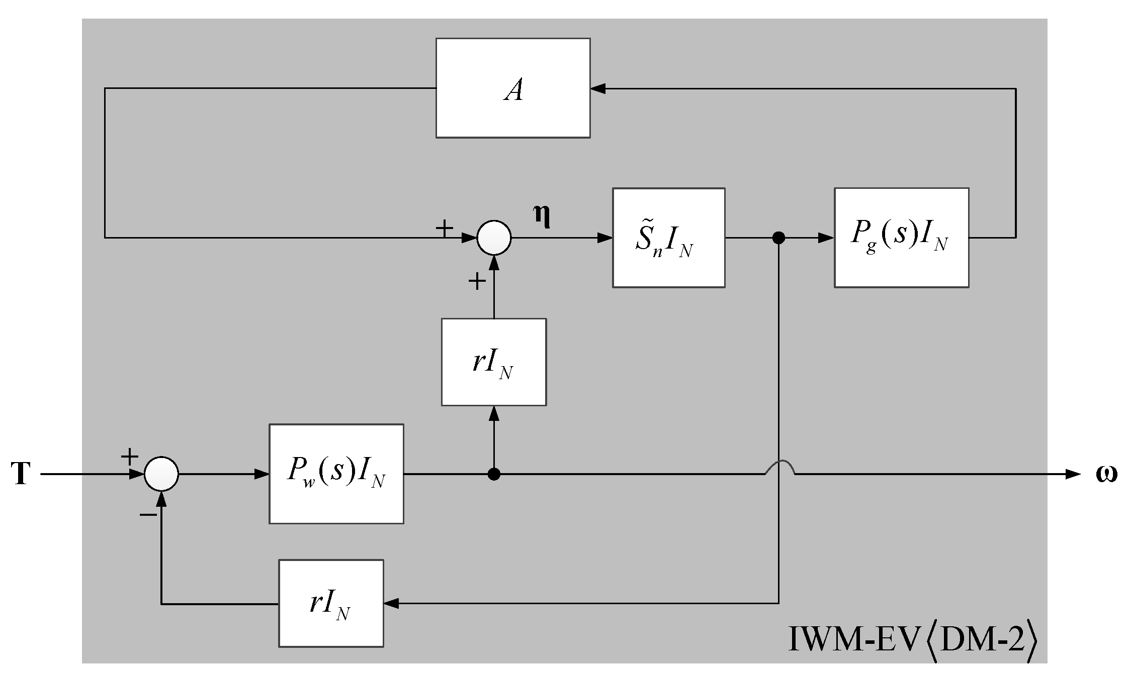
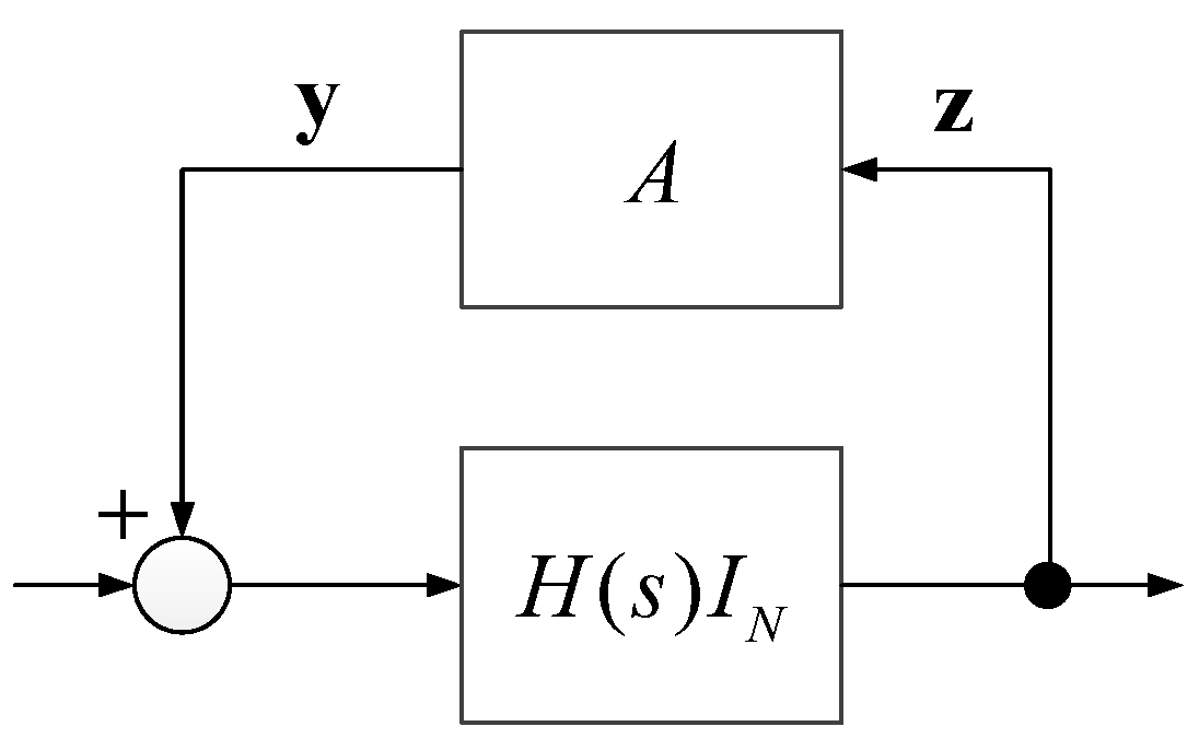
5. DM-2: Linearized Model with Rank-1 Interconnection Matrix

The previous section focuses on the design problem using DM-1. Thanks to the passivity theory, we can rigorously prove the stability of the control system even if it is nonlinear and quite complex. However, passivity theory limits the class of controllers that we can select. Therefore, it is also essential to consider the problem of stability analysis. In other words, given a motion control system, how should we evaluate its stability? This section introduces a design model which can reduce the complexity level of the analysis problem. As an example, it is applied to a wheel velocity control system of IWM-EV. Note that, the air resistance and the other disturbances are neglected in the discussion in this section. For the sake of paper length, we only examine the vehicle motion in the acceleration mode, such that max{rω_i, v_x, ε} = rω_i. We focus our stability analysis to the operating point O = {ω_o,1, ω_o,2, …, ω_o,N, v_xo} with the following assumption.

Assumption 1:

(i) The vehicle operates on the uniform road condition and the friction coefficients of all wheels are the same. (ii) The slip ratio is small, and the driving force is linearized asF_i≈S_nλ_iwhereS_nis the nominal driving stiffness. At O, the values of max{rω_o,i, v_xo, ε} are almost the same. In other words, we might approximate

$${\kappa }_n\approx \frac{1}{\max \left\{r{\omega }_{\mathrm{o},i},v_{x\mathrm{o}},\epsilon \right\}}\forall i\in \left[1,N\right].$$

(16)

5.1. Linearized Model of IWM-EV

Under the Assumption 1, the driving force can be expressed as

$$F_i={\tilde{S}}_n{\eta }_i,$$

(17)

where ${\tilde{S}}_n\approx {\kappa }_n{S}_n$, and ${\eta }_i=r{\omega }_i-v_x$. Based on (17), the linearized model of IWM-EV (DM-2) is established as in Figure 8 where η = [η₁ … η_N]^T and

$$A=-1_N{1}_N^{{\rm T}},$$

(18)

$$P_g(s)=\frac{1}{ms},P_w(s)=\frac{1}{J_{w}s}.$$

(19)

Remark 2:

The interconnection matrixAis a matrix of rank-1 withN-1 zero eigenvalues, and only one non-zero eigenvalue which equals to -N.

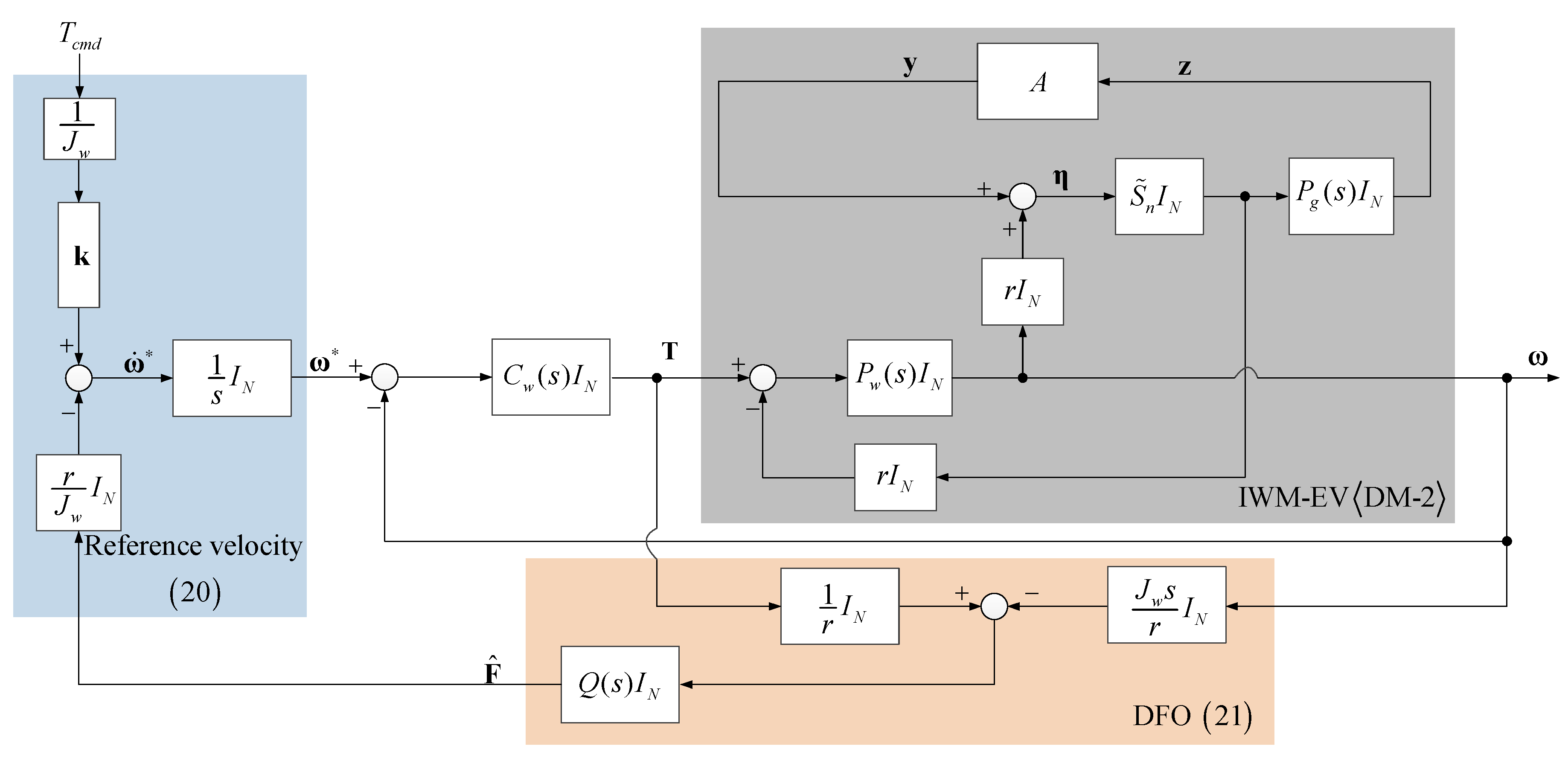
5.2. Example of DM-2: Wheel Velocity Control System and Its Stability Condition

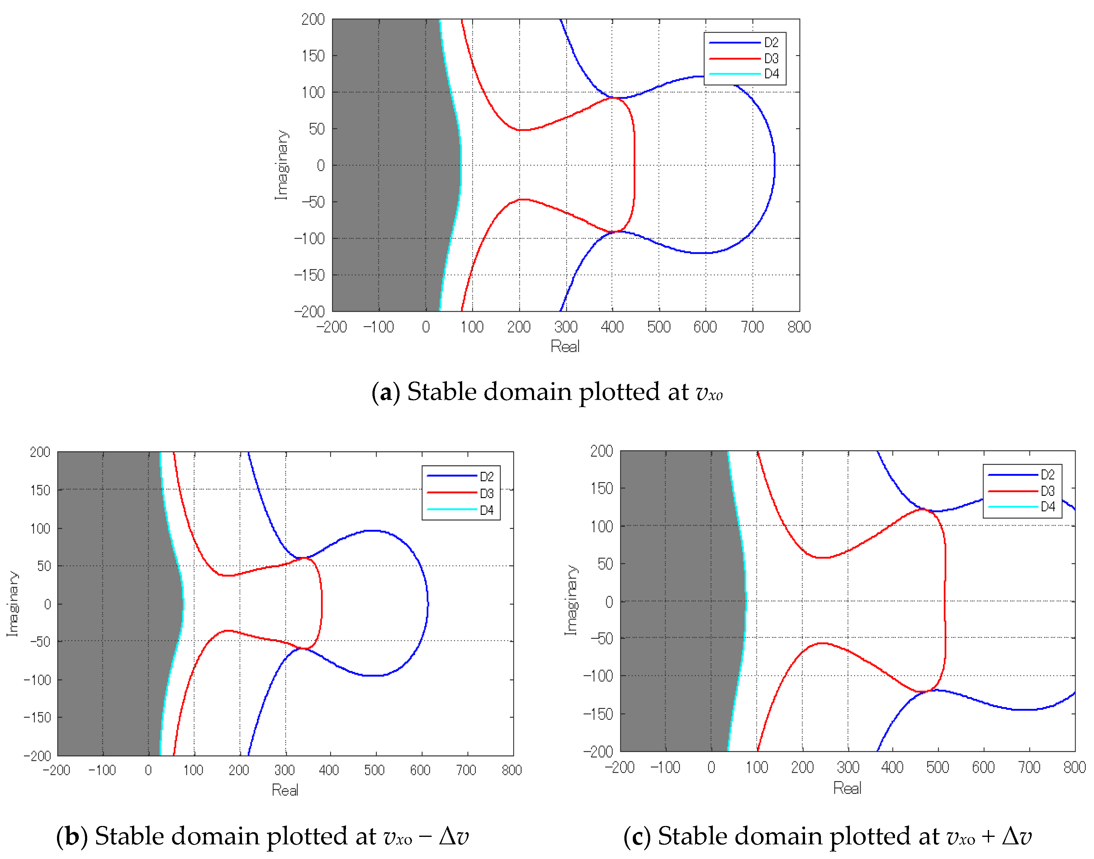
This section considers a wheel velocity control system for distributing the driving command T_cmd with a set of distribution ratios {k_i}. From (3), the reference of wheel acceleration is calculated as [48]

$${\dot{\omega }}_i^{\ast }=\frac{1}{J_w}{k}_i{T}_{cmd}-\frac{r}{J_w}{\widehat{F}}_i,$$

(20)

where ${\widehat{F}}_i$ is the obtained by the driving force observer (DFO) as follows

$${\widehat{F}}_i=Q(s)\cdot \left(\frac{1}{r}{T}_i-\frac{J_w}{r}\cdot s\cdot {\omega }_i\right),$$

(21)

where the low-pass-filter is expressed as Q(s) = 1/(τ_fs + 1) with the small time constant τ_f. From (19)–(21) and the DM-2, block diagram of the wheel velocity control system is shown in Figure 9 where C_w(s) is the wheel velocity controller. Notice that we neglect to discuss the algorithms to optimize in this section. Such algorithms can be founded in several other works on range extension control of IWM-EV [48,49,50]. The main goal of this section is to provide a suitable model for stability analysis. About the operating point O, the stability of the system in Figure 9 can be discussed from the system in Figure 10 where the transfer function from y to z is diagonalized by

$$H(s)=\frac{{\tilde{S}}_n\left(1+{\tilde{C}}_w(s)P_w(s)\right)P_g(s)}{1+{\tilde{C}}_w(s)P_w(s)+{\tilde{S}}_n{r}^2{P}_w(s)},{\tilde{C}}_w(s)=\frac{C_w(s)\left(1-Q(s)\right)}{1+C_w(s)P_w(s)Q(s)}.$$

(22)

The system in Figure 10 is a multi-agent-system of N agent H(s), interconnecting via the matrix A. The system is stable at O if and only if

$${\nu }_{i}H(s)-1\ne 0\forall \hspace{1em}s\in {ℂ}_{+},$$

(23)

for all eigenvalues ${\nu }_i$ of matrix A. We notice that the zero eigenvalues certainly satisfy (23). Following the generalized frequency variable theory (GFV) [35] with respect to Remark 2, (23) can be checked by the following condition.

Stability condition 1:

The wheel velocity control system is stable at the operating point O if the point (-N, 0) is located in the stable domain${\mathsf{\Omega }}_{+}^c$defined as${\mathsf{\Omega }}_{+}:=\varphi \left(C_{+}\right),{\mathsf{\Omega }}_{+}^c:=C\backslash {\mathsf{\Omega }}_{+}$where the GFV is$\varphi (s)=H^{-1}(s)$.

5.3. Stability Test

To demonstrate the Stability condition 1, this section considers the PI controller

$$C_w(s)=\frac{K_{P}s+K_I}{s}.$$

(24)

Substitute (24) to (22), the transfer function of the GFV is derived as

$$\varphi (s)=\frac{1}{H(s)}=\frac{s^4+a_3{s}^3+a_2{s}^2+a_{1}s+a_0}{b_3{s}^3+b_2{s}^2+b_{1}s+b_0},$$

(25)

where the set of {a_i, b_i} is expressed in the Appendix B. Define the polynomial

$$pl=s^4+a_3{s}^3+a_2{s}^2+a_{1}s+a_0-\left(x+jy\right)\left(b_3{s}^3+b_2{s}^2+b_{1}s+b_0\right)\equiv s^4+{\displaystyle \sum _{i=1}^4(p_i+j{q}_i)s^{4-i}}.$$

(26)

Following the Theorem 1 in [35], a set of {D_k > 0} that defining the stable domain is obtained as

$$\{\begin{array}{l}{D}_1=\det \left|p_1\right|\hfill \\ D_k=\det \left[\begin{array}{cc}F(p_k)& -F(q_k)R\\ UF(q_k)& F(p_{k-1})\end{array}\right](k=2,\dots ,4)\hfill \end{array},$$

(27)

where

$$p_k={\left[\begin{array}{lllll}1\hfill & p_1\hfill & p_2\hfill & \dots \hfill & p_{2k-1}\hfill \end{array}\right]}^T,q_k={\left[\begin{array}{llllll}0\hfill & 0\hfill & q_1\hfill & q_2\hfill & \dots \hfill & q_{2k-2}\hfill \end{array}\right]}^T,$$

$$R=\left[\begin{array}{c}0\\ I\end{array}\right]\in {ℝ}^{k\times (k-1)},U=\left[\begin{array}{cc}I& 0\end{array}\right]\in {ℝ}^{(k-1)\times k},F(x)=\left[\begin{array}{lllll}{x}_2\hfill & x_4\hfill & x_6\hfill & \dots \hfill & x_{2k}\hfill \\ x_1\hfill & x_3\hfill & x_5\hfill & \ddots \hfill & ⋮\hfill \\ 0\hfill & x_2\hfill & x_4\hfill & \ddots \hfill & x_{k+3}\hfill \\ ⋮\hfill & \ddots \hfill & \ddots \hfill & \ddots \hfill & x_{k+2}\hfill \\ 0\hfill & \dots \hfill & 0\hfill & x_{k-1}\hfill & x_{k+1}\hfill \end{array}\right].$$

Notice: p_i = q_i = 0 if i > 4.

Based on the GFV theory [35], the Stability condition 1 can be tested as follows.

Stability test 1:

We consider an operating point O = {ω_o,1, ω_o,2, …, ω_o,N, v_xo}. We establish the linearized model DM-2 under the Assumption 1. We calculate the GFV using (25), and then establish the set of {D_k} using (26) and (27). The wheel velocity control system in Figure 9 is stable at O if

$$D_k(x=-N,y=0)>0\forall k\in \left\{1,2,3,4\right\}.$$

(28)

The complexity level of the Stability test 1 is independent of the number of IWM actuators. At each operating point, the test is performed by a limited set of inequalities (28).

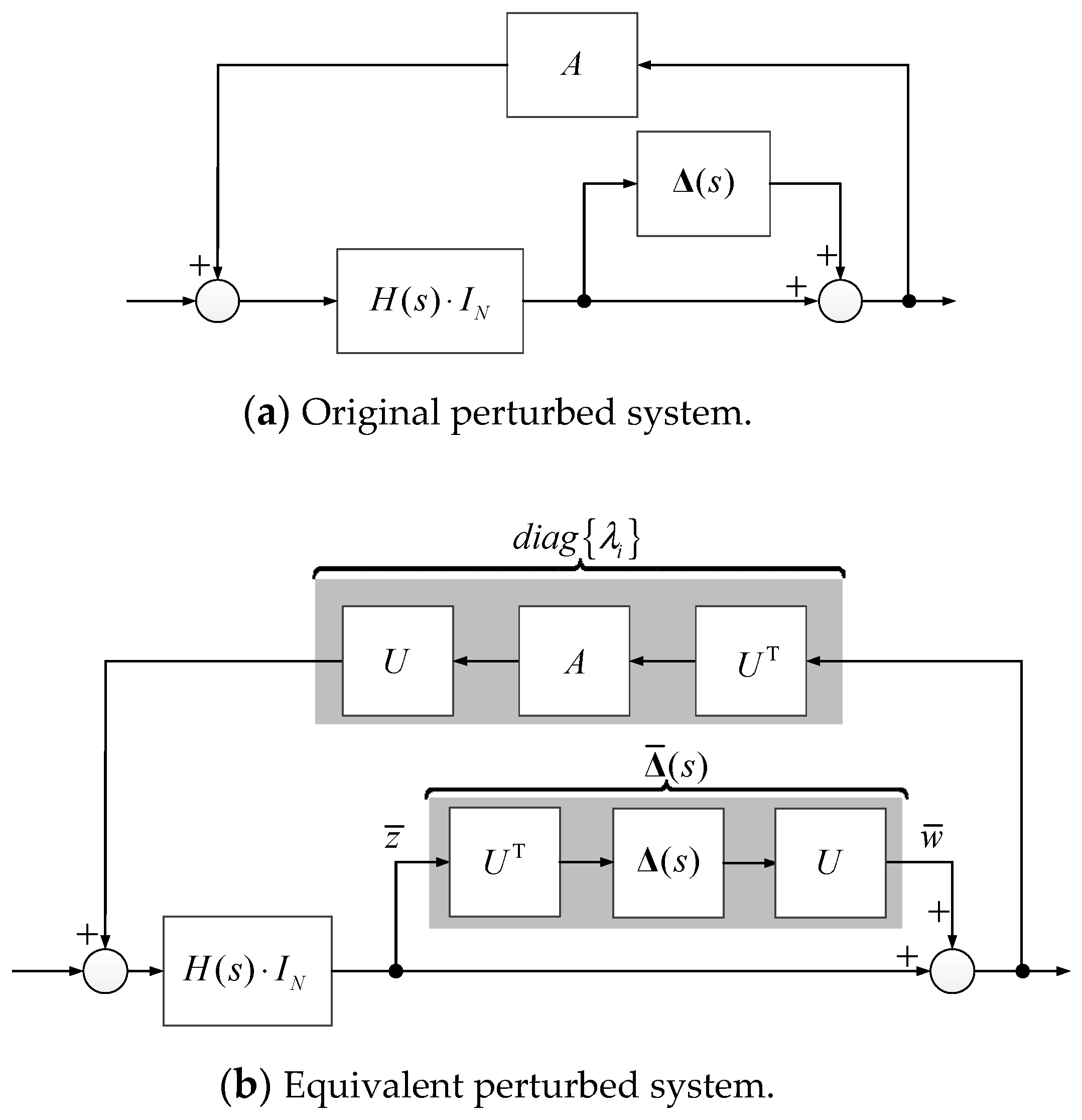
5.4. Discussion: Possibility of Robust Stability Test

By using Assumption 1, the LMC system of electric vehicle is finally modelled as a homogeneous multi-agent system as in Figure 10. However, in actual operation, the friction coefficients of all wheel might be not the same. In addition, the friction coefficients might vary due to the change of road condition. Considering this scenario, we can express the LMC system as a multi-agent system with perturbation as in Figure 11a. The perturbation matrix is Δ(s) = diag{Δ_i(s)}. We can assume that each local perturbation satisfies ${\Vert {\Delta }_i(s)\Vert }_{\infty }\le \xi$ where the volume $\xi$ of perturbation represents the heterogeneous level between the agents and the uncertainties due to the change of road condition. With respect to the structure of matrix A given by (18), there exists the unitary matrix U that diagonalizes matrix A. Thus, we can transform the system in Figure 11a to the equivalent system in Figure 11b where {${\lambda }_i$} is the set of eigenvalues of matrix A. The transfer function from $\overline{w}$ to $\overline{z}$ is diagonalized by N transfer functions

$${\overline{H}}_i(s)=\frac{{\lambda }_{i}H(s)}{1-{\lambda }_{i}H(s)}.$$

(29)

As ${\Vert {\Delta }_i(s)\Vert }_{\infty }\le \xi$, it follows that $\left|\right|\Delta (s)|{|}_{\infty }\le \xi$, and therefore $\left|\right|\overline{\Delta }(s)|{|}_{\infty }\le \xi$ since U is a unitary matrix. Applying the small gain theorem, the perturbed system is robust stable if

$${\Vert \frac{{\lambda }_{i}H(s)}{1-{\lambda }_{i}H(s)}\Vert }_{\infty }\le \frac{1}{\xi }\forall {\lambda }_i\in \sigma \left(A\right).$$

(30)

The zero eigenvalues certainly satisfy (30). With respect to Remark 2, the robust stability condition is reduced to

$${\Vert \frac{N{H}_n(s)}{1+N{H}_n(s)}\Vert }_{\infty }\le \frac{1}{\xi }.$$

(31)

In summary, the DM-2 is still applicable to deal with the uncertainties. In this situation, we have to design for each wheel a local controller such that a triad of conditions are satisfied: (i) the stability condition of the nominal system given by (28); (ii) the model matching condition given by the norm inequality ${\Vert {\Delta }_i(s)\Vert }_{\infty }\le \xi$; and (iii) the robust stability condition given by (31).

Another way to deal with robust stability is to utilize “sector bounded nonlinearity” of the tire-force characteristics (Figure 12). We can directly apply the Circle and Popov criteria which was presented in Khalil’s famous book on nonlinear control [41]. Fortunately, the special structure of matrix A could be utilized to reduce the complexity of “Circle and Popov criteria”. We let this discussion for future study, as the goal of this paper is only to discuss several ways to model the vehicle dynamics such that longitudinal motion control can be designed properly.

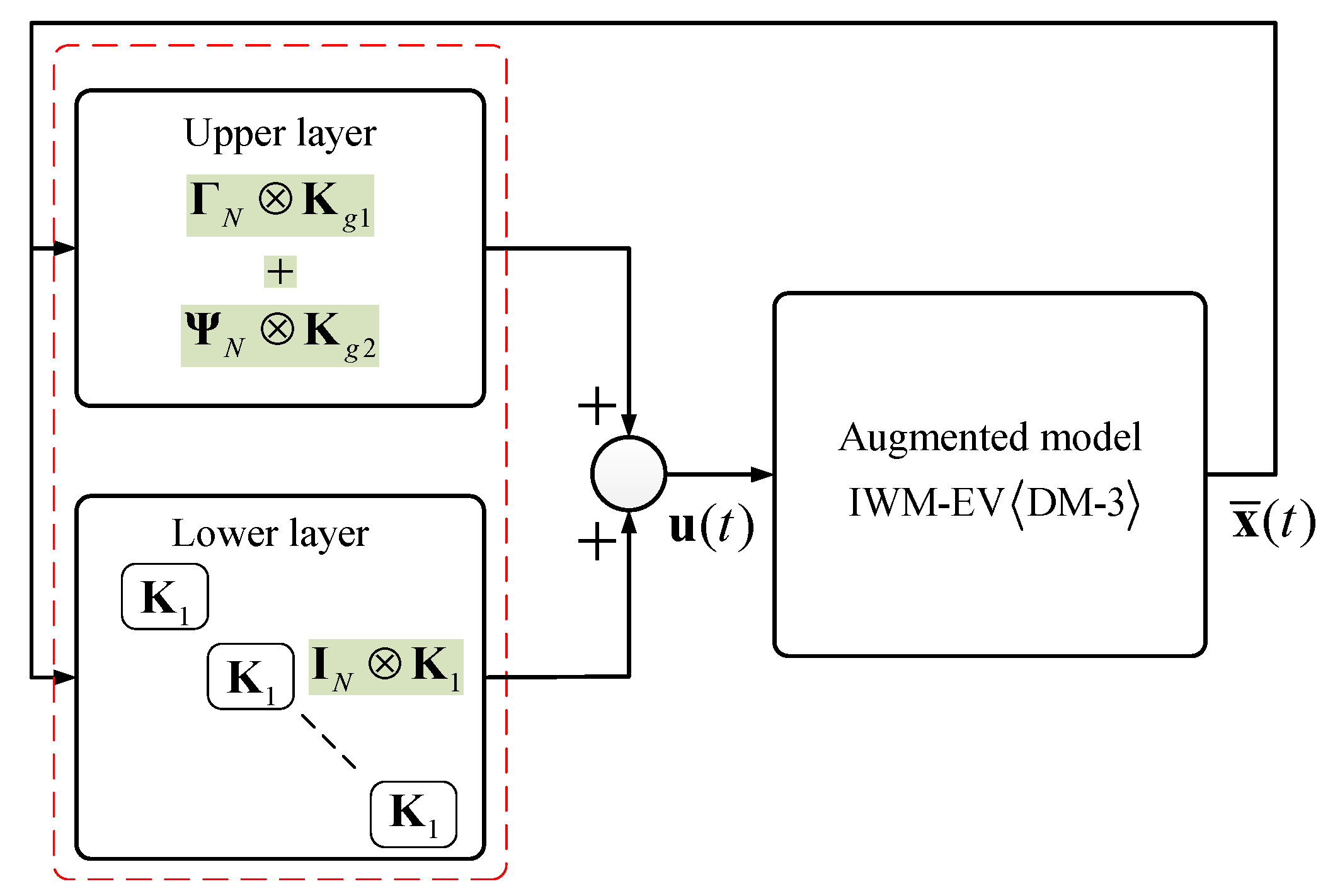
6. DM-3: Time-Varying State-Space Model

In Section 4, the DM-1 is established based on the "physical equations" of the IWM-EV. Section 5 proposes the DM-2 expressed by "transfer functions and interconnection matrix". This section shows that the dynamics of IWM-EV can also be captured by a "state-space model". We examine the vehicle motion in the deceleration mode, such that max{rω_i, v_x, ε} = v_x. Notice that it is possible to neglect the unknown disturbances of F_air and F_ξ in the expression of this model.

6.1. State-Space Model of IWM-EV in the Deceleration Mode

Calculating the derivative of the slip ratio (4) with respect to (1) and (3), we have

$${\dot{\lambda }}_i=-\frac{r^2}{J_w{v}_x}{F}_i-\frac{{\dot{v}}_x}{v_x}{\lambda }_i+\frac{r}{J_w{v}_x}{T}_i-\frac{1}{m{v}_x}{\displaystyle \sum _{j=1}^N{F}_j}.$$

(32)

For the sake of estimation and control design, it is possible to use the first order dynamics model [51] of the driving force represented by

$${\tau }_i{\dot{F}}_i+F_i=S_i{\lambda }_i,$$

(33)

where ${\tau }_i$ is the relaxation time constant and S_i is the driving stiffness which is a parameter for capturing the linear region of the Pacejka model. Here, S_i can be identified from IWM’s torque and on-board sensor [52]. Selecting the slip ratio and driving force as state variables, and considering wheel velocities as time-varying parameter, from (30) and (31), the dynamical equation of the ith agent is expressed as follows

$${\dot{x}}_i(t)=A_{l,i}(t)x_i(t)+B_{l,i}{u}_i(t)+{\displaystyle \sum _{j=1}^N{A}_{g,ij}(t)x_j(t)},$$

(34)

where

$$x_i(t)={\left[\begin{array}{cc}{F}_i(t)& {\lambda }_i(t)\end{array}\right]}^T,u_i(t)=T_i(t),$$

(35)

$$A_{l,i}(t)=\left[\begin{array}{cc}\frac{-1}{{\tau }_i}& \frac{S_i}{{\tau }_i}\\ \frac{-r^2}{J_w{v}_x}& \frac{-{\dot{v}}_x}{v_x}\end{array}\right],B_{l,i}(t)=\left[\begin{array}{c}0\\ \frac{r}{J_w{v}_x}\end{array}\right],A_{g,ij}(t)=\left[\begin{array}{cc}0& 0\\ -\frac{1}{m{v}_x}& 0\end{array}\right].$$

(36)

Define $x(t)={\left[\begin{array}{ccc}{x}_1^T(t)& \dots & x_N^T(t)\end{array}\right]}^T$ and $u(t)={\left[\begin{array}{ccc}{u}_1^T(t)& \dots & u_N^T(t)\end{array}\right]}^T$, the DM-3 is expressed as

$$\dot{x}(t)=\left(A_L(t)+A_G(t)\right)x(t)+B_L(t)u(t),$$

(37)

where $A_L(t)=diag\left\{A_{l,i}(t)\right\},B_L(t)=diag\left\{B_{l,i}(t)\right\},A_G(t)=\left\{A_{g,ij}(t)\right\}$. The full block matrix A_G(t) represents the physical interaction between the local agents.

The acceleration-mode-version of DM-3 when max{rω_i, v_x, ε} = rω_i can be found in our recent study [17]. DM-3 can be used for controlling either driving force or slip ratio. To this end, we proposed in [17] a hierarchically decentralized LQR algorithm which was verified by real-time experiments using an EV driven by two IWMs.

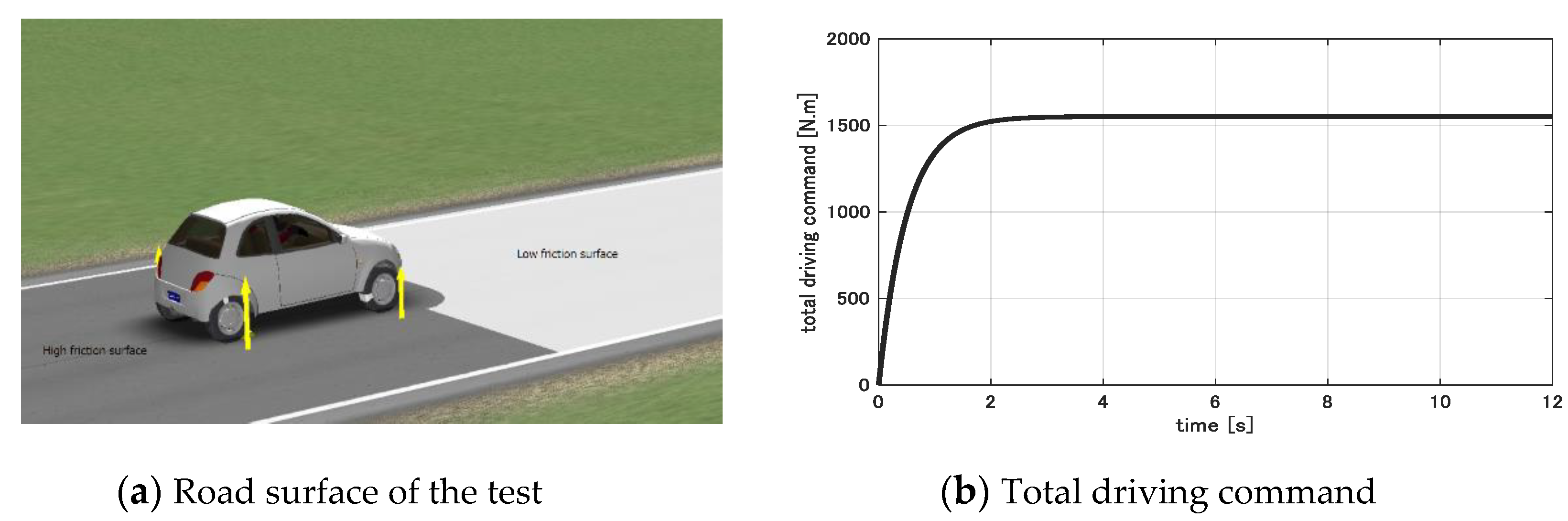
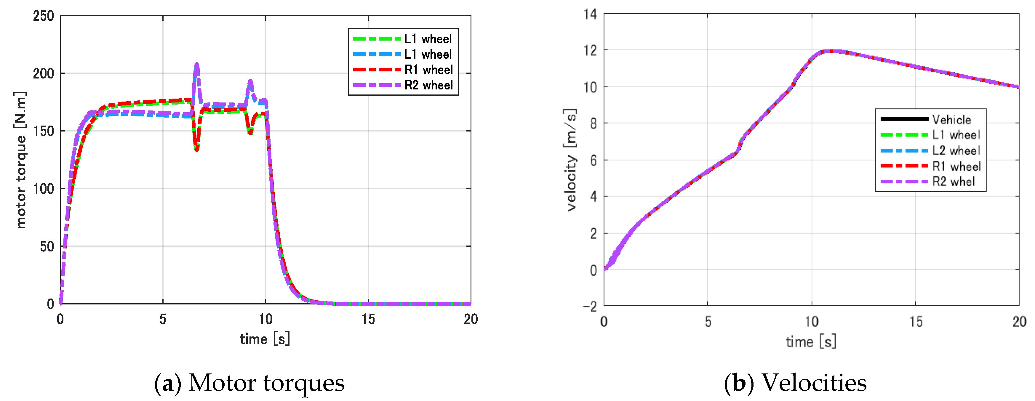
6.2. Example of DM-3: Slip Ratio Control in the Deceleration Mode

To demonstrate the practical application of DM-3, we investigate the slip ratio control in the deceleration mode. The following assumptions are considered for the sake of simplicity in presenting our main idea.

Assumption 2:

All the state variables and time-varying parameters of the system (34) or their appropriate estimates are available.

Assumption 3:

The parameters {${\tau }_i$, S_i} are not much different from wheel to wheel, and we can represent them by the nominal parameters {${\tau }_n$, S_n}.

Assumption 2 is reasonable since the driving force can be estimated accurately using DFO presented in the previous section. From DFO and the estimated/calculated slip ratio, the driving stiffness can be identified off-line or on-line [52]. On the other hand, the vehicle velocity and wheel slip ratio can be estimated using on-board sensor, such as GPS receiver, accelerometer, and wheel encoders. Several methods for estimating slip ratio can be found in [17,53]. We neglect to focus on state estimation and parameter identification, since it is not the main goal of this paper.

The parameters {${\tau }_i$, S_i} depend on the road condition at each wheel and load transfer. This means the parameters {${\tau }_i$, S_i} are not always the same in real-time operation. The Assumption 3 is reasonable if the wheels are symmetrically distributed in the vehicle body, and the local road conditions of the wheels are quite uniform. Since we implement the feedback control using DM-3, the parameter difference among the local agents can be compensated.

For controlling the slip ratios such that they follow the reference value ${\lambda }_i^{*}$, the tracking errors are introduced as the augmented states. In the following, time stamping “t” is eliminated for simplifying the expression. The augmented dynamical model of the ith agent is given as

$${\dot{\overline{x}}}_i={\overline{A}}_1{\overline{x}}_i+{\overline{B}}_1{u}_i+{\displaystyle \sum _{j=1}^N{\overline{A}}_2{\overline{x}}_j}+{\overline{G}}_{\lambda }{\lambda }_i^{*},$$

(38)

where ${\overline{x}}_i={\left[\begin{array}{ccc}{F}_i& {\lambda }_i& e_i\end{array}\right]}^T,e_i={\displaystyle \int \left({\lambda }_i-{\lambda }_i^{*}\right)dt}$ and

$${\overline{A}}_1=\left[\begin{array}{ccc}-\frac{1}{{\tau }_n}& \frac{S_n}{{\tau }_n}& 0\\ -\frac{r^2}{J_w{v}_x}& -\frac{-{\dot{v}}_x}{v_x}& 0\\ 0& 1& 0\end{array}\right],{\overline{B}}_1=\left[\begin{array}{c}0\\ \frac{r}{J_w{v}_x}\\ 0\end{array}\right],{\overline{A}}_2=\left[\begin{array}{ccc}0& 0& 0\\ -\frac{1}{m{v}_x}& 0& 0\\ 0& 0& 0\end{array}\right],{\overline{G}}_{\lambda }=\left[\begin{array}{c}0\\ 0\\ -1\end{array}\right].$$

State-space modelling of the total system is expressed as follows using Kronecker product $\otimes$:

$$\dot{\overline{x}}=\overline{A}\overline{x}+\overline{B}u+\overline{G}{\lambda }^{\ast },$$

(39)

where $\overline{x}={\left[\begin{array}{ccc}{\overline{x}}_1^T& \dots & {\overline{x}}_N^T\end{array}\right]}^T,{\lambda }^{\ast }={\left[\begin{array}{ccc}{\lambda }_1^{\ast }& \dots & {\lambda }_N^{\ast }\end{array}\right]}^T$ and

$$\overline{A}=I_N\otimes {\overline{A}}_1+{\Gamma }_N\otimes {\overline{A}}_2,{\Gamma }_N=1_N{1}_N^T,\overline{B}=I_N\otimes {\overline{B}}_1,\overline{G}=I_N\otimes {\overline{G}}_{\lambda }.$$

The LQR controller of the augmented system (39) can be obtained by minimizing the quadratic cost function

$$\Im ={\displaystyle \underset{t_o}{\overset{t_f}{\int }}{\overline{x}}^{T}Q\overline{x}dt}+{\displaystyle \underset{t_o}{\overset{t_f}{\int }}{u}^{T}Rudt}+x_f^{T}H{x}_f,$$

(40)

where t₀ is the initial time, t_f is the finished time. Q and S are symmetric positive semidefinite matrices, and R is strictly symmetric positive definite matrix. Q, H, and R are used to penalize the transient state deviation, the final state, and the control effort, respectively. By solving the Riccati equation

$$\dot{P}+P\overline{A}+{\overline{A}}^{T}P-P\overline{B}{R}^{-1}{\overline{B}}^{T}P+Q=0,$$

(41)

that satisfies the boundary condition

$$P_f\triangleq P\left(t_f\right)=H,$$

(42)

the control gain is obtained as

$$K=-R^{-1}{\overline{B}}^{T}P,$$

(43)

Equation (41) with condition (42) can be solved using the Hamiltonian established from the system model [54]. To reduce the computational effort, especially when N is a big number, we recently proposed in [17] that the feedback gain can be calculated as

$$K=I_N\otimes K_1+{\Gamma }_N\otimes K_{g1}+{\Psi }_N\otimes K_{g2},$$

(44)

by appropriate choices of the weighting matrices. As can be seen in Figure 13, the proposed LQR controller has the hierarchical structure. In the lower layer, the local feedback gain K₁ is used to improve the local control performance of slip ratio. The upper-layer has two term, K_g1 and K_g2. K_g1 is to deal with the physical interconnection represented by ${\Gamma }_N$. On the other hand, K_g2 is introduced to improve some other global performances, such as the consensus of slip ratios. Since K₁ is obtained by solving the Riccati equation of a local system, the computation cost is independent of the number of IWM actuators. See Appendix C for the details of the hierarchical LQR algorithm.

Notice 1:

Similar to Assumption 1, Assumption 3 is just to limit our discussion to homogenous multi-agent systems. Motivated by a recent work of Nguyen and Hara [33], we will develop the H-LQR version for heterogeneous multi-agent systems with physical interaction in our future study.

7. Evaluation of the Proposed Design Models by Carsim/Matlab Co-Simulator

Using the Carsim/Matlab co-simulator introduced in Section 3, this section is to demonstrate the effectiveness of the proposed design models.

7.1. Evaluation of Passivity Based Anti-Slip Control Using DM-1

To evaluate the proposed anti-slip control strategy, a test is conducted as follows. As shown in Figure 14a, the EV accelerates from the initial position on the high friction surface (μ = 0.8). It enters the low friction surface (μ = 0.2) at about 5.7 s. The total driving command T_cmd is expressed in Figure 14b. The distribution vector k is updated to minimize the total workload of all wheels [55].

Case 1 (Without anti-slip control: Figure 15): The motor torque of each wheel is only distributed from the total driving command, i.e., T_i = k_iT_cmd where k_i is the distribution ratio of the ith wheel. Consequently, the slip occurs. Especially, the rear-wheel velocities increase considerably as the vehicle enters the low friction surface.

Case 2 (With passivity-based anti-slip control: Figure 16): The anti-slip control law is implemented based on passivity and the DM-1. By trial-and-error, we select the control gains K_a = 100 and K_ω = 0.0001. Notice that a small positive value of K_ω is enough to assure the strict passivity of the control system. We should not select a big value of K_ω which certainly degrades the acceleration performance of the vehicle. In contrast to Case 1, the motor torques are generated properly on different road surfaces. Thus, the wheel velocities are always closed to the vehicle velocity.

The above test cases clarify the merit of the proposed anti-slip strategy using DM-1. Although the physical system of the EV is quite complex and nonlinear, it can be modelled hierarchically with the aggregation and distribution. Based on this model, we can analyze the passivity of the EV dynamics, and design the anti-slip control law that rigorously guarantees the stability of the overall system. Thanks to passivity theory, we design the system with less mathematical and computational effort. Using the DM-1, the energy storage function of the EV is shown to be $S=\frac{1}{2}m{v}_x^2+{\displaystyle \sum _{i=1}^N\left(\frac{1}{2}{J}_w{\omega }_i^2\right)}$. Given a desired velocity pattern of v_x, the energy consumption of the EV can be reduced if the longitudinal velocities of the wheels {rω_i} are closed to v_x. Therefore, the proposed anti-slip control is not only for improving the safety, but also extending the use of the energy source for the EVs.

7.2. Evaluation of GFV Based Stability Analysis Using DM-2

To demonstrate the GFV based stability analysis using DM-2, we conducted wheel velocity control using the system in Figure 9. The EV operates on the high friction surface with μ = 0.85, as shown in Figure 17a. The total driving command T_cmd is expressed in Figure 17b. Similar to the previous sub-section, the distribution vector k is updated to minimize the total workload of all wheels. The driving force observer is designed with the time constant τ_f = 0.033 [s]. This paper examines the operating points with v_xo = 10 (m/s). Considering the high friction surface, it is reasonable to assume that a small slip ratio of 0.05 is maintained constantly when the vehicle velocity changes between v_xo − Δv and v_xo + Δv where Δv = 2 (m/s). We select the wheel velocity controller with {K_p =52.8; K_i = 528.0}. It is transparent that this controller stabilizes the local transfer function H(s) about the operating points. Applying the Stability test 1, the stability regions at the operating points of v_xo, v_xo − Δv and v_xo + Δv are plotted as the shaded regions in Figure 18a–c, respectively. It is transparent that the points (−4, 0) and (0,0) are always placed in such shaded regions. This means the wheel velocity control system in Figure 9 is stable at the aforementioned operating points.

The above example of stability test unveils a merit of GFV approach using DM-2. Thanks to the rank-1 physical interaction expressed by DM-2 and the GFV theory, the complexity of the stability test is independent of the number of IWM actuators. We can repeat the above test to assure the stability of the control system at different operating points with the vehicle velocity from zero to v_xo. This statement is confirmed again by the simulation results summarized in Figure 19. In this simulation, the vehicle is accelerated until 10 s. From 10 s, the total driving command becomes zero, and the vehicle is gradually decelerated due to friction.

In Appendix D, we present several results of the real-time experiments of the wheel velocity control system in Figure 9.

7.3. Evaluation of LQR-Based Slip-Ratio Control Using DM-3

Using the DM-3, we proposed the LQR algorithm for controlling slip-ratio of IWM-EV [17]. This algorithm is verified in the acceleration mode. We also compared the performance of the LQR algorithm with the others, such as sliding mode algorithm and model-following algorithm in [17]. This comparison presented the merits of the proposed LQR: (i) As a hierarchically decentralized algorithm, its computational cost is considerably reduced in comparison with the conventional centralized LQR. (ii) Unlike the completely decentralized control algorithms, the physical interaction between the local wheels are properly treated. This gives the degree of freedom to improve the consensus of local wheels’ slip ratios. In addition, this can reduce the vibration of slip ratios introduced by the non-flat surfaces. (iii) The optimal control gains can be updated at every control period by the measurements of vehicle motion (vehicle velocity, wheel velocities, driving forces).

For the sake of paper space, we neglect to repeat the comparison between the control approaches in this study. Instead, we only demonstrate the performance of the proposed algorithm in deceleration mode (Figure 20a). A total driving command is given as in Figure 20b. This command is distributed to the local wheels to minimize the total workload. The vehicle runs on high friction surface (μ = 0.8) from the beginning until 12 s. From 12 s, the vehicle starts to decelerate on the low friction surface (μ = 0.2). The proposed LQR algorithm is applied to maintain a slip ratio of λ* = −0.1 during the deceleration period. To this end, we design the LQR algorithm with

$$Q_1=diag\{1\times {10}^{-4},2\times {10}^2,4\times {10}^3\},R_1=4\times {10}^{-4},R_{g1}=1\times {10}^{-1},R_{g2}=1.$$

To compensate the influence of load transfer between the front and rear wheels during the deceleration period, we select the positive semidefinite matrix ${\Psi }_N$ as follows with φ_front = φ_rear = 1.

$${\Psi }_4^{front-rear}=\left[\begin{array}{cc}1& -1\\ -1& 1\end{array}\right]\otimes \left[\begin{array}{cc}{\phi }_{front}& 0\\ 0& {\phi }_{rear}\end{array}\right].$$

Simulation results of two test cases are summarized as follows.

Case 1 (without slip-ratio control: Figure 21a): The total driving command T_cmd in Figure 18b is directly distributed to each wheel. Consequently, the vehicle suffers severe slip during the deceleration periods. The wheel velocities are reduced too fast in comparison with the vehicle velocity. Especially, the wheels reverse their rotation after 14 s.

Case 2 (with LQR-based slip-ratio control: Figure 21b): The motor torque of each wheel is the summary of two signals: the command distributed from T_cmd expressed in Figure 18b; and the output of the LQR-based slip-ratio controller. Thanks to the proposed method, the wheel velocities are slightly smaller than the vehicle velocity during the deceleration period. This means the safety and controllability of the vehicle are successfully maintained. In addition, the efficiency of electric energy utilization is also improved by maintaining a small slip ratio.

8. Conclusions

This paper suggests that IWM-EV should be treated as a special type of multi-agent-system with physical interaction between the local agents or the locally controlled wheels. Three ways to model the IWM-EV are proposed. Each is shown to be suitable for certain control objectives and certain system design approach. From a multi-agent system point of view, the proposed design models, namely DM-1,2,3, contribute some new understandings on IWM-EV dynamics.

Firstly, the DM-1 points out that the IWM-EV naturally has the hierarchical structure: the vehicle body dynamics in the upper-layer, and the local wheel dynamics in the lower-layer. The two layers are connected via the aggregation and distribution channels. Although DM-1 is nonlinear and complex, it is quite helpful for applying passivity theory to clarify the energy storage function of IWM-EV. Passivity theory, therefore, is a possible candidate for improving the safety and optimizing the use of electricity in IWM-EVs.

Secondly, the DM-2 shows another interesting characteristic of IWM-EV. This is the rank-1 physical interaction. Based on DM-2, IWM-EV motion control system can be modelled by a local transfer function H(s) and the interaction matrix. This model is quite useful for applying generalized frequency variable to analyze the stability of the control system. The complexity of stability analysis is independent of the number of IWM actuators.

Last but not least, the DM-3 is a state-space representation of IWM-EV. It is a suitable choice for applying optimal control strategies, such as LQR control of the slip-ratios and driving forces. In addition to attaining the local control objective at each wheel, DM-3 can be utilized to address the additional global control objectives.

This paper demonstrates several control design examples using the proposed DMs. The effectiveness of the DMs and their design approaches are evaluated using Carsim/Matlab co-simulator. For the sake of simplicity, DM-2 and DM-3 are established under the assumptions that the local agents are homogeneous (Assumptions 1 and 3). To overcome this real limitation, in future study we will employ the multi-agent theories to deal with the heterogeneous of the local wheels.

This paper only focuses on the dynamical models for vehicle motion control. Therefore, we do not consider the models of other parts of the EV systems, such as the motor model, the inverter model, and the energy source model. Motivated by several recent works on battery modelling [37,38,39,40], we will also develop the full model of the EVs using Matlab-Carsim co-simulator. Such simulation models will be utilized to integrate motion control, motor control, and optimal energy management for IWM-EVs.

References

1. Hori, Y. Future vehicle driven by electricity and control-Research on 4 wheel motored UOT March II. IEEE Trans. Ind. Electron. 2004, 51, 954–962. [Google Scholar] [CrossRef]
2. Geng, C.; Mostefai, L.; Denaï, M.A.; Hori, Y. Direct yaw-moment control of an in-wheel-motored electric vehicle based on body slip angle fuzzy observer. IEEE Trans. Ind. Electron. 2009, 56, 1411–1419. [Google Scholar] [CrossRef] [Green Version]
3. Nguyen, B.-M.; Wang, Y.; Fujimoto, H.; Hori, Y. Lateral stability control of electric vehicle based on disturbance accommodating Kalman filter using the integration of single antenna GPS receiver and yaw rate sensor. J. Electr. Eng. Technol. 2013, 8, 899–910. [Google Scholar] [CrossRef] [Green Version]
4. Tota, A.; Lenzo, B.; Lu, Q.; Sorniotti, A.; Gruber, P.; Fallah, S.; Velardocchia, M.; Galvagno, E.; De Smet, J. On the experimental analysis of integral sliding modes for yaw rate and sideslip control of an electric vehicle with multiple motors. Int. J. Automot. Technol. 2018, 19, 811–823. [Google Scholar] [CrossRef]
5. Nam, K.; Fujimoto, H.; Hori, Y. Lateral stability control of in-wheel-motor-driven electric vehicles based on sideslip angle estimation using lateral tire force sensors. IEEE Trans. Veh. Technol. 2012, 61, 1972–1985. [Google Scholar] [CrossRef]
6. Kawashima, K.; Uchida, T.; Hori, Y. Rolling stability control based on electronic stability program for in-wheel-motor electric vehicle. World Electr. Veh. J. 2009, 3, 34–41. [Google Scholar] [CrossRef] [Green Version]
7. Fujimoto, H.; Sato, S. Pitching control method based on quick torque response for electric vehicle. In Proceedings of the 2010 International Power Electronics Conference-ECCE ASIA, Sapporo, Japan, 21–24 June 2010; Institute of Electrical and Electronics Engineers (IEEE): New York, NY, USA, 2010; pp. 801–806. [Google Scholar]
8. Kanchwala, H.; Wideberg, J. Pitch reduction and traction enhancement of an EV by real-time brake biasing and in-wheel motor torque control. Int. J. Veh. Syst. Model. Test. 2016, 11, 165. [Google Scholar] [CrossRef]
9. Yu, Y.; Xiong, L.; Yu, Z.; Yang, X.; Hou, Y.; Leng, B. Model-based pitch control for distributed drive electric vehicle. SAE Tech. Pap. Ser. 2019. [Google Scholar] [CrossRef]
10. He, H.; Peng, J.; Xiong, R.; Fan, H. An acceleration slip regulation strategy for four-wheel drive electric vehicles based on sliding mode control. Energies 2014, 7, 3748–3763. [Google Scholar] [CrossRef] [Green Version]
11. Nam, K.; Hori, Y.; Lee, C.-Y. Wheel slip control for improving traction-ability and energy efficiency of a personal electric vehicle. Energies 2015, 8, 6820–6840. [Google Scholar] [CrossRef] [Green Version]
12. Savitski, D.; Ivanov, V.; Augsburg, K.; Emmei, T.; Fuse, H.; Fujimoto, H.; Fridman, L.M. Wheel slip control for the electric vehicle with in-wheel motors: Variable structure and sliding mode methods. IEEE Trans. Ind. Electron. 2020, 67, 8535–8544. [Google Scholar] [CrossRef]
13. He, L.; Ye, W.; He, Z.; Song, K.; Shi, Q. A combining sliding mode control approach for electric motor anti-lock braking system of battery electric vehicle. Control. Eng. Pr. 2020, 102, 104520. [Google Scholar] [CrossRef]
14. Hori, Y.; Toyoda, Y.; Tsuruoka, Y. Traction control of electric vehicle: Basic experimental results using the test EV "UOT electric march". IEEE Trans. Ind. Appl. 1998, 34, 1131–1138. [Google Scholar] [CrossRef]
15. Ivanov, V.; Savitski, D.; Augsburg, K.; Barber, P.; Knauder, B.; Zehetner, J. Wheel slip control for all-wheel drive electric vehicle with compensation of road disturbances. J. Terramechanics 2015, 61, 1–10. [Google Scholar] [CrossRef]
16. De Pinto, S.; Chatzikomis, C.; Sorniotti, A.; Mantriota, G. Comparison of traction controllers for electric vehicles with on-board drivetrains. IEEE Trans. Veh. Technol. 2017, 66, 6715–6727. [Google Scholar] [CrossRef] [Green Version]
17. Nguyen, B.-M.; Hara, S.; Fujimoto, H.; Hori, Y. Slip control for IWM vehicles based on hierarchical LQR. Control. Eng. Pr. 2019, 93, 104179. [Google Scholar] [CrossRef]
18. Li, L.; Kodama, S.; Hori, Y. Design of anti-slip controller for an electric vehicle with an adhesion status analyzer based on the ev simulator. Asian J. Control. 2008, 8, 261–267. [Google Scholar] [CrossRef]
19. Fujimoto, H.; Saito, T.; Noguchi, T. Motion stabilization control of electric vehicle under snowy conditions based on yaw-moment observer. In Proceedings of the 8th IEEE International Workshop on Advanced Motion Control, Kawasaki, Japan, 28 March 2004; AMC ’04. Institute of Electrical and Electronics Engineers (IEEE): New York, NY, USA, 2004. [Google Scholar]
20. Yin, D.; Oh, S.; Hori, Y. A novel traction control for ev based on maximum transmissible torque estimation. IEEE Trans. Ind. Electron. 2009, 56, 2086–2094. [Google Scholar] [CrossRef]
21. Chiang, W.-P.; Yin, D.; Omae, M.; Shimizu, H. Integrated slip-based torque control of antilock braking system for in-wheel motor electric vehicle. IEEJ J. Ind. Appl. 2014, 3, 318–327. [Google Scholar] [CrossRef] [Green Version]
22. Suzuki, T.; Fujimoto, H. Slip ratio estimation and regenerative brake control without detection of vehicle velocity and acceleration for electric vehicle at urgent brake-turning. In Proceedings of the 2010 11th IEEE International Workshop on Advanced Motion Control (AMC), Nagaoka, Japan, 21–24 March 2010; pp. 273–278. [Google Scholar] [CrossRef]
23. Amada, J.; Fujimoto, H. Torque based direct driving force control method with driving stiffness estimation for electric vehicle with in-wheel motor. In Proceedings of the IECON 2012–38th Annual Conference on IEEE Industrial Electronics Society, Montreal, QC, Canada, 25–28 October 2012; Institute of Electrical and Electronics Engineers (IEEE): New York, NY, USA, 2012; pp. 4904–4909. [Google Scholar]
24. Maeda, K.; Fujimoto, H.; Hori, Y. Four-wheel driving-force distribution method for instantaneous or split slippery roads for electric vehicle. Automatika 2013, 54, 103–113. [Google Scholar] [CrossRef]
25. Maeda, K.; Fujimoto, H.; Hori, Y. Driving force control of electric vehicles with estimation of slip ratio limitation considering tire side slip. Trans. Soc. Instrum. Control. Eng. 2014, 50, 259–265. [Google Scholar] [CrossRef] [Green Version]
26. Fuse, H.; Fujimoto, H. Fundamental study on driving force control method for independent-four-wheel-drive electric vehicle considering tire slip angle. In Proceedings of the IECON 2018-44th Annual Conference of the IEEE Industrial Electronics Society, Washington, DC, USA, 20–23 October 2018; Institute of Electrical and Electronics Engineers (IEEE): New York, NY, USA, 2018; pp. 2062–2067. [Google Scholar]
27. Boulon, L.; Hissel, D.; Bouscayrol, A.; Pape, O.; Péra, M.-C. Simulation model of a military HEV with a highly redundant architecture. IEEE Trans. Veh. Technol. 2010, 59, 2654–2663. [Google Scholar] [CrossRef]
28. Shimizu, H. Multi-purpose electric vehicle “Kaz.”. IATSS Res. 2001, 25, 96–97. [Google Scholar] [CrossRef] [Green Version]
29. Sato, M.; Yamamoto, G.; Gunji, D.; Imura, T.; Fujimoto, H. Development of wireless in-wheel motor using magnetic resonance coupling. IEEE Trans. Power Electron. 2015, 31, 5270–5278. [Google Scholar] [CrossRef]
30. Hara, S.; Imura, J.-I.; Tsumura, K.; Ishizaki, T.; Sadamoto, T. Glocal (global/local) control synthesis for hierarchical networked systems. In Proceedings of the 2015 IEEE Conference on Control Applications (CCA), Sydney, Australia, 21–23 September 2015; Institute of Electrical and Electronics Engineers (IEEE): New York, NY, USA, 2015; pp. 107–112. [Google Scholar]
31. Kim, T.-H.; Hori, Y.; Hara, S. Robust stability analysis of gene–protein regulatory networks with cyclic activation–repression interconnections. Syst. Control. Lett. 2011, 60, 373–382. [Google Scholar] [CrossRef]
32. Khaisongkram, W.; Hara, S. Performance analysis of decentralized cooperative driving under non-symmetric bidirectional information architecture. In Proceedings of the 2011 IEEE International Conference on Control Applications (CCA), Denver, CO, USA, 28–30 September 2011; Institute of Electrical and Electronics Engineers (IEEE): New York, NY, USA, 2010; pp. 2035–2040. [Google Scholar]
33. Nguyen, D.-H.; Hara, S. Hierarchical decentralized controller synthesis for heterogeneous multi-agent dynamical systems by LQR. SICE J. Control. Meas. Syst. Integr. 2015, 8, 295–302. [Google Scholar] [CrossRef] [Green Version]
34. Tsumura, K.; Nguyen, B.M.; Wakayama, H.; Hara, S. Distributed stabilization by probability control for deterministic-stochastic large scale systems: Dissipativity approach. In Proceedings of the IEEE Control Decision Conference, Jeju Island, Korea, 14–18 December 2020. [Google Scholar]
35. Hara, S.; Tanaka, H.; Iwasaki, T. Stability analysis of systems with generalized frequency variables. IEEE Trans. Autom. Control. 2013, 59, 313–326. [Google Scholar] [CrossRef] [Green Version]
36. Nguyen, B.M.; Hara, S.; Fujimoto, H. Stability analysis of tire force distribution for multi-actuator electric vehicles using generalized frequency variable. In Proceedings of the 2016 IEEE Conference on Control Applications (CCA), Buenos Aires, Argentina, 19–22 September 2016; Institute of Electrical and Electronics Engineers (IEEE): New York, NY, USA, 2016; pp. 91–96. [Google Scholar]
37. Liu, K.; Li, K.; Zhang, C. Constrained generalized predictive control of battery charging process based on a coupled thermoeletric model. J. Power Sources 2017, 347, 145–158. [Google Scholar] [CrossRef] [Green Version]
38. Ouyang, Q.; Wang, Z.; Liu, K.; Xu, G.; Li, Y. Optimal charging control for lithium-ion battery packs: A distributed average tracking approach. IEEE Trans. Ind. Informatics 2019, 16, 3430–3438. [Google Scholar] [CrossRef]
39. Liu, K.; Hu, X.; Wei, Z.; Li, Y.; Jiang, Y. Modified gaussian process regression models for cyclic capacity prediction of lithium-ion batteries. IEEE Trans. Transp. Electrification 2019, 5, 1225–1236. [Google Scholar] [CrossRef]
40. Liu, K.; Li, Y.; Hu, X.; Lucu, M.; Widanage, W.D. Gaussian process regression with automatic relevance determination kernel for calendar aging prediction of lithium-ion batteries. IEEE Trans. Ind. Inform. 2019, 16, 3767–3777. [Google Scholar] [CrossRef] [Green Version]
41. Khalil, H.K. Nonlinear Systems, 3rd ed.; Prentice Hall: Upper Saddle River, NJ, USA, 2002. [Google Scholar]
42. Rajamani, R. Vehicle Dynamics and Control; Springer: Berlin, Germany, 2012. [Google Scholar]
43. Pacejka, H.B. Tyre and Vehicle Dynamics; Elsevier BV: Amsterdam, Netherlands, 2006. [Google Scholar]
44. Mechanical Simulation Homepage. Available online: https://www.carsim.com/ (accessed on 20 August 2020).
45. Ortega, R.; Spong, M.W. Adaptive control of robot manipulators: A tutorial. Automatica 1989, 25, 877–888. [Google Scholar]
46. Hatanaka, T.; Chopra, N.; Fujita, M.; Spong, M.W. Passivity-Based Control. and Estimation in Networked Robotics; Springer Science and Business Media LLC: Berlin, Germany, 2015. [Google Scholar]
47. Nguyen, B.-M.; Tsumura, K.; Hara, S. Glocal traction control for in-wheel-motor electric vehicles-A passivity approach. In Proceedings of the 1st Virtual IFAC World Congress, Berlin, Germany, 11–17 July 2020. [Google Scholar]
48. Wang, Y.; Fujimoto, H.; Hara, S. Torque distribution-based range extension control system for longitudinal motion of electric vehicles by LTI modeling with generalized frequency variable. IEEE/ASME Trans. Mechatron. 2015, 21, 1. [Google Scholar] [CrossRef]
49. Harada, S.; Fujimoto, H. Range extension control system for electric vehicles based on optimal-deceleration trajectory and front-rear driving-braking force distribution considering maximization of energy regeneration. In Proceedings of the 2014 IEEE 13th International Workshop on Advanced Motion Control (AMC), Yokohama, Japan, 14–16 March 2014; Institute of Electrical and Electronics Engineers (IEEE): New York, NY, USA, 2014; pp. 173–178. [Google Scholar]
50. Fujimoto, H.; Harada, S. Model-based range extension control system for electric vehicles with front and rear driving–braking force distributions. IEEE Trans. Ind. Electron. 2015, 62, 3245–3254. [Google Scholar] [CrossRef]
51. Rill, G. First oder tire dynamics. In Proceedings of the III European Conference on Computational Mechanics Solids, Structures and Coupled Problems in Engineering, Lisbon, Portugal, 5–8 June 2006. [Google Scholar]
52. Sado, H.; Sakai, S.; Hori, Y. Road condition estimation for traction control in electric vehicle. In Proceedings of the ISIE ’99 IEEE International Symposium on Industrial Electronics (Cat. No.99TH8465), Bled, Slovenia, 12–16 July 1999; Institute of Electrical and Electronics Engineers (IEEE): New York, NY, USA, 2003; Volume 2, pp. 973–978. [Google Scholar]
53. Fujii, K.; Fujimoto, H. Traction control based on slip ratio estimation without detecting vehicle speed for electric vehicle. In Proceedings of the 2007 Power Conversion Conference, Nagoya, Japan, 2–5 April 2007; Institute of Electrical and Electronics Engineers (IEEE): New York, NY, USA, 2007; pp. 688–693. [Google Scholar]
54. Wilson, D.I. Advanced Control. using MATLAB or Stablising the Unstabilisable; Auckland University of Technology: Auckland, New Zealand, 2015. [Google Scholar]
55. Suzuki, Y.; Kano, Y.; Abe, M. A study on tyre force distribution controls for full drive-by-wire electric vehicle. Veh. Syst. Dyn. 2014, 52, 235–250. [Google Scholar] [CrossRef]
Figure 1. Discussion strategy in this paper: Design procedure of electric vehicles driven by in-wheel-motors (IWM-EV) motion control.
Energies 13 05437 g001
Figure 2. Longitudinal motion of IWM-EV: (a) Vehicle body; (b) Local wheel.
Energies 13 05437 g002
Figure 3. Nonlinear relationship between the driving force and the slip ratio.
Energies 13 05437 g003
Figure 4. Motivating example: Anti-slip control by wheel velocity control. (Notice: the block diagram is generalized from the original diagram in [22]).
Energies 13 05437 g004
Figure 5. Motivating example: anti-slip control by wheel velocity control.
Energies 13 05437 g005
Figure 6. Block diagram of the DM-1.
Energies 13 05437 g006aEnergies 13 05437 g006b
Figure 7. Expression of anti-slip control system of IWM-EV using DM-1.
Energies 13 05437 g007
Figure 8. DM-2: Linearized model of IWM-EV about an operating point.
Energies 13 05437 g008
Figure 9. Expression of wheel velocity control system using DM-2.
Energies 13 05437 g009
Figure 10. Representation of wheel velocity control system using DM-2 as a multi-agent-system.
Energies 13 05437 g010
Figure 11. Vehicle control system as a multi-agent-system with perturbation.
Energies 13 05437 g011
Figure 12. Sector bounded nonlinearities to capture the uncertainty of tire-force characteristics.
Energies 13 05437 g012
Figure 13. Structure of the hierarchical decentralized LQR using DM-3.
Energies 13 05437 g013
Figure 14. Simulation setting for evaluating passivity-based anti-slip control using DM-1.
Energies 13 05437 g014
Figure 15. Simulation results of Case 1: without anti-slip control.
Energies 13 05437 g015
Figure 16. Simulation results of Case 2: with passivity-based anti-slip control.
Energies 13 05437 g016
Figure 17. Simulation setting for evaluating wheel velocity control using DM-2.
Energies 13 05437 g017
Figure 18. Stable domain given by the generalized frequency variable (GFV) (shaded region). Notice: the curve D1(x,y) = 0 is a vertical line. It is not plotted since it exceeds the range of the figures.
Energies 13 05437 g018
Figure 19. Simulation results of wheel velocity control using DM-2.
Energies 13 05437 g019
Figure 20. Simulation setting for evaluating LQR-based slip-ratio control using DM-3.
Energies 13 05437 g020
Figure 21. Simulation results of slip-ratio control in deceleration mode.
Energies 13 05437 g021