Review of Formation and Gas Characteristics in Shale Gas Reservoirs


Abstract
1. Introduction
2. An Overview of Pore Structures and Gas Types in Shale Formations
2.1. Petrological and Geochemical Characteristics
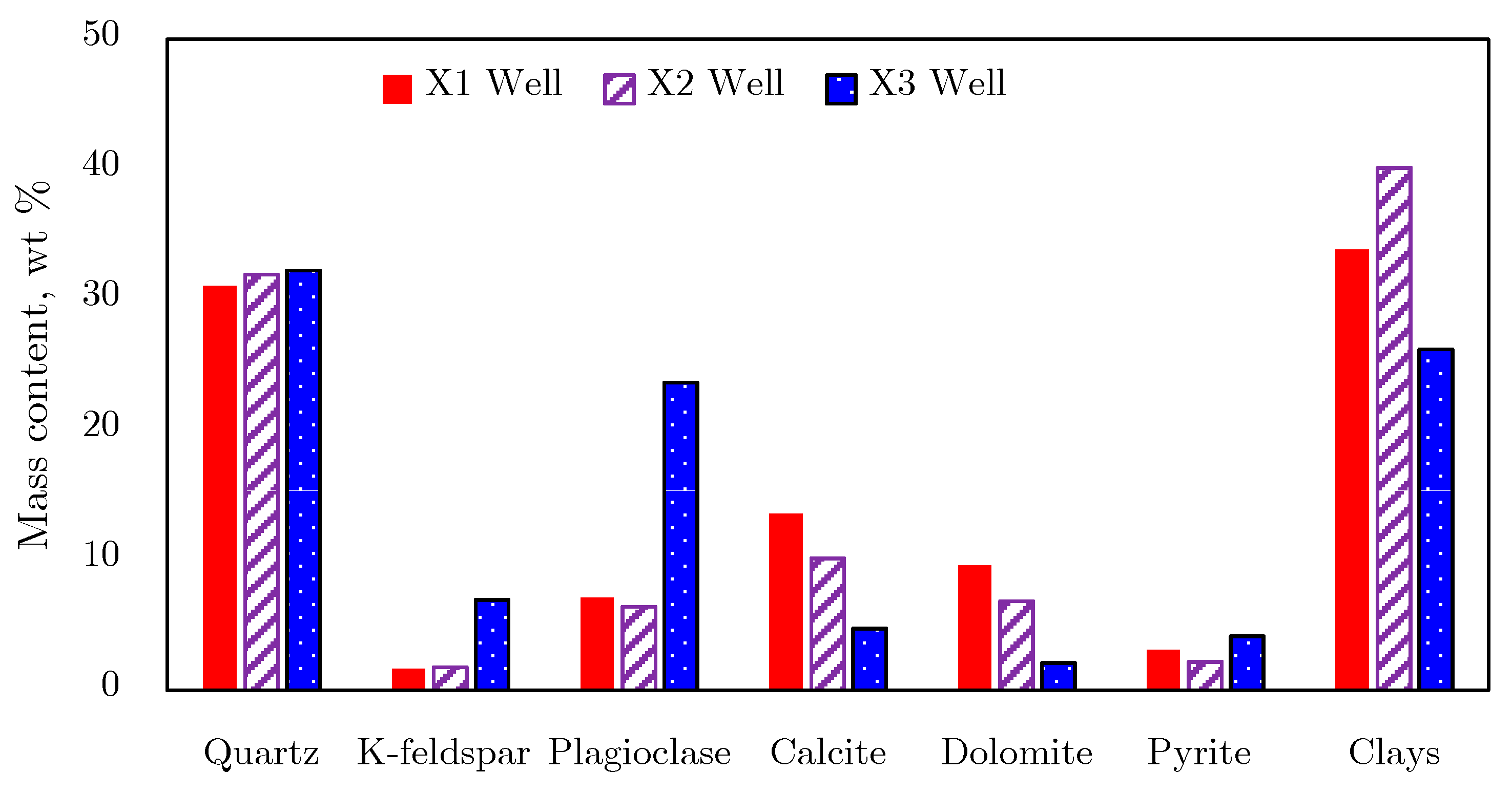
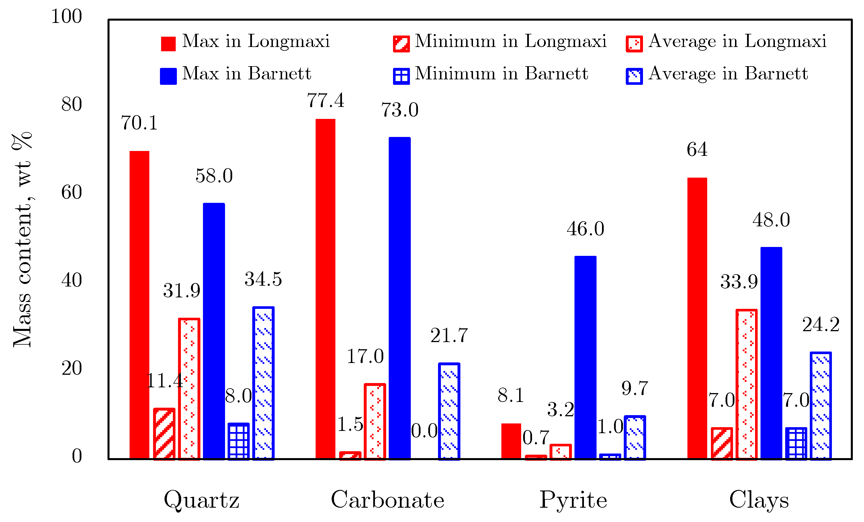
2.1.1. Mineral Composition
2.1.2. Organic Geochemical Characteristics of Shale
2.2. Porosity and Permeability Characterization
2.3. Pore Structure Division

| Major Classes | Subgroups | Types | |
|---|---|---|---|
| Fractures | Fractures | Tectonic extensional fractures (Figure 8a) [31] | |
| Tectonic shear fractures (Figure 8b) [31] | |||
| Interlayer bedding fractures (Figure 8c) | |||
| Rock convergent fractures (Figure 8d) | |||
| Abnormal pressure fractures (Figure 8e) | |||
| Matrix pores | Inorganic matrix pores | Intergranular pores | Intergranular pores among grains (Figure 8f) |
| Clay interslice pores (Figure 8g) | |||
| Intercrystalline pores (Figure 8h) | |||
| Marginal pores (Figure 8i) | |||
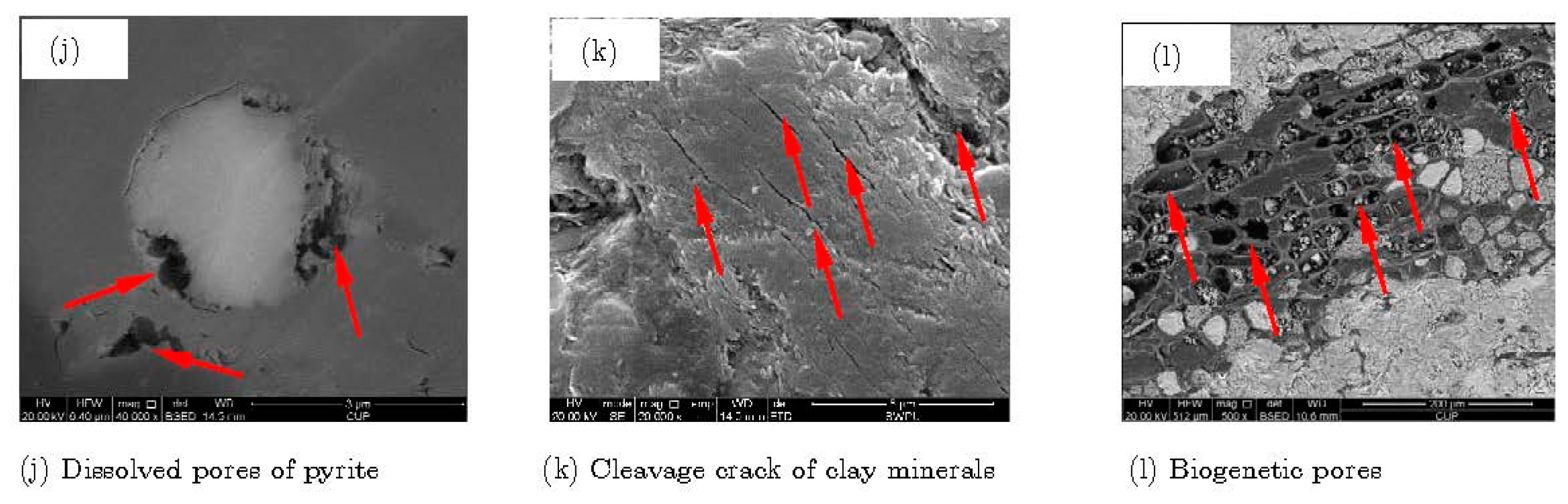
| Intragranular pores | Dissolved pores (Figure 8j) | ||
| Cleavage crack (Figure 8k) | |||
| Biological pores (Figure 8l) | |||
| Organic pores | |||
2.4. Pore Size Distribution and Influential Factors
2.4.1. Test Methods and Principles
N2 Adsorption Measurement
Mercury Injection Capillary Pressure
Nuclear Magnetic Resonance (NMR)
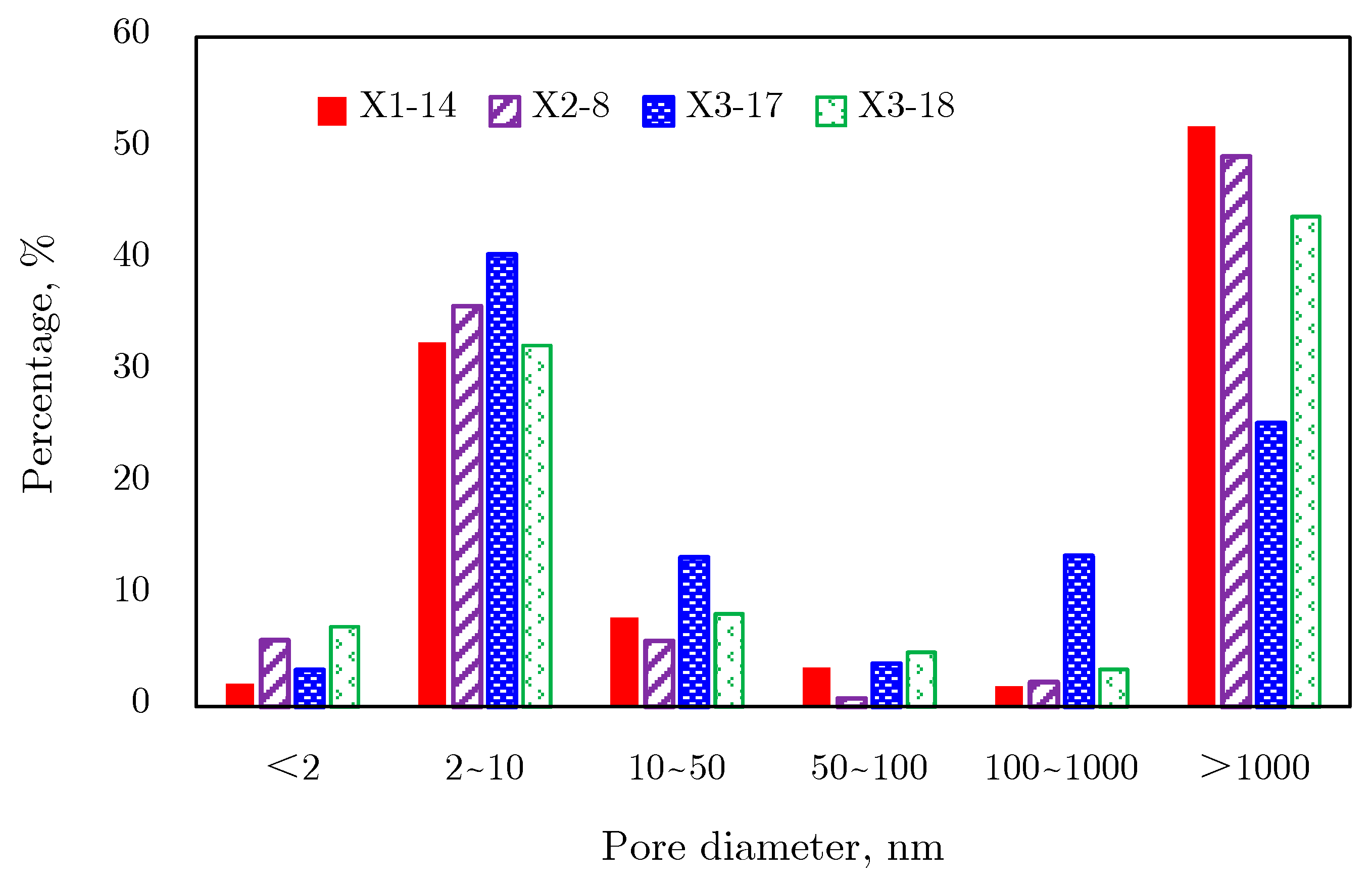
2.4.2. Pore Size Distribution
N2 Adsorption Results
Mercury Intrusion Results
Nuclear Magnetic Resonance Results
2.4.3. Comprehensive Analysis of Pore Size Distribution
2.5. Gas Composition and Origin
2.6. Shale Gas Occurrence Types
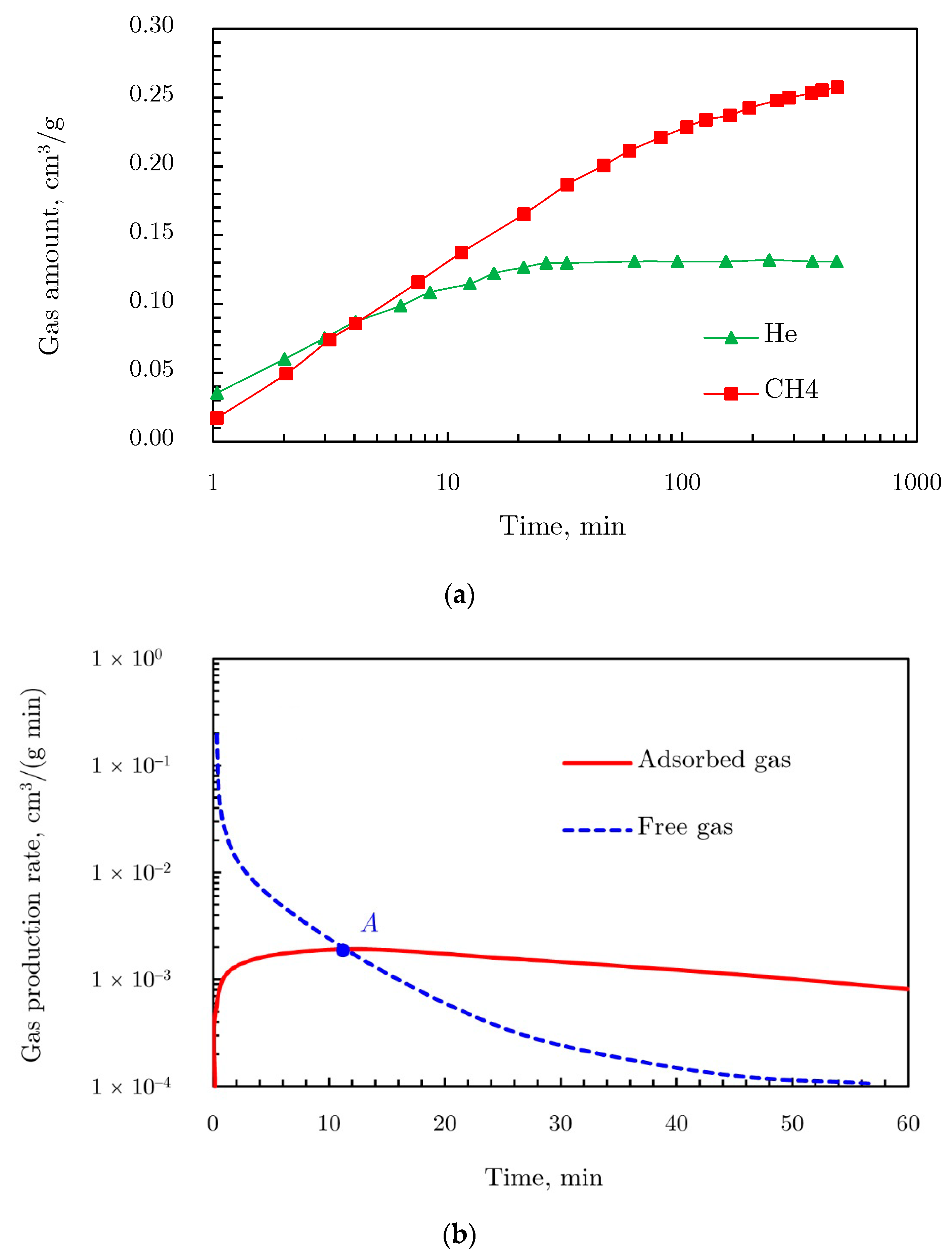
2.6.1. Free Gas Characterization
Semi-Empirical Formula
Empirical Formula
2.6.2. Adsorbed Gas
2.6.3. Dissolved Gas
3. Gas Adsorption and Desorption
3.1. Different Sorption Types and Models
3.1.1. Monolayer Adsorption Type
- (1)
- Langmuir model [68]: The Langmuir model was established by monolayer adsorption assumption. Due to its simplicity and accurate fitting to the experimental data, it is widely used to describe monolayer gas adsorption, which can be written as:where Ga is the absolute adsorbed gas amount; Gm is the maximum adsorbed capacity, p is the pressure, and b is the Langmuir sorption constant, which can be obtained by fitting the experimental or field test data.
- (2)
- Freundlich model [69]: With pressure decreasing, the Langmuir equation of Equation (10) approaches the Henry’s law of Equation (9). Therefore, the Henry’s law can describe low-pressure sorption behaviors, since any sorption isotherm satisfies the linear relationship between adsorption amount and pressure at low pressure. To broaden the application range of the Henry’s law into high-pressure areas, an exponential empirical formulation, namely the Freundlich model, was used:where kf is related to the adsorption interaction and adsorption amount; nf is a constant usually between 2 and 3, reflecting the intensity of adsorption. The values of both kf and nf depend on the type of adsorbent and adsorbate as well as the temperature.
- (3)
- Langmuir-Freundlich model: To modify the assumption of uniform adsorption sites in the Langmuir model, the Freundlich equation and the Langmuir equation were coupled to form a new adsorption model, namely the Langmuir‒Freundlich model, which is:where l reflects the heterogeneity of adsorbents, l ≤ 1. The smaller the value of l, the stronger the heterogeneity of the adsorbent. If an adsorbent possesses an ideal surface, l tends to be 1 and the Langmuir‒Freundlich equation is equivalent to the Langmuir equation.
- (4)
- Toth model [69]: To improve the fitting capacity of the Langmuir model, the Toth model was proposed:where t is a constant related to the adsorbent properties.
3.1.2. Multilayer Sorption Type
- (1)
- Two-parameter BET model [32]: Multilayer adsorption can be modeled by the BET sorption theory, which assumes that gas molecules can adsorb on a solid surface by infinite layers and no interaction exists between contiguous layers. In other words, any monolayer obeys the Langmuir adsorption theory in the BET model, which can be expressed as follows:where Gm is the maximum monolayer adsorption amount, ps is the saturated vapor pressure, and Cb is the dimensionless constant controlling the time of multilayer adsorption.
- (2)
3.1.3. Micropore Volume Filling
Dubinin–Radushkevich and Dubinin‒Astakhov Models
Calculation of Virtual Saturated Vapor Pressure
- (1)
- (2)
- (3)
- The third is the Antoine method [74]:Equation (20) is a three-parameter vapor pressure equation, where the extrapolation technique and saturated vapor pressure data under subcritical conditions are needed. For methane, three parameters can be obtained: BA = 8.784, CA = 933.51, and DA = −5.37, respectively [74]. Then, saturated vapor pressure could be calculated by Equation (20).
- (4)
- The fourth is the Astakhov method [72], the calculation results of which fit the experimental data well in the interval of ps from 0.1 MPa up to critical pressure pc [71]. Meanwhile, it should be noted that this method gives satisfactory results for temperatures exceeding the critical temperature by 50–100 K.where parameters cA and dA are determined by the gas critical point (Tc, pc) and boiling point (Tb, 101,325 Pa). For methane, cA = −1032.693 and dA = 6.945.
- (5)
- The Amankwah method [76] is an improved calculation method for the Dubinin method, which involves a parameter kA to account for interactions in an adsorbate‒adsorbent system:where kA is a parameter accounting for interactions in the adsorbate‒adsorbent systems.
- (6)
- The linearization of isotherm adsorption data is another processing method [77] to extend the D‒R and D‒A models into supercritical area. By transforming isotherms from Gex versus p space to ln[lnGex] − 1 versus lnp space, where Gex is the excess adsorption amount, a bunch of fitting straight lines could be obtained; they converge to a single point B, as shown in Figure 21. This merge point B is defined as the limiting state of the adsorbate, corresponding to the extreme condition of the adsorption potential field, where no more adsorptive molecules can enter the adsorbent micropores [77]. Therefore, the limiting pressure and limiting adsorption amount of the merge point correspond to the saturated vapor pressure and the saturated adsorption amount in the D‒R and D‒A models, respectively.
3.2. Sorption Study in Supercritical Area
3.2.1. Gibbs Excess Adsorption
3.2.2. Supercritical Adsorption Models
3.3. Adsorption/Absorption Models
- (1)
- Langmuir/Henry combination: In this model, gas adsorption is modeled by the Langmuir equation, and gas absorption is described by a term proportional to pressure, following Henry’s law. Here, the subcritical adsorption and absorption are described in terms of pressure, as in Equation (28), while supercritical adsorption and absorption are in terms of gas density [81] as in Equation (29):
- (2)
- Volume filling/Henry combination: Gas adsorption is described by the D‒R or D‒A model, and gas absorption is described by Henry’s law. For subcritical adsorption and absorption, this can be described in terms of pressure:For supercritical adsorption and absorption description in terms of gas density [81], this is:If gas pressure is adopted in a supercritical adsorption model [86], then the virtual saturated vapor pressure concept introduced in Section 3.1.3 needs to be employed, i.e.:
- (3)
- Swelling contribution: Dissolved gas usually swells the solid materials after absorption [83,85]. If the swelling contribution was equal to the condensed gas volume in adsorbents, Equations (28)–(32) need to be modified, because the swelling occupies space that would otherwise be taken up by gases [81]. The term (1 − ρg/ρad) needs to be multiplied by the absorption term. Taking the supercritical volume filling/Henry combination as an example, the model considering swelling contribution can be expressed as follows:Sakurovs et al. [81] compared the calculation results from the Langmuir model of Equation (27), the D‒R model of Equation (26), the Langmuir/Henry combination model of Equation (29), and the D‒R/Henry combination model of Equation (31) using CO2 and CH4 adsorption data, as shown in Figure 25a,b. The fitting effects of the Langmuir and the D‒R models are both poor, while the Langmuir/Henry or D‒R/Henry combination model has a much better effect. This means that the added term (kp) in adsorption models improves the fitting effect and reduces the calculated surface sorption capacity. The improvement of this term is greater in the D‒R model than in the Langmuir model, since the D‒R/Henry combination fits the measured sorption data better than the Langmuir/Henry combination. This suggest that the gas sorption mechanism in coal is more likely the volume filling, rather than monolayer coverage.
- (4)
- Bi-Langmuir adsorption model: Assuming absorption and swelling are related, Pini et al. [82] applied the Bi-Langmuir model [87] to describe the combination of adsorption and absorption, where linear superposition is adopted for each Langmuir adsorption term, i.e.:where the first term on the right side of the equation is the adsorption term, and the second term is the absorption term.
3.4. Physical Properties Calculation of Shale Gas
3.4.1. Bulk Gas Properties
Gas Density
- (1)
- Calculated by EOS: Generally, the bulk phase gas density can be calculated by the real gas EOS, as mentioned in Section 2.6.1. After calculation, we can also obtain the relationship between gas density and pressure by the nonlinear fitting technique, which expresses density in terms of pressure:where c0, c1, c2, and c3 are fitting parameters.
- (2)
- Measured by experiments: Bulk phase gas density can also by measured by experiments. Since analytical modeling is the main method introduced in this article, experimental measurement apparatus and procedures are not introduced.
Gas Viscosity
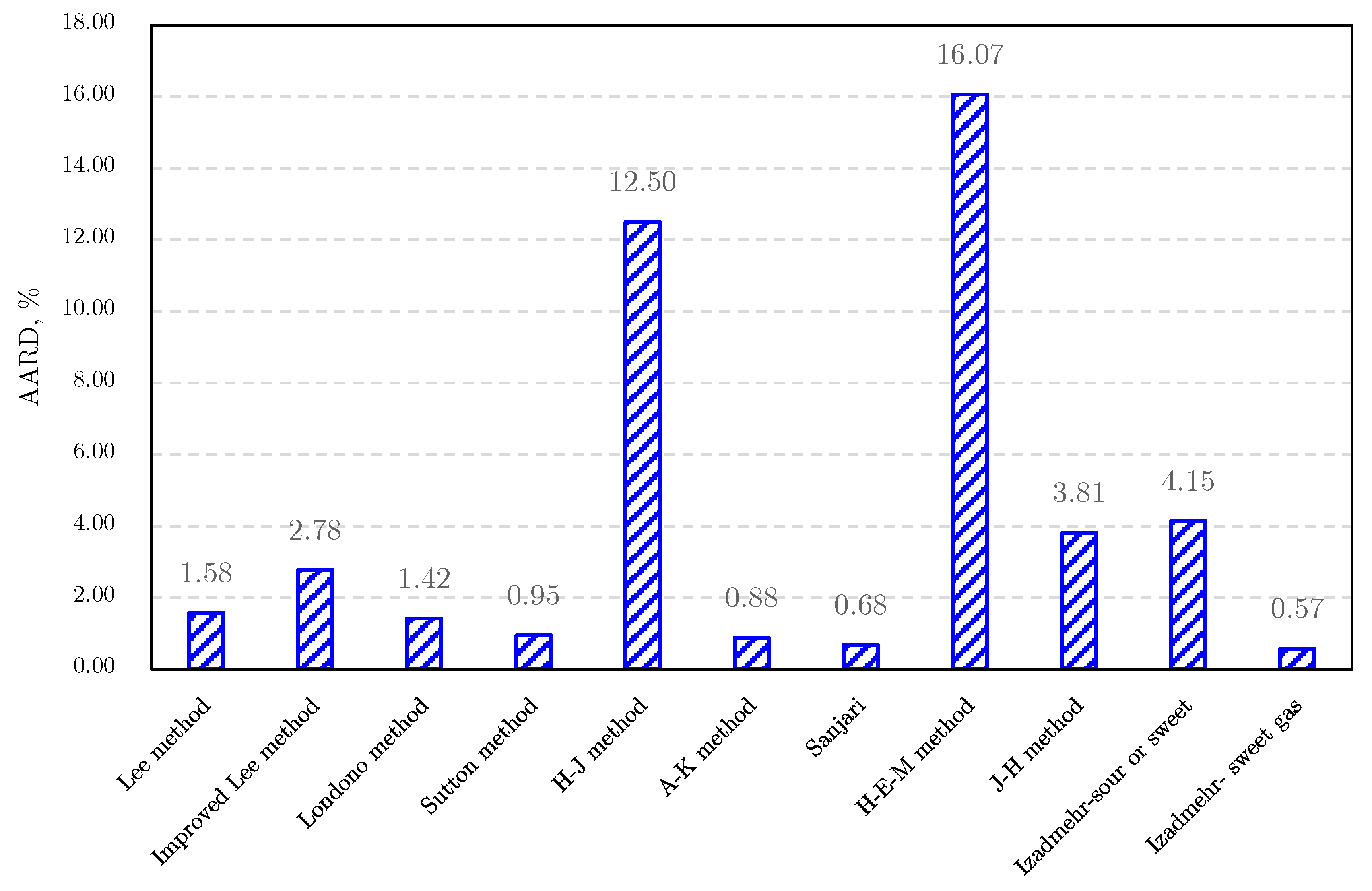
- (3)
- Londono method [92]
- (4)
- Sutton method [93]
- (5)
- Heidaryan and Jarrahian (H‒J) method [94].
- (6)
- Abooali‒Khamehchi (A‒K) method [95]
- (7)
- Heidaryan‒Moghadasi-Salarabadi (H‒M‒S) method [98]
- (8)
- Sanjari et al. method [99]
- (9)
- Heidaryan-Esmaeilzadeh-Moghadasi (H‒E‒M) method [96]
- (10)
- Jarrahian and Heidaryan Method [97]
- (11)
- Izadmehr method [100]
- (12)
- Low-pressure gas viscosity calculation
3.4.2. Adsorbed Gas Density
Empirical Formula
- (1)
- Dubinin method: Adsorbed gas density cannot be directly measured by experiments as the free gas density. As a result, many empirical formulations were proposed to approximately calculate its value. A temperature-independent formula was proposed by Dubinin [75,102] to approximate adsorbed gas density as follows:where b is the van der Waals covolume, representing the volume occupied by a single gas molecule.
- (2)
- (3)
- Ozawa method: Assuming adsorbed phase gas in a sort of superheated liquid state, Ozawa [75] calculated the density of adsorbed gas by the following equation [75]:where ρad is the adsorbed gas density, ρb is the liquid density at normal boiling point, T is the temperature, and Tb is the normal boiling point.
Experimental Method
4. Concluding Remarks
Author Contributions
Funding
Acknowledgments
Conflicts of Interest
References
- Shen, W.; Li, X.; Cihan, A.; Lu, X.; Liu, X. Experimental and numerical simulation of water adsorption and diffusion in shale gas reservoir rocks. Adv. Geo-Energy Res. 2019, 3, 165–174. [Google Scholar] [CrossRef]
- Bustin, R.M.; Bustin, A.M.M.; Cui, A.; Ross, D.; Pathi, V.M. Impact of Shale Properties on Pore Structure and Storage Characteristics. In Proceedings of the SPE Shale Gas Production Conference, Fort Worth, TX, USA, 16–18 November 2008; p. 28. [Google Scholar]
- Zhang, L.; Guo, J.; Tang, H. The Fundamental of Shale Gas Reservoir Development; Petroleum Industry Press: Beijing, China, 2014; (In Chinese). [Google Scholar] [CrossRef]
- Clarkson, C.R.; Jensen, J.L.; Chipperfield, S. Unconventional gas reservoir evaluation: What do we have to consider? J. Nat. Gas Sci. Eng. 2012, 8, 9–33. [Google Scholar] [CrossRef]
- Li, J.; Zhang, P.; Lu, S.; Chen, C.; Xue, H.; Wang, S.; Li, W. Scale-Dependent Nature of Porosity and Pore Size Distribution in Lacustrine Shales: An Investigation by BIB-SEM and X-Ray CT Methods. J. Earth Sci. 2018, 30, 823–833. [Google Scholar] [CrossRef]
- Daigle, H.; Johnson, A. Combining Mercury Intrusion and Nuclear Magnetic Resonance Measurements Using Percolation Theory. Transp. Porous Media 2015, 111, 669–679. [Google Scholar] [CrossRef]
- Deng, H.; Hu, X.; Li, H.A.; Luo, B.; Wang, W. Improved pore-structure characterization in shale formations with FESEM technique. J. Nat. Gas Sci. Eng. 2016, 35, 309–319. [Google Scholar] [CrossRef]
- Zhao, P.; Wang, Z.; Sun, Z.; Cai, J.; Wang, L. Investigation on the pore structure and multifractal characteristics of tight oil reservoirs using NMR measurements: Permian Lucaogou Formation in Jimusaer Sag, Junggar Basin. Mar. Pet. Geol. 2017, 86, 1067–1081. [Google Scholar] [CrossRef]
- Karimi, S.; Saidian, M.; Prasad, M.; Kazemi, H. Reservoir Rock Characterization Using Centrifuge and Nuclear Magnetic Resonance: A Laboratory Study of Middle Bakken Cores. In Proceedings of the SPE Annual Technical Conference and Exhibition, Houston, TX, USA, 28–30 September 2015; p. 18. [Google Scholar]
- Shao, D.; Zhang, T.; Ko, L.T.; Luo, H.; Zhang, D. Empirical plot of gas generation from oil-prone marine shales at different maturity stages and its application to assess gas preservation in organic-rich shale system. Mar. Pet. Geol. 2019, 102, 258–270. [Google Scholar] [CrossRef]
- Dai, J.; Zou, C.; Liao, S.; Dong, D.; Ni, Y.; Huang, J.; Wu, W.; Gong, D.; Huang, S.; Hu, G. Geochemistry of the extremely high thermal maturity Longmaxi shale gas, southern Sichuan Basin. Org. Geochem. 2014, 74, 3–12. [Google Scholar] [CrossRef]
- Yang, F.; Ning, Z.; Liu, H. Fractal characteristics of shales from a shale gas reservoir in the Sichuan Basin, China. Fuel 2014, 115, 378–384. [Google Scholar] [CrossRef]
- Zou, C.; Zhu, R.; Chen, Z.Q.; Ogg, J.G.; Wu, S.; Dong, D.; Qin, Z.; Wang, Y.; Wang, L.; Lin, S.; et al. Organic-matter-rich shales of China. Earth-Sci. Rev. 2019, 189, 51–78. [Google Scholar] [CrossRef]
- Fan, C.; Li, H.; Qin, Q.; He, S.; Zhong, C. Geological conditions and exploration potential of shale gas reservoir in Wufeng and Longmaxi Formation of southeastern Sichuan Basin, China. J. Pet. Sci. Eng. 2020, 191, 107138. [Google Scholar] [CrossRef]
- Montgomery, S.L.; Jarvie, D.M.; Bowker, K.A.; Pollastro, R.M. Mississippian Barnett Shale, Fort Worth basin, north-central Texas: Gas-shale play with multi–trillion cubic foot potential: Reply. AAPG Bull. 2006, 90, 967–969. [Google Scholar] [CrossRef]
- Loucks, R.G.; Ruppel, S.C. Mississippian Barnett Shale: Lithofacies and depositional setting of a deep-water shale-gas succession in the Fort Worth Basin, Texas. AAPG Bull. 2007, 91, 579–601. [Google Scholar] [CrossRef]
- Zou, C.; Dong, D.; Wang, S.; Li, J.; Li, X.; Wang, Y.; Li, D.; Cheng, K. Geological characteristics, formation mechanism and resource potential of shale gas in China (in Chinese with English abstract). Pet. Explor. Dev. 2010, 37, 641–653. [Google Scholar] [CrossRef]
- Bowker, K.A. Barnett Shale gas production, Fort Worth Basin: Issues and discussion. AAPG Bull. 2007, 91, 523–533. [Google Scholar] [CrossRef]
- Curtis, J.B. Fractured shale-gas systems. AAPG Bull. 2002, 86, 1921–1938. [Google Scholar]
- Jarvie, D.M.; Hill, R.J.; Ruble, T.E.; Pollastro, R.M. Unconventional shale-gas systems: The Mississippian Barnett Shale of north-central Texas as one model for thermogenic shale-gas assessment. AAPG Bull. 2007, 91, 475–499. [Google Scholar] [CrossRef]
- Jarvie, D.M.; Hill, R.; Pollastro, R.; Wavrek, D.; Claxton, B.; Tobey, M. Evaluation of unconventional natural gas prospects: The Barnett Shale fractured shale gas model. In Proceedings of the European Association of International Organic Geochemists Meeting, Kraków, Poland, 8–12 September 2003. [Google Scholar]
- Martineau, D.F. History of the Newark East field and the Barnett Shale as a gas reservoir. AAPG Bull. 2007, 91, 399–403. [Google Scholar] [CrossRef]
- Pollastro, R.M.; Jarvie, D.M.; Hill, R.J.; Adams, C.W. Geologic framework of the Mississippian Barnett Shale, Barnett-Paleozoic total petroleum system, Bend arch-Fort Worth Basin, Texas. AAPG Bull. 2007, 91, 405–436. [Google Scholar] [CrossRef]
- Welte, D.H.; Tissot, B.P. Petroleum Formation and Occurrence; Springer: Berlin/Heidelberg, Germany, 1984. [Google Scholar]
- David, G.; Charles, R.N. Gas productive fractured shales: An overview and update. Gas Tips 2000, 6, 4–13. [Google Scholar] [CrossRef]
- Warlick, D. Gas shale and CBM development in North America. Oil Gas Financ. J. 2006, 3, 1–5. [Google Scholar]
- Zhang, L.H.; Shan, B.C.; Zhao, Y.L.; Guo, Z.L. Review of micro seepage mechanisms in shale gas reservoirs. Int. J. Heat Mass Transfer 2019, 139, 144–179. [Google Scholar] [CrossRef]
- Loucks, R.G.; Reed, R.M.; Ruppel, S.C.; Jarvie, D.M. Morphology, Genesis, and Distribution of Nanometer-Scale Pores in Siliceous Mudstones of the Mississippian Barnett Shale. J. Sediment. Res. 2009, 79, 848–861. [Google Scholar] [CrossRef]
- Slatt, R.M.; O’Brien, N.R. Pore types in the Barnett and Woodford gas shales: Contribution to understanding gas storage and migration pathways in fine-grained rocks. AAPG Bull. 2011, 95, 2017–2030. [Google Scholar] [CrossRef]
- Loucks, R.G.; Reed, R.M.; Ruppel, S.C.; Hammes, U. Spectrum of pore types and networks in mudrocks and a descriptive classification for matrix-related mudrock pores. AAPG Bull. 2012, 96, 1071–1098. [Google Scholar] [CrossRef]
- Long, P.; Zhang, J.; Tang, X.; Nie, H.; Liu, Z.; Han, S.; Zhu, L. Feature of muddy shale fissure and its effect for shale gas exploration and development (in Chinese with English abstract). Nat. Gas Geosci. 2011, 22, 525–532. [Google Scholar]
- Brunauer, S.; Emmett, P.H.; Teller, E. Adsorption of gases in multimolecular layers. J. Am. Chem. Soc. 1938, 60, 309–319. [Google Scholar] [CrossRef]
- Chen, J.; Wang, F.C.; Liu, H.; Wu, H.A. Molecular mechanism of adsorption/desorption hysteresis:dynamics of shale gas in nanopores. Sci. China (Phys. Mech. Astron. ) 2017, 60, 014611. [Google Scholar] [CrossRef]
- Barrett, E.P.; Joyner, L.G.; Halenda, P.P. The determination of pore volume and area distributions in porous substances. I. Computations from nitrogen isotherms. J. Am. Chem. Soc. 1951, 73, 373–380. [Google Scholar] [CrossRef]
- Washburn, E.W. The Dynamics of Capillary Flow. Phys. Rev. 1921, 17, 273–283. [Google Scholar] [CrossRef]
- Chen, Y.; Zhang, L.; Li, J. Study of Pore Structure of Gas Shale with Low-Field NMR: Examples from the Longmaxi Formation, Southern Sichuan Basin, China. Soc. Pet. Eng. 2015. [Google Scholar] [CrossRef]
- Milkov, A.V.; Faiz, M.; Etiope, G. Geochemistry of shale gases from around the world: Composition, origins, isotope reversals and rollovers, and implications for the exploration of shale plays. Org. Geochem. 2020, 143, 103997. [Google Scholar] [CrossRef]
- Zhang, L.; Shan, B.; Zhao, Y.; Tang, H. Comprehensive Seepage Simulation of Fluid Flow in Multi-scaled Shale Gas Reservoirs. Transp. Porous Media 2017, 121, 263–288. [Google Scholar] [CrossRef]
- Cai, J.; Lin, D.; Singh, H.; Zhou, S.; Meng, Q.; Zhang, Q. A simple permeability model for shale gas and key insights on relative importance of various transport mechanisms. Fuel 2019, 252, 210–219. [Google Scholar] [CrossRef]
- Javadpour, F. Nanopores and Apparent Permeability of Gas Flow in Mudrocks (Shales and Siltstone). J. Can. Petrol. Technol. 2009, 48, 16–21. [Google Scholar] [CrossRef]
- Zhang, L.; Shan, B.; Zhao, Y.; Du, J.; Chen, J.; Tao, X. Gas Transport Model in Organic Shale Nanopores Considering Langmuir Slip Conditions and Diffusion: Pore Confinement, Real Gas, and Geomechanical Effects. Energies 2018, 11, 223. [Google Scholar] [CrossRef]
- Zhang, T.; Li, Y.; Sun, S. Phase equilibrium calculations in shale gas reservoirs. Capillarity 2019, 2, 8–16. [Google Scholar] [CrossRef]
- Shen, W.; Song, F.; Hu, X.; Zhu, G.; Zhu, W. Experimental study on flow characteristics of gas transport in micro- and nanoscale pores. Sci. Rep. 2019, 9, 10196. [Google Scholar] [CrossRef]
- Li, S. Natural Gas Engineering; Petroleum Industry Press: Beijing, China, 2008. [Google Scholar]
- Zhang, R.H.; Zhang, L.H.; Tang, H.Y.; Chen, S.N.; Zhao, Y.L.; Wu, J.F.; Wang, K.R. A Simulator for Production Prediction of Multistage Fractured Horizontal Well in Shale Gas Reservoir Considering Complex Fracture Geometry. J. Nat. Gas Sci. Eng. 2019, 67, 14–29. [Google Scholar] [CrossRef]
- Zhang, R.H.; Zhang, L.H.; Wang, R.H.; Zhao, Y.L.; Zhang, D.L. Research on transient flow theory of a multiple fractured horizontal well in a composite shale gas reservoir based on the finite-element method. J. Nat. Gas Sci. Eng. 2016, 33, 587–598. [Google Scholar] [CrossRef]
- Wang, Y.; Shahvali, M. Discrete fracture modeling using Centroidal Voronoi grid for simulation of shale gas plays with coupled nonlinear physics. Fuel 2016, 163, 65–73. [Google Scholar] [CrossRef]
- Deliang, Z.; Liehui, Z.; Jingjing, G.; Yuhui, Z.; Yulong, Z. Research on the production performance of multistage fractured horizontal well in shale gas reservoir. J. Nat. Gas Sci. Eng. 2015, 26, 279–289. [Google Scholar] [CrossRef]
- Mengal, S.A.; Wattenbarger, R.A. Accounting For Adsorbed Gas in Shale Gas Reservoirs. In Proceedings of the SPE Middle East Oil and Gas Show and Conference, Manama, Bahrain, 25–28 September 2011; p. 15. [Google Scholar]
- Wang, L.; Wang, S.; Zhang, R.; Wang, C.; Xiong, Y.; Zheng, X.; Li, S.; Jin, K.; Rui, Z. Review of multi-scale and multi-physical simulation technologies for shale and tight gas reservoirs. J. Nat. Gas Sci. Eng. 2017, 37, 560–578. [Google Scholar] [CrossRef]
- Taotao, C.; Zhiguang, S.; Sibo, W.; Jia, X. A comparative study of the specific surface area and pore structure of different shales and their kerogens. Sci. China Earth Sci. 2015, 58, 510–522. [Google Scholar]
- Wang, F.P.; Reed, R.M. Pore Networks and Fluid Flow in Gas Shales. In Proceedings of the SPE Annual Technical Conference and Exhibition, New Orleans, LA, USA, 4–7 October 2009; p. 8. [Google Scholar]
- Zhao, Y.; Shan, B.; Zhang, L.; Liu, Q. Seepage flow behaviors of multi-stage fractured horizontal wells in arbitrary shaped shale gas reservoirs. J. Geophys. Eng. 2016, 13, 674–689. [Google Scholar] [CrossRef]
- Fathi, E.; Akkutlu, I.Y. Multi-component gas transport and adsorption effects during CO2 injection and enhanced shale gas recovery. Int. J. Coal Geol. 2014, 123, 52–61. [Google Scholar] [CrossRef]
- Cai, J.; Lin, D.; Singh, H.; Wei, W.; Zhou, S. Shale gas transport model in 3D fractal porous media with variable pore sizes. Mar. Petrol. Geol. 2018, 98, 437–447. [Google Scholar] [CrossRef]
- Kim, T.H.; Cho, J.; Lee, K.S. Evaluation of CO2 injection in shale gas reservoirs with multi-component transport and geomechanical effects. Appl. Energy 2017, 190, 1195–1206. [Google Scholar] [CrossRef]
- Yin, Y.; Qu, Z.G.; Zhang, J.F. Multiple diffusion mechanisms of shale gas in nanoporous organic matter predicted by the local diffusivity lattice Boltzmann model. Int. J. Heat Mass Transfer 2019, 143, 118571. [Google Scholar] [CrossRef]
- Zhang, T.; Sun, S. A coupled Lattice Boltzmann approach to simulate gas flow and transport in shale reservoirs with dynamic sorption. Fuel 2019, 246, 196–203. [Google Scholar] [CrossRef]
- Javadpour, F.; Fisher, D.; Unsworth, M. Nanoscale Gas Flow in Shale Gas Sediments. J. Can. Petrol. Technol. 2007, 46. [Google Scholar] [CrossRef]
- Wang, J.; Yang, Z.; Dong, M.; Gong, H.; Sang, Q.; Li, Y. Experimental and Numerical Investigation of Dynamic Gas Adsorption/Desorption Diffusion Process in Shale. Energy Fuels 2016, 30, 10080–10091. [Google Scholar] [CrossRef]
- Tang, X.; Ripepi, N.; Stadie, N.P.; Yu, L.; Hall, M.R. A dual-site Langmuir equation for accurate estimation of high pressure deep shale gas resources. Fuel 2016, 185, 10–17. [Google Scholar] [CrossRef]
- Lopez, B.; Aguilera, R. Sorption-Dependent Permeability of Shales. In Proceedings of the Spe/csur Unconventional Resources Conference, Calgary, AB, Canada, 20–22 October 2015. [Google Scholar]
- Ross, D.J.K.; Marc Bustin, R. The importance of shale composition and pore structure upon gas storage potential of shale gas reservoirs. Mar. Pet. Geol. 2009, 26, 916–927. [Google Scholar] [CrossRef]
- Zhang, L.; Li, J.; Jia, D.U.; Zhao, Y.; Xie, C.; Tao, Z. Study on the Adsorption Phenomenon in Shale with the Combination of Molecular Dynamic Simulation and Fractal Analysis. Fractals 2018, 26, 1840004. [Google Scholar] [CrossRef]
- Zhang, L.; Chen, Z.; Zhao, Y. Well Production Performance Analysis for Shale Gas Reservoirs; Candice Janco: Amsterdam, The Netherlands, 2019; Volume 66. [Google Scholar]
- Yin, Y.; Qu, Z.G.; Zhang, J.F. An analytical model for shale gas transport in kerogen nanopores coupled with real gas effect and surface diffusion. Fuel 2017, 210, 569–577. [Google Scholar] [CrossRef]
- Zhou, S.; Wang, H.; Xue, H.; Guo, W.; Li, X. Discussion on the Supercritical Adsorption Mechanism of Shale Gas Based on Ono-Kondo Lattice Model (in Chinese with English abstract). Earth Sci. 2017, 42, 1421–1430. [Google Scholar]
- Langmuir, I. The Adsorption of Gases on Plane Surfaces of Glass, Mica and Platinum. J. Am. Chem. Soc. 1918, 40, 1361–1403. [Google Scholar] [CrossRef]
- Bae, J.-S.; Bhatia, S.K. High-pressure adsorption of methane and carbon dioxide on coal. Energy Fuels 2006, 20, 2599–2607. [Google Scholar] [CrossRef]
- Wang, Y.; Zhu, Y.; Liu, S.; Zhang, R. Methane adsorption measurements and modeling for organic-rich marine shale samples. Fuel 2016, 172, 301–309. [Google Scholar] [CrossRef]
- Dubinin, M.M. Progress in Membrane and Surface Science; Cadenhead, D.A., Ed.; Academic Press: New York, NY, USA, 1975; Volume 9, pp. 1–70. Available online: https://scholar.google.com/scholar?q=M.+M.+Dubinin,+Progress+in+Surface+and+Membrane+Science,+Academic+Press,+New+York,+1975&hl=zh-CN&as_sdt=0,5 (accessed on 4 April 2020).
- Yang, F.; Xie, C.; Xu, S.; Ning, Z.; Krooss, B.M. Supercritical Methane Sorption on Organic-Rich Shales over a Wide Temperature Range. Energy Fuels 2017, 31, 13427–13438. [Google Scholar] [CrossRef]
- Manes, M.; Hofer, L.J.E. Application of the Polanyi adsorption potential theory to adsorption from solution on activated carbon. J. Phys. Chem. 1969, 73, 584–590. [Google Scholar] [CrossRef]
- Agarwal, R.K.; Amankwah, K.A.G.; Schwarz, J.A. Analysis of adsorption entropies of high pressure gas adsorption data on activated carbon. Carbon 1990, 28, 169–174. [Google Scholar] [CrossRef]
- Wakasugi, Y.; Ozawa, S.; Ogino, Y. Physical Adsorption of Gases at High Pressure (IV). J. Colloid Interface Sci. 1981, 79, 399–409. [Google Scholar] [CrossRef]
- Amankwah, K.A.G.; Schwarz, J.A. A Modified Approach for Estimating Pseudo Vapor Pressures in the Application of the Dubinin-Astakhov Equation. Carbon 1995, 33, 1313–1319. [Google Scholar] [CrossRef]
- Zhou, L.; Zhou, Y.P. Linearization of adsorption isotherms for high-pressure applications - Argon and methane onto graphitized carbon black. Chem. Eng. Sci. 1998, 53, 2531–2536. [Google Scholar] [CrossRef]
- Zhang, T.; Ellis, G.S.; Ruppel, S.C.; Milliken, K.; Yang, R. Effect of organic-matter type and thermal maturity on methane adsorption in shale-gas systems. Org. Geochem. 2012, 47, 120–131. [Google Scholar] [CrossRef]
- Zhou, S.; Ning, Y.; Wang, H.; Liu, H.; Xue, H. Investigation of methane adsorption mechanism on Longmaxi shale by combining the micropore filling and monolayer coverage theories. Adv.Geo-Energy Res. 2018, 2, 269–281. [Google Scholar] [CrossRef]
- Moellmer, J.; Moeller, A.; Dreisbach, F.; Glaeser, R.; Staudt, R. High pressure adsorption of hydrogen, nitrogen, carbon dioxide and methane on the metal–organic framework HKUST-1. Microporous Mesoporous Mater. 2011, 138, 140–148. [Google Scholar] [CrossRef]
- Sakurovs, R.; Day, S.; Weir, S.; Duffy, G. Application of a Modified Dubinin—Radushkevich Equation to Adsorption of Gases by Coals under Supercritical Conditions. Energy Fuels 2007, 21, 992–997. [Google Scholar] [CrossRef]
- Pini, R.; Ottiger, S.; Burlini, L.; Storti, G.; Mazzotti, M. Sorption of carbon dioxide, methane and nitrogen in dry coals at high pressure and moderate temperature. Int. J. Greenh. Gas Control 2010, 4, 90–101. [Google Scholar] [CrossRef]
- Reucroft, P.J.; Patel, K.B. Surface area and swellability of coal. Fuel 1983, 62, 279–284. [Google Scholar] [CrossRef]
- Sato, Y.; Takikawa, T.; Yamane, M.; Takishima, S.; Masuoka, H. Solubility of carbon dioxide in PPO and PPO/PS blends. Fluid Phase Equilib. 2002, 194, 847–858. [Google Scholar] [CrossRef]
- Larsen, J.W. The effects of dissolved CO2 on coal structure and properties. Int. J. Coal Geol. 2004, 57, 63–70. [Google Scholar] [CrossRef]
- Ozdemir, E.; Morsi, B.I.; Schroeder, K. CO2 adsorption capacity of argonne premium coals. Fuel 2004, 83, 1085–1094. [Google Scholar] [CrossRef]
- Fornstedt, T.; Zhong, G.; Bensetiti, Z.; Guiochon, G. Experimental and theoretical study of the adsorption behavior and mass transfer kinetics of propranolol enantiomers on cellulase protein as the selector. Anal. Chem. 1996, 68, 2370–2378. [Google Scholar] [CrossRef] [PubMed]
- Lee, A.L.; Gonzalez, M.H.; Eakin, B.E. The Viscosity of Natural Gases. J. Pet. Technol. 1966, 18, 997–1000. [Google Scholar] [CrossRef]
- Lee, A.; Starling, K.; Dolan, J.; Ellington, R. Viscosity correlation for light hydrocarbon systems. AlChE J. 1964, 10, 694–697. [Google Scholar] [CrossRef]
- McCain, W.D., Jr. Reservoir-Fluid Property Correlations-State of the Art. SPE Reserv. Eng. 1991, 6, 266–277. [Google Scholar] [CrossRef]
- Naraghi, M.E.; Javadpour, F. A stochastic permeability model for the shale-gas systems. Int. J. Coal Geol. 2015, 140, 111–124. [Google Scholar] [CrossRef]
- Londono, F.E.; Archer, R.A.; Blasingame, T.A. Correlations for Hydrocarbon Gas Viscosity and Gas Density—Validation and Correlation of Behavior Using a Large-Scale Database. SPE Reserv. Eval. Eng. 2005, 8, 561–572. [Google Scholar] [CrossRef]
- Sutton, R.P. Fundamental PVT Calculations for Associated and Gas/Condensate Natural-Gas Systems. SPE Reserv. Eval. Eng. 2007, 10, 270–284. [Google Scholar] [CrossRef]
- Heidaryan, E.; Jarrahian, A. Natural gas viscosity estimation using density based models. Can. J. Chem. Eng. 2013, 91. [Google Scholar] [CrossRef]
- Abooali, D.; Khamehchi, E. Estimation of dynamic viscosity of natural gas based on genetic programming methodology. J. Nat. Gas Sci. Eng. 2014, 21, 1025–1031. [Google Scholar] [CrossRef]
- Heidaryan, E.; Esmaeilzadeh, F.; Moghadasi, J. Natural gas viscosity estimation through corresponding states based models. Fluid Phase Equilib. 2013, 354, 80–88. [Google Scholar] [CrossRef]
- Jarrahian, A.; Heidaryan, E. A simple correlation to estimate natural gas viscosity. J. Nat. Gas Sci. Eng. 2014, 20, 50–57. [Google Scholar] [CrossRef]
- Heidaryan, E.; Moghadasi, J.; Salarabadi, A. A new and reliable model for predicting methane viscosity at high pressures and high temperatures. J. Nat. Gas Chem. 2010, 19, 552–556. [Google Scholar] [CrossRef]
- Sanjari, E.; Lay, E.N. An accurate empirical correlation for predicting natural gas viscosity. J. Nat. Gas Chem. 2011, 20, 654–658. [Google Scholar] [CrossRef]
- Izadmehr, M.; Shams, R.; Ghazanfari, M.H. New correlations for predicting pure and impure natural gas viscosity. J. Nat. Gas Sci. Eng. 2016, 30, 364–378. [Google Scholar] [CrossRef]
- Hurly, J.J.; Gillis, K.A.; Mehl, J.B.; Moldover, M.R. The Viscosity of Seven Gases Measured with a Greenspan Viscometer. Int. J. Thermophys. 2003, 24, 1441–1474. [Google Scholar] [CrossRef]
- Dubinin, M. The potential theory of adsorption of gases and vapors for adsorbents with energetically nonuniform surfaces. Chem. Rev. 1960, 60, 235–241. [Google Scholar] [CrossRef]
- Li, J.; Chen, Z.; Wu, K.; Wang, K.; Luo, J.; Feng, D.; Qu, S.; Li, X. A multi-site model to determine supercritical methane adsorption in energetically heterogeneous shales. Chem. Eng. J. 2018, 349, 438–455. [Google Scholar] [CrossRef]
- Sudibandriyo, M.; Pan, Z.; Fitzgerald, J.E.; Robinson, R.L.; Gasem, K.A.M. Adsorption of Methane, Nitrogen, Carbon Dioxide, and Their Binary Mixtures on Dry Activated Carbon at 318.2 K and Pressures up to 13.6 MPa. Langmuir 2003, 19, 5323–5331. [Google Scholar] [CrossRef]


| Maturity of OM | Maturity Class | Hydrocarbon Generating Stage |
|---|---|---|
| Ro < 0.5% | Immaturity | Biochemical gas-genous stage |
| 0.5% < Ro < 1.3% | Maturity | Thermal catalytic oil and gas genous stage |
| 1.3% < Ro < 2.0% | High maturity | Thermal cracking condensate gas-genous stage |
| Ro > 2.0% | Overmaturity | Deep high temperature gas-geneous stage |
| Properties | Woodford | Marcellus | Fayetteville | Haynesville | Barnett | Antrim | New Albany | Lewis | Ohio |
|---|---|---|---|---|---|---|---|---|---|
| Permeability, mD | - | - | - | - | 0.01 | <0.1 | <0.1 | <0.1 | <0.1 |
| Total porosity, % | 3‒9 | 10 | 2‒8 | 8‒9 | 4‒5 | 9 | 10‒14 | 3‒5.5 | 4.7 |
| Logging porosity, % | 3‒6.5 | 5.5‒7.5 | 4‒12 | 8‒10 | 6.5‒8.5 | - | - | - | - |
| Gas porosity, % | - | - | - | 6‒7.5 | 2.5 | 4 | 5 | 1‒3.5 | 2 |
| Water porosity, % | - | - | - | - | 1.9 | 4 | 4‒8 | 1‒2 | 2.5‒3 |
| Water-filled porosity, % | 10 | 12‒35 | 15‒35 | 15‒20 | 25 | - | - | - | - |
| Types | Zc | Pros | Cons |
|---|---|---|---|
| vdW | 0.375 | Simple; basis of other EOS | Low accuracy; seldom practical for application |
| RK | 0.333 | Practical; accurate to calculate gas phase volume | Failed to calculate liquid volume accurately |
| SRK | 0.333 | Calculate gas and liquid phase equilibrium; widely used | The error is large when calculating liquid volume |
| PR | 0.307 | Higher accuracy than SRK to calculate liquid volume | Zc is slightly bigger than the practical value |
| Virial | Able to describe viscosity, sound velocity, and heat capacity of gases | Failed to calculate liquid volume; inaccurate at high pressure |
| Coefficients | i = 0 | i = 1 | i = 2 |
|---|---|---|---|
| ali | 0.953363 | −1.07384 | 0.00131729 |
| bli | −0.971028 | 11.2077 | 0.09013 |
| cli | 1.01803 | 4.98986 | 0.302737 |
| dli | −0.990531 | 4.17585 | −0.63662 |
| eli | 1 | −3.19646 | 3.90961 |
| fli | −1.00364 | −0.181633 | −7.79089 |
| gli | 0.99808 | −1.62108 | 0.000634836 |
| hli | −1.00103 | 0.676875 | 4.62481 |
| Coefficient | Tuned Coefficient |
|---|---|
| H1 | −336.6309996192 |
| H2 | 1.432588837697 |
| H3 | 113,908.9211105 |
| H4 | −380,054.8489939 |
| H5 | 384,369,898.3053 |
| H6 | 4.098692867002 |
| H7 | −0.003307304447043 |
| H8 | −0.004252150356903 |
| H9 | 718.2941490688 |
| H10 | 1.658818877773 |
| H11 | −0.00580479565535 |
| H12 | −0.001129165058823 |
| H13 | −204.6192651917 |
| Coefficient | For ppr ≤ 3 | For ppr > 3 |
|---|---|---|
| Ae1 | −0.574429785927299 | −1.61486373676777 |
| Ae2 | −0.161401455390735 | 0.393317983084269 |
| Ae3 | 0.111211457326131 | 0.273470537671412 |
| Ae4 | 0.0300553354088043 | 0.00142823962661707 |
| Ae5 | 5.56157730361211 | −0.779279490434404 |
| Ae6 | −4.08580223632285 | 0.142553527534496 |
| Ae7 | −1.08843921447191 | 0.581332491577921 |
| Ae8 | 0.694563966721831 | 0.00329912709369652 |
| Ae9 | 0.13871744921249 | 0.0243974777653492 |
| Ae10 | −0.0420997501646278 | −0.0000632194669476397 |
| Coefficient | Sour/Sweet Natural Gas Equation (70) | Sweet Natural Gas Equation (71) |
|---|---|---|
| aiz | 0.033359716350877 | 0.0085050748654501 |
| biz | −0.00303297726852698 | −0.00104065426590739 |
| ciz | −0.0514170415427857 | −0.00217777225933512 |
| diz | 0.0000187555872613017 | −0.000510724061609292 |
| eiz | 0.0233088265671431 | 0.00595154429253907 |
| fiz | 0.00880957960915389 | −0.000548942531453252 |
Publisher’s Note: MDPI stays neutral with regard to jurisdictional claims in published maps and institutional affiliations. |
© 2020 by the authors. Licensee MDPI, Basel, Switzerland. This article is an open access article distributed under the terms and conditions of the Creative Commons Attribution (CC BY) license (http://creativecommons.org/licenses/by/4.0/).
Share and Cite
Zhang, B.; Shan, B.; Zhao, Y.; Zhang, L. Review of Formation and Gas Characteristics in Shale Gas Reservoirs. Energies 2020, 13, 5427. https://doi.org/10.3390/en13205427
Zhang B, Shan B, Zhao Y, Zhang L. Review of Formation and Gas Characteristics in Shale Gas Reservoirs. Energies. 2020; 13(20):5427. https://doi.org/10.3390/en13205427
Chicago/Turabian StyleZhang, Boning, Baochao Shan, Yulong Zhao, and Liehui Zhang. 2020. "Review of Formation and Gas Characteristics in Shale Gas Reservoirs" Energies 13, no. 20: 5427. https://doi.org/10.3390/en13205427
APA StyleZhang, B., Shan, B., Zhao, Y., & Zhang, L. (2020). Review of Formation and Gas Characteristics in Shale Gas Reservoirs. Energies, 13(20), 5427. https://doi.org/10.3390/en13205427