1. Introduction
Grid connected photovoltaic (PV) capacity is increasing worldwide. From 2017 to 2019, every year more than 100 GW of additional PV power generation capacity was installed worldwide. Meanwhile, PV is estimated to account for 3.0% of energy generation worldwide and 4.9% in case of the European Union [
1]. As these numbers represent annual averages, the contribution of PV generated electricity is higher for the summer months in most of Europe. The intermittent nature of PV power generation in summer poses a challenge to distribution system operators and utilities: Since the demand and supply of energy in an electrical grid must always match, all fluctuations in PV production have to be compensated for. This can be achieved by controlling either traditional power plants or the power demand accordingly.
One strategy to reduce the challenge of balancing demand and supply is to incentivize PV self-consumption. In households with PV systems, self-consumption can be increased by storing energy in batteries or thermal loads (such as heat pumps, electrical hot water boilers, or air conditioners), see for example, References [
2,
3] and references therein. With increasing interest in “smart appliances”, their potential to increase self-consumption has also been considered lately. Two studies investigated this potential for washing machines, tumble dryers and dish washers [
4,
5]. Both studies base their evaluation on recorded load profiles. Widén worked with data from 200 Swedish households at a temporal resolution of 10 min [
4]. The author found that “load shifting can potentially increase PV self-consumption by around 200 kWh on average, corresponding to a few percent of the total PV power generation”. Staats employed data from 53 households in the Netherlands with a sampling period of 10 s [
5]. This study concludes that the potential increase in self-consumption could be up to 129 kWh per household per year. However, the two studies employ data with different sampling rates and it is unclear how this affects their results. The influence of the sampling rate of load profiles and PV generation data on self-consumption has been studied by Beck [
6]. That study found that using load profiles with a sampling period longer than 60 s leads to an overestimation of the self-consumption. This raises the question—How does sampling rate affect studies which attempt to simulate self-consumption improvements?
The underlying mechanism is the following. The power consumption signal contains at times sharp and high peaks, which reflect appliances being switched on for a short time and which need high amounts of power. Whenever the power consumption is captured with sampling rates in the range of several minutes, the power consumption signal gets low-pass filtered and the peaks therefore get averaged over the sampling interval, reducing their maximum value. This means that many time intervals are generated where the PV production exceeds the low-pass filtered power consumption signal, but is much lower than the real power consumption. These time intervals contribute to the estimated self-consumption more than they should. Since the filtered peaks differ from the real ones, also load-shifting mechanisms are affected in that they shift filtered load peaks believing that they could then be covered by PV production while this is not necessarily the case. Different load-shifting algorithms could be affected differently, therefore we perform our analyses on two algorithms. The focus of this paper is quantifying all these mechanisms.
In this paper we investigate the effect of the temporal resolution of PV and load profiles on the estimation of the self-consumption improvement potential of shiftable household appliances, namely washing machines, tumble dryers and dish washers. In our scenario we assume that the appliances involved have a so-called “smart start” feature, that is, the user can load the appliance, but instruct it to start later instead of immediately. The appliance then selects a starting time, potentially in coordination with other systems for energy management.
2. Related Work
2.1. Sampling Rate Influence
In recent literature we find several studies which investigate the influence of the temporal resolution of load profiles and/or of the PV generation on various estimations related to self-consumption. These works often involve mixed systems comprising PV and batteries. This is the case, for example, in References [
6,
7,
8]. In Reference [
8] the authors found that 10 s and 10 min are enough for load data and PV production data respectively; the authors came also to the interesting conclusion that the estimation for the level of self-consumption becomes less sensitive to the temporal resolution in presence of an energy storage. The effect of sampling rate on the estimation of the self-consumption is considered also in Reference [
9]. That study also points out that too low sampling rates (longer than one minute) lead to an underestimation of the amount of imported and exported energy, which corresponds to an overestimation of self-consumption. This is coherent with our findings, but that study does not take in consideration what the effect of load-shifting would be when combined with different sampling rates. While a direct numerical comparison is not possible, since we evaluate the relative differences while applying load-shifting, the order of magnitude of the changes seems to be similar. Similar considerations on the sampling rate are found in Reference [
10]. Our paper differs significantly from the related ones in that we explicitly evaluate the interaction of varying sampling rates and load-shifting mechanisms and their effect on the estimation of the self-consumption improvement. Two studies link explicitly the potential for washing machines, tumble dryers and dish washers as candidates for load shifting with the goal of maximizing self-consumption in a scenario with PV [
4,
5]. However, in these works the influence of the sampling rate is not explicitly investigated.
2.2. Load Shifting
In order to improve self-consumption, many load shifting approaches have been presented. In Reference [
11] the authors present a pre-processing step involving sorting the loads in either ascending or descending order before shifting. These strategies are compared concluding that shifting loads with the most consumption first leads to a better result. In our case the loads are quite comparable, thus such a step is not necessarily needed. The main step in the load shifting process can be performed with a constrained optimization algorithm, where the algorithm seeks to minimize the total expense for the user while maximizing user satisfaction [
12]. A similar approach, with a different combinatorial search algorithm, is presented in Reference [
13]. A further approach solves the optimization problem with an Evolutionary Algorithm [
14]. A more specific load scenario is described in Reference [
15], where the authors suggest shifting certain thermostat-controlled loads to enable demand response while keeping high comfort. All these load shifting algorithms focus on the price reduction rather than on the maximization of the self-consumption, although the two objective functions are related.
2.3. Event Detection
Another building block of the pipeline needed for load shifting is the detection of appliance activations. This part is the subject of numerous research endeavors which fall under the category of non-intrusive load monitoring (NILM). A part of the usual NILM pipeline is in fact event detection (see, e.g., Reference [
16]). For cases where the voltage signal is present, the approach presented in Reference [
17] could be used. The algorithm assumes that activation templates are known, which is not the case within the REFIT (Personalised Retrofit Decision Support Tools for UK Homes using Smart Home Technology) dataset [
18], from which we obtained load data. We adopted a clustering approach which gave satisfactory results with the REFIT dataset.
2.4. Our Focus
Our work contributes and complements the existing literature with an analysis of the influence of the sampling rate in scenarios where we seek to increase the self-consumption when using PV and shiftable loads. We do not expect a great dependence of this influence on the choice of the load shifting algorithm and we therefore keep the appliance activation detection and load shifting quite simple.
3. Materials and Methods
In this section we explain how self-consumption can be calculated and how load-shifting algorithms can improve it. Furthermore, we illustrate how the potential improvements are estimated based on historical data. We finally describe the simulations that we designed in order to quantify the relationship between the estimated improvement in the self-consumption and the sampling rate with which the power signals are collected.
3.1. Aggregated Power Consumption of Several Appliances
Let
be the aggregated instantaneous power consumption from all appliances present in a home. Let us denote with
and
the times at which an appliance
a gets switched on and off respectively. We call the interval an activation of the appliance. We model
as a function of the power consumption
introduced by the
j-th activation of each appliance
a plus a constant stand-by contribution
which is present when the appliance is switched off:
where
A is the number of appliances and
and
are the number of activations for appliances
.
3.2. True Energy Self-Consumption
Let
be the instantaneous power delivered by the PV. Then, the amount of self-consumed energy
over a time interval
is given by
3.3. Estimated Energy Self-Consumption
The physical quantities involved in the calculations of
are sampled with a period
T, usually way bigger than what would be needed to reconstruct the signals correctly. The estimated self-consumed energy is given by
where
n is the sampling index and
is the discrete-time counterpart of the continuous-time interval
.
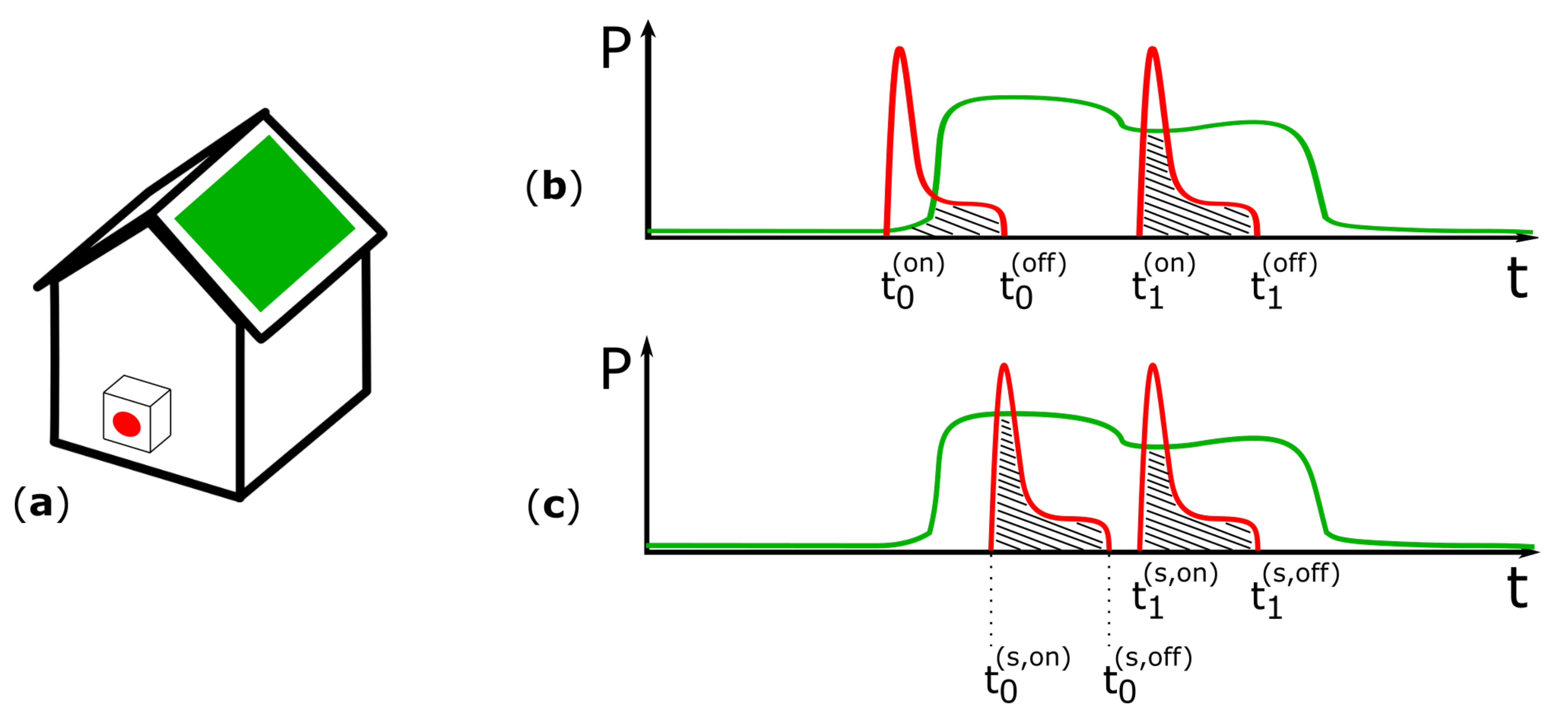
3.4. Increasing Self-Consumption Using Load Shifting
Load shifting algorithms pursue the goal of maximizing
by finding an optimal set of time shifts
to be applied to the appliance activations. Graphically, this concept is represented in
Figure 1. Formally, we can consider the shifts as elements of a matrix
, where
is the maximum number of activations.
The maximization problem is subject to the following constraints: We can shift only in the future (
) and a user might set limits concerning when a certain appliance should have completed an activation. The set of optimal shifts which can be targeted in practice, that is, using sampled signals, is then:
The estimated optimal self-consumed energy after load shifting is then expressed as follows:
It is worth pointing out that optimizing the choice of the time shifts in real time as a user decides to switch on an appliance presents further challenges which are out of the scope of the present work: The signal can only be predicted through weather models and is therefore not necessarily accurate. In our simulations we aim at evaluating the potential improvements in retrospective, assuming that we know the whole signals already.
3.5. Activation Detection
In order to perform load shifting, we need to first estimate the activation times from the available power signals for each appliance. This means that we need to estimate and from the power trace of each appliance.
To this end we proceed with the following heuristic approach. For each house and appliance, we choose manually parameters describing the typical range of energy usage and duration for an activation, as well as a minimum power draw at some point during the activation. We first determine which samples in the power signal are above the minimum power threshold and these are grouped. Samples over the threshold are grouped whenever the grouping creates a block which has a duration close to the typical activation duration for a certain appliance. Samples falling between those which belong to the same group are assigned to that same group even if they are below the power threshold. Candidate groups are assessed for the whole set of possible appliances.
The raw grouping algorithm is intentionally biased towards incorrectly combining nearby appliance activations, rather than separating a single activation into multiple groups. We augment the grouping algorithm with a splitting pass. For each identified group, we consider splitting it into n groups, each with an equal number of samples. The algorithm optimizes a cost function to determine the best n. For each of the n candidate groups, the total energy used by the appliance within the candidate activation is calculated. The cost function is created by measuring the difference between the total candidate energies, so that the algorithm chooses splits where every new group has a total energy close to the typical energy for that appliance, and where all new groups have approximately equal energy consumption.
3.6. Load Shifting Algorithms
Different approaches can be used to maximize the quantity in Equation (
5). The maximization is not trivial, since the form is non-differentiable in the time shifts due to the minimum operator. We use two heuristic methods which differ in the amount of knowledge that is assumed to be known about the household load and production profiles. We call “optimal” the method which has full access to the data and “naive” the one which does not. While for our retrospective analyses we do have access to the full data, the comparison has still practical relevance, since if a system had to be deployed in a real setting, only the “naive” version could be applied.
The two algorithms here presented share the following trivial properties: They can shift activations only to future time points and they can shift each activation so that an appliance gets switched off at latest at the next (original) activation of the same appliance. As an example, if the user runs a washing machine multiple times in quick succession, then only the last activation can be shifted significantly. For both shifting algorithms, the shifts are performed as follows: For each house and appliance, the original (not shifted) power consumption data is loaded. For every activation of the appliance, the algorithm decides the number of samples to shift it by. During the period of the original activation, the appliance power usage is subtracted from the house’s aggregate power usage and the appliance power usage is set to zero. The power usage profile of the original activation is delayed by the chosen time and added back to the modified aggregate and appliance power usage data. It is important to note that we only shift one appliance at a time. For the remaining appliances in a household, the original non-shifted data is used.
3.6.1. Naive Load Shifting
Before applying the naive load shifting algorithm, we identify a time of the day after which the sun irradiance is typically high at the specific location. This should allow us to maximize self-consumption. The specific time will depend on the location and period of the year; in the following let us assume this time to be noon. The naive load shifting algorithm chooses the time shifts as follows: If an appliance was originally started before noon, it is shifted so that it starts exactly at noon. If the appliance was originally started after noon, it is not shifted at all. This algorithm will thus never shift an appliance activation to a different day.
3.6.2. Optimal Load Shifting
This algorithm uses measured aggregate electrical load and PV production data to decide how far to shift each appliance activation. While respecting the common constraints defined above, the algorithm selects a shift distance which maximizes the household’s PV self-consumption. This is done by evaluating Equation (
5) with one appliance at a time and with multiple candidate time shifts. We further constrain the shifted start time to be at most 24 h after the original start time. This algorithm may shift activations to the next day, in contrast to the naive version.
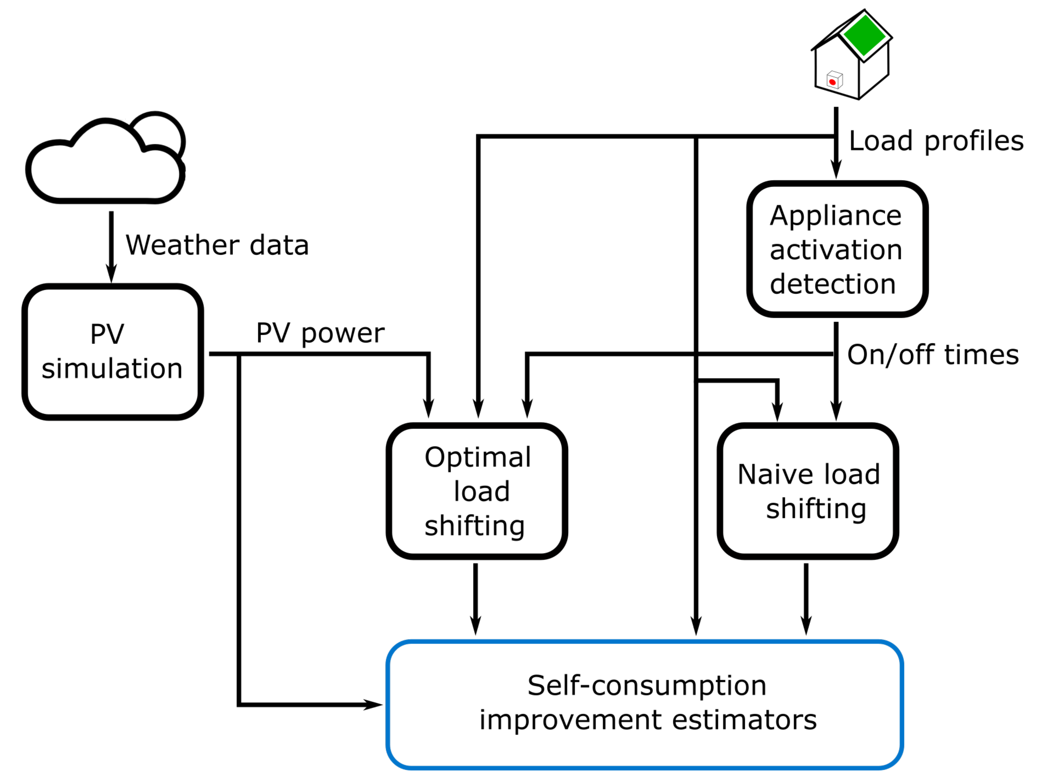
3.7. Simulation Workflow
The focus of this work is to evaluate how the estimated improvement of the self-consumed energy is impacted by the sampling rate used throughout the whole process. Formally, we want to establish a relationship between
T and the estimated improvement
. We argue that
is a biased estimator of the real achievable improvement
and that the amount of bias depends on the sampling rate
T. To prove this we perform experiments where we apply the whole methodology at different sampling rates and we calculate the corresponding set of estimators. The simulation workflow is depicted in a simplified version in
Figure 2.
4. Datasets and Pre-Processing
In this part we illustrate the datasets to which we apply the methodology presented in
Section 3. In order to perform our simulations, we need synchronous data of electrical load and potential PV production for a set of houses. Since we do not have access to such a dataset, we generate the PV data from available weather data.
4.1. Electrical Load Data
Measurements of electrical load were taken from the “REFIT: Electrical Load Measurements (Cleaned)” [
18] dataset. The data were collected between 2013 and 2015. This version of the dataset had forward filling and other cleaning steps performed by the REFIT authors. REFIT contains 20 households, all of which are located in the area of Loughborough, UK (52.7705
N 1.2046
W).
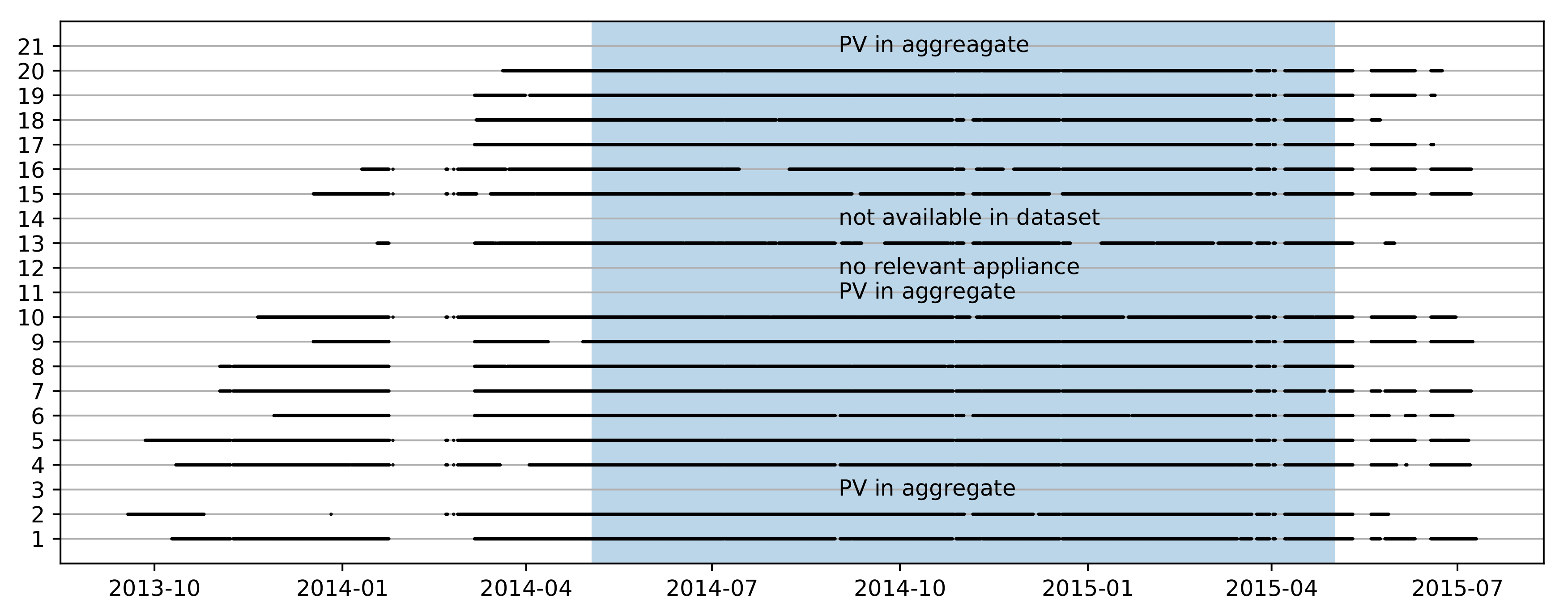
Since our simulations require load measurements from individual appliances, we only used measurements from households for which at least dishwasher, washing machine or tumble dryer measurements were available. This excludes one household (house 12) in which none of these appliances were measured. House 4 had two washing machines, but we only performed load shifting with one (appliance 4). Additionally, we excluded three households (3, 13, 21) where solar power production distorts the recorded aggregate power consumption, as stated in the dataset documentation. Considering these exclusions, we worked with a total of 16 houses which contained a total of 12 dishwashers, 16 washing machines and 9 tumble dryers.
The 16 houses used in our evaluation were constructed in a range of years between 1919 and early 2000s, quite evenly distributed. The number of occupants ranges from 1 to 6, with a median of 2.5. Most of the houses are detached and with sizes ranging from 2 to 5 bedrooms, with a median of 3. According to the 2011 UK census data, most households in the UK have 2 occupants and 3 bedrooms [
19]. The houses used in this study therefore seem to be somehow representative, though the detached houses are here overly represented.
In addition to measurements of the single appliances, we used the aggregate load measurements for each household. For the study, we used the data between the 3rd of May 2014 and the 3rd of May 2015 as indicated with the blue background in
Figure 3. All other data from REFIT were not used. The data in REFIT were recorded with a sampling period of 8 s. The synchronization of appliance and aggregate measurements is discussed in Reference [
18].
4.2. Irradiance Data
The photovoltaic production data which we need to calculate PV self-consumption are simulated based on irradiance measurements. For testing the effect of the sampling rate on self-consumption we required irradiance data with a high sampling rate. This kind of data is difficult to obtain for an arbitrary location and time frame. We chose to use data from the Baseline Surface Radiation Network. The network consists of about 60 stations around the world. The data are measured at 1 Hz and then averaged to a 1 min sampling period before publication [
20].
We used data from the Baseline Surface Radiation Network (BSRN) station in Camborne, UK (50.2167
N 5.3167
W) for the years 2014 and 2015 [
21]. This is the nearest BSRN station to Loughborough, where the electrical load data were collected. The distance between these two sites is 400 km, so the weather conditions at both can differ. We expect that using irradiance data measured in Loughborough would change the self-consumption that we calculate. However, we believe that our combination of data from two locations still represents realistic household consumption and production, since households in both locations likely have similar electricity consumption patterns. Furthermore, our focus here is on the effect of the sampling rate and not on the absolute quantification of the potential improvement in self-consumption for the concrete houses within the REFIT dataset.
In addition to the BSRN irradiance data, our PV simulation used wind speed and air temperature data. These data were collected by the UK Met Office [
22]. These are hourly measurements collected in the same location as the BSRN Camborne station.
4.3. PV Simulation
In order to obtain PV power data, we perform a photovoltaic system simulation using the irradiance and weather data discussed above to estimate the produced AC power. The PV simulations are implemented by pvlib-python [
23]. Wind speed and air temperature data are linearly interpolated to 1 min sampling period to match irradiance data before being fed into pvlib-python. We used the AC power production estimated by pvlib-python as the PV production data for all households in our experiments. The power distribution across phases was disregarded.
The simulated PV system had 12 LG LG290N1C-G3 panels (parameters from the Sandia module database [
24]) for a total of 3480 kWp. The system had a Fronius Primo 3.8-1 208-240 inverter (parameters from the California Energy Commission (CEC) inverter database [
24]). For all other parameters the default values set by pvlib-python were used (see
Appendix A). The total losses in the system made the energy output approximately 17% lower than a value based only on global horizontal irradiance measurements and the power rating of the panels at standard test conditions (STC).
4.4. Combination and Resampling
The electrical load data from REFIT and the AC power production from the PV simulation are used as inputs for load shifting. We first synchronize the datasets, keeping only time intervals where samples from both datasets are available. We then resample both datasets to the desired sampling rates. Sampling rates from 1 min to 10 min in one minute steps have been used. The output of this process generates electrical load data for each house, but identical PV production data for all houses.
4.5. Availability of Data and Materials
The following resources are provided to enable reproducibility:
5. Results
In this section we present our results in terms of estimation of the achievable improvement in the self-consumption and its relation to the sampling rate. In order to show results which are comparable and easy to interpret, we normalize all the energies by the lengths of the datasets, thereby obtaining powers which we report in Wh/day. In order to put the improvements in context, as a first step we calculate a theoretical upper bound for the improvement which would be achievable for each house and appliance in the REFIT dataset. This is done by assuming that each appliance could be powered entirely by the PV production. We denote the estimated maximum improvement with .
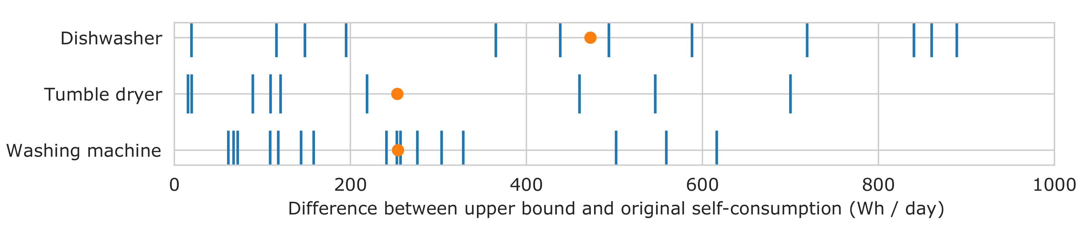
5.1. Theoretical Upper Bound for Improvements
Figure 4 shows the value of the theoretical self-consumption upper bound
broken down by appliance and household. The values are absolute increases in self-consumption compared to the situation before load shifting. There are very large differences between households. The differences between appliances are less pronounced, though the upper bound values for dishwashers are generally higher.
The influence of the sampling rate on the theoretical upper bound for the self-consumption improvement is shown in
Table 1. The second and third columns in
Table 1 report respectively the mean and median of the aggregated upper bound for all houses and appliances, expressed in Wh/day. The upper bound is decreases when increasing the sampling rate. The value at 1 min sampling period (325 Wh/day) is 6% higher than at 10 min sampling period (307 Wh/day). This difference should be considered when viewing results which are relative to the upper bound.
5.2. Results at Fastest Sampling Rate
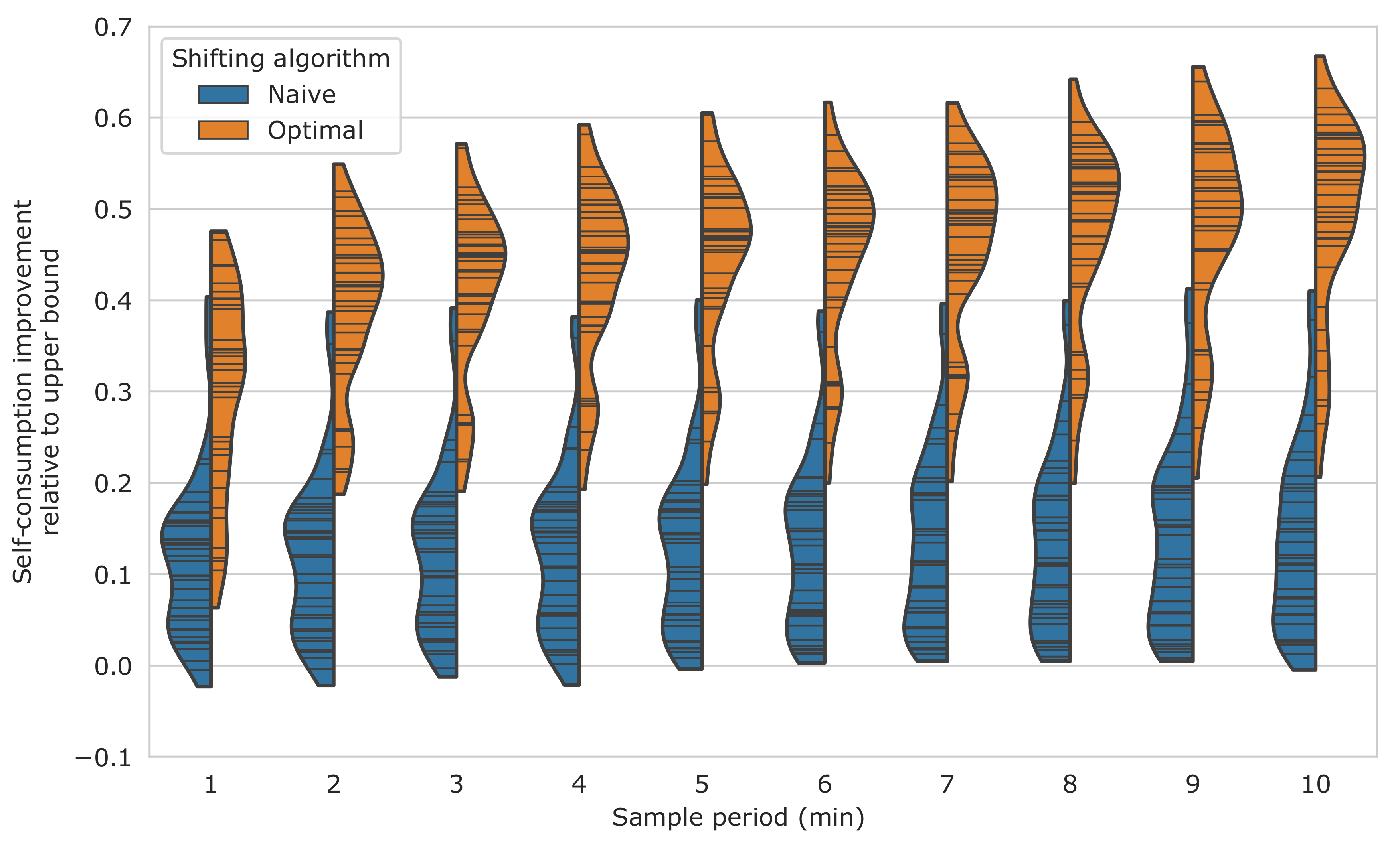
Figure 5 shows one distribution of the self-consumption improvements for each of the considered sampling rates. Each distribution should be read as follows: The blue area on the left half shows the distribution of results from the naive load shifting algorithm. The orange area shows results for the optimal load shifting algorithm. The values are normalized with the upper bound improvement. This means that a value of 1 is the theoretical maximum improvement, which will never be achieved in reality. Each black horizontal line represents a single result and the colored area represent approximations of the distributions of the single results using kernel density estimation.
Consider the first section of
Figure 5, which corresponds to a sampling rate of 1 min. This is the fastest sampling rate which we can work with using our data. We expect these results to be more realistic than the ones calculated with slower sampling rates. Although these results are relative to our upper bound, there are still significant variations between different machines and households. The optimal load shifting algorithm is clearly more effective at increasing PV self-consumption than the naive counterpart. This is also visible in the absolute results from
Table 1 (naive mean: 36.6 Wh/day, optimal mean: 103 Wh/day). In a few cases, the naive algorithm decreased the self-consumption compared to not performing any shifting.
5.3. Influence of Sampling Rate
Consider the entire
Figure 5, with sections for various sampling rates. There is a clear trend in the improvement calculated by the optimal algorithm. For slower sampling rates, the predicted improvement from load shifting is larger. There is an especially pronounced difference between the results with 1 min and 2 min sampling periods. The results from this plot and
Table 1 show that the 1 min simulation predicts 30–40% less self-consumption improvement than the 10 min simulation.
The performance of the naive algorithm shows significantly less influence from sampling rate. The 1 min simulation predicts 15–20% less improvement than the 10 min simulation. This trend is not very noticeable when looking at the curves from the kernel density estimation. The sharp drop from 2 min to 1 min sampling rate for the optimal algorithm does not occur for the naive algorithm.
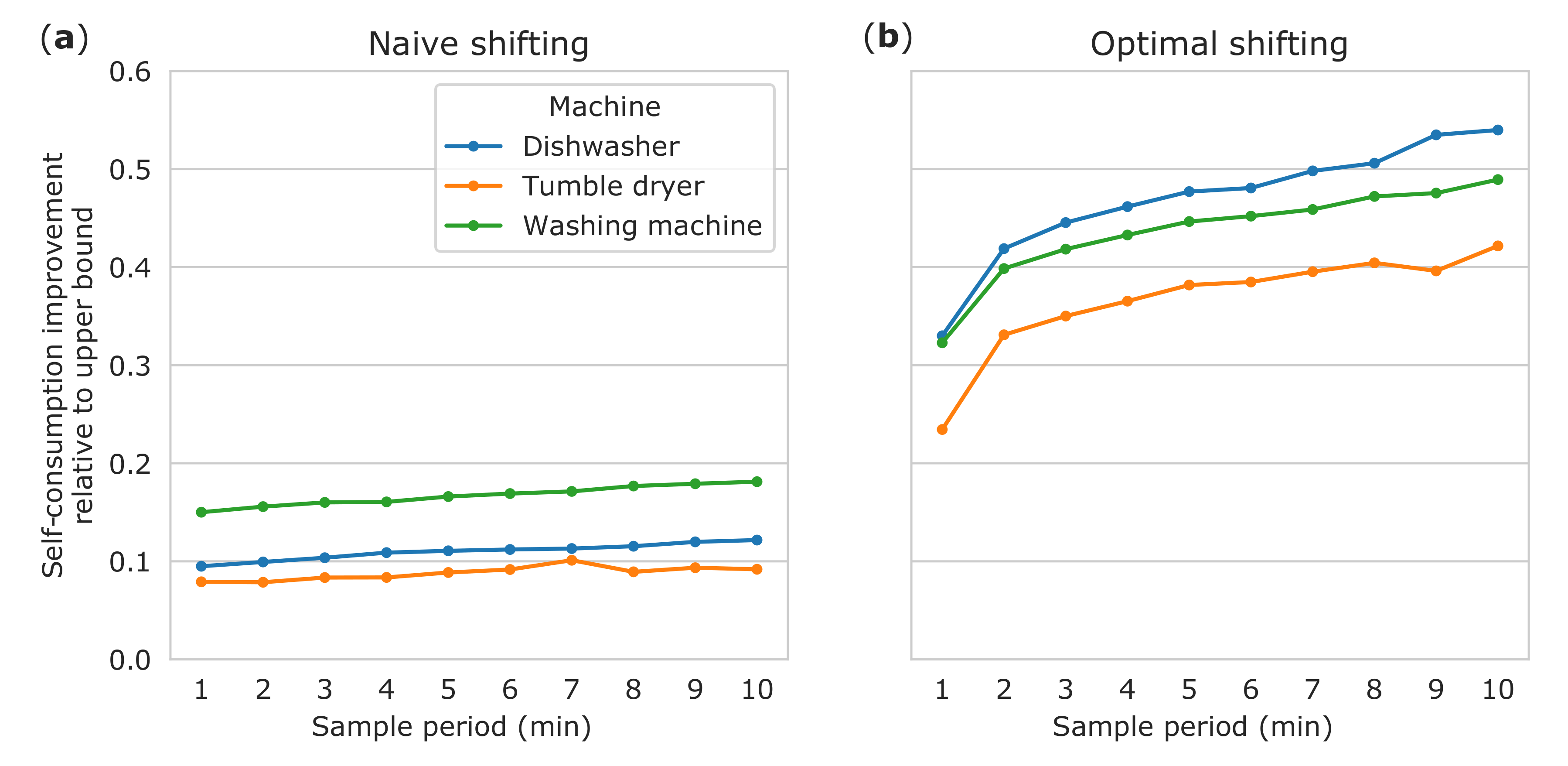
Figure 6 shows the mean self-consumption improvement by machine type. All machines and both algorithms follow the same trend for improvement with varying sampling rate. The dishwasher results change significantly between algorithms, compared with the results for other machines. This is likely because of the different distribution of dishwasher use throughout the day, compared to other appliances. Dishwashers are often run in the evening or at night, while washing machines and tumble dryers are typically used during the day [
5]. Since our naive algorithm is constrained to not shift activations to the next day, it cannot shift evening dishwasher activations to the next morning. The optimal algorithm does not have this limitation.
6. Discussion
6.1. Comparison With Prior Research
In agreement with prior research [
4,
5], we find that the absolute possible improvements in self-consumption due to shifting of appliances are small—on average 37 kWh per year and appliance at 1 min sampling period for the optimal shifting scenario. Assuming a household with a single instance of each investigated appliance, this number adds up to an estimated potential of 110 kWh per year per household. This value is in the same order of magnitude as the 200 kWh [
4] and 129 kWh [
5] found in previous studies. Interestingly, the value seems to be similar even though the data originate from distinct geographic locations: Sweden for Reference [
4], Netherlands for Reference [
5], and the UK in this study. We hypothesize that the load shifting potential of the investigated appliances is similar in European countries.
6.2. Strength of Influence of Sampling Rate
The relative error in the mean upper bound between 1 min and 5 min sampling period is 3%. A similar relative error in self-consumption of around 1% to 6% (depending on the specific house) is also reported in the study of Beck [
6].
With respect to the self-consumption improvement due to appliances, we observe a clear tendency to overestimate the benefit in case of lower sampling rates: Simulations at 1 min predict 30–40% less self-consumption improvement than the 10 min simulation in case of the optimal shifting approach and 15–20% less improvement in case of the naive algorithm. This observation implies that data need a sampling period of at most 1 min (or if possible shorter) to correctly estimate the load shifting potential. The result quantifies the impact of the peak-averaging mechanism introduced in
Section 1. This confirms that the averaging effect on large fluctuations in the load profile introduced at slower sampling rates indeed translates in higher probability that the PV generation peak can be erroneously thought to satisfy the flattened consumption peaks, even when this is not the case.
The observation that data with a 10 min sampling period can introduce significant errors in simulations has consequences for smart meter installations. From an evaluation of smart meter rollouts in EU member states, it was found that around half of the countries use smart meter systems that provide data at sampling periods of 15 min or slower [
25]. This makes the collected data unusable for certain simulations, such as the kind which we have investigated.
6.3. Variation in Prior Research Considering Influence of Sampling Rate
Considering the marked influence of sampling rate on the estimated self-consumption, we suspect that the difference in the reported self-consumption potential between the previous studies can be mainly attributed to the different sampling rates used—Widén [
4] used data with 10 min sampling period and reported 200 kWh potential while Staats [
5] worked on data with 10 s sampling period and reported a smaller potential of 129 kWh.
6.4. Further Considerations
The sample size considered in this study might appear limited, if the number of households is counted. Nevertheless, different households contain very similar appliances and for each household these appliances are used a very high number of times, thus generating hundreds of peaks, each of which might contribute to the wrong self-consumption estimation. Therefore, the actual sample size for the problem at hand is much higher than just the number of households and we believe that our observations are applicable beyond the dataset used in this study.
Using higher sampling rates yields more accurate results at the expense of generating more data. Typically, the data collected by the metering and sub-metering infrastructure can be processed at the edge of the system in order to suggest load-shifting actions to the user or to enact those automatically. If we use a sampling rate of 1 Hz, for example, we need to store 86’400 floating point numbers per day, that is, approximately 320 kB. In a typical practical scenario, short-term load forecasting would be used in combination with a forecast of the PV output in order to infer when a shift in some load would be beneficial to increase self-consumption. Load forecasting was shown to be feasible feeding the last couple of days into a model [
26]. Older data points could then be discarded. This would mean that the edge devices need to store in the order of 1 MB in order to process the information with higher sampling rate. This is feasible with the current infrastructure.
Our simulations are limited to the scenario containing single households and PV data. We could envision extending the present investigation to the level of micro-grids, where load-shifting approaches could be applied to distributed loads in presence of an increased number of stochastic sources of energy, for example, more PVs in conjunction with a small wind turbine and distributed storage systems.
7. Conclusions
Based on measured consumption data from 16 households in the UK and corresponding simulated PV data, we investigated the effect of the sampling rate on the estimated self-consumption potential of shiftable household appliances (washing machines, tumble dryers and dishwashers). Varying the sampling period of our simulation between 1 and 10 min, we found that the results have a marked dependence on sampling rate. Self-consumption evaluated with data with a 10 min sampling period was overestimated by 30–40% compared to data with a 1 min sampling period when using an optimal algorithm for load shifting. When using a naive load-shifting variant, the overestimation was reduced to 15–20%, which is still a relevant amount. We therefore strongly encourage other researches in the field to carefully choose the data rate when delivering estimates of the self-consumption improvement potential with PV and shiftable loads. Furthermore, the results obtained here have a direct practical applicability in the design of edge systems implementing load-shifting mechanisms in households. Finally, in accordance with previous studies, we found that the types of appliances considered have low potential to improve self-consumption.
As a follow-up of the present studies, the simulations could be extended to more households and more diverse settings. A radically different approach would be to perform stochastic simulations of the kind presented in Reference [
10]. The data obtained in this way could be used as a base to investigate the effect of different load-shifting approaches on an arbitrarily diverse dataset. Algorithms taking into account load-shifting, combined with the possibility to store energy could be investigated, including their dependence on the sampling rate used. A further investigation point could be to study which characteristic of the households might have an impact of the potential level of self-consumption.
Author Contributions
Conceptualization, P.V., P.H. and A.R.; methodology, P.V.; software, P.V.; validation, P.H., A.R. and A.P.; formal analysis, P.H. and A.C.; investigation, P.V.; resources, A.P.; data curation, P.V.; writing—original draft preparation, P.V.; writing—review and editing, P.H. and A.C.; visualization, P.V. and A.C.; supervision, A.R. and A.P.; project administration, P.H.; funding acquisition, A.R. and A.P. All authors have read and agreed to the published version of the manuscript.
Funding
This research project is financially supported by the Swiss Innovation Agency Innosuisse (contract number 1155000149) and is part of the Swiss Competence Center for Energy Research SCCER FEEB&D.
Acknowledgments
The authors want to express their gratitude to Thomas Bosser, who contributed to intermediate steps on the way to the final publication.
Conflicts of Interest
The authors declare no conflict of interest. The funders had no role in the design of the study; in the collection, analyses, or interpretation of data; in the writing of the manuscript, or in the decision to publish the results.
Appendix A
The following parameters were used for our PV simulation. Except for the orientation strategy, these are defaults chosen by pvlib-python.
ModelChain:
name: None
orientation_strategy: south_at_latitude_tilt
clearsky_model: ineichen
transposition_model: haydavies
solar_position_method: nrel_numpy
airmass_model: kastenyoung1989
dc_model: sapm
ac_model: snlinverter
aoi_model: sapm_aoi_loss
spectral_model: sapm_spectral_loss
temperature_model: sapm_temp
losses_model: no_extra_losses
References
- Masson, G. Snapshot of Global PV Markets 2020; Snapshot IEA-PVPS T1-37: 2020; International Energy Agency IEA: Paris, France, 2020.
- Luthander, R.; Widén, J.; Nilsson, D.; Palm, J. Photovoltaic self-consumption in buildings: A review. Appl. Energy 2015, 142, 80–94. [Google Scholar] [CrossRef]
- Siano, P. Demand response and smart grids—A survey. Renew. Sustain. Energy Rev. 2014, 30, 461–478. [Google Scholar] [CrossRef]
- Widén, J. Improved photovoltaic self-consumption with appliance scheduling in 200 single-family buildings. Appl. Energy 2014, 126, 199–212. [Google Scholar] [CrossRef]
- Staats, M.; de Boer-Meulman, P.; van Sark, W. Experimental determination of demand side management potential of wet appliances in the Netherlands. Sustain. Energy Grids Netw. 2017, 9, 80–94. [Google Scholar] [CrossRef]
- Beck, T.; Kondziella, H.; Huard, G.; Bruckner, T. Assessing the influence of the temporal resolution of electrical load and PV generation profiles on self-consumption and sizing of PV-battery systems. Appl. Energy 2016, 173, 331–342. [Google Scholar] [CrossRef]
- Braun, M.; Büdenbender, K.; Landau, M.; Sauer, D.U.; Magnor, D.; Schmiegel, A.U. Charakterisierung von netzgekoppelten PV-Batterie-Systemen. In Proceedings of the 2010 25th Symposium Photovoltaische Solarenergie, Bad Staffelstein, Germany, 3–5 March 2010. [Google Scholar]
- Wyrsch, N.; Riesen, Y.; Ballif, C. Effect of the Fluctuations of PV Production and Electricity Demand on the PV Electricity Self-Consumption. In Proceedings of the 28th European Photovoltaic Solar Energy Conference and Exhibition, Paris, France, 30 September–4 October 2013; pp. 4322–4324, IMT-NE Number:733. [Google Scholar] [CrossRef]
- McKenna, E.; Pless, J.; Darby, S.J. Solar photovoltaic self-consumption in the UK residential sector: New estimates from a smart grid demonstration project. Energy Policy 2018, 118, 482–491. [Google Scholar] [CrossRef]
- Leicester, P.A. Probabilistic analysis of solar photovoltaic self-consumption using Bayesian network models. IET Renew. Power Gener. 2016, 10, 448–455. [Google Scholar] [CrossRef]
- Swain, K.P.; De, M. Analysis of Effectiveness of Flexible Load Shifting Order on Optimum DSM. In Proceedings of the 2017 IEEE International WIE Conference on Electrical and Computer Engineering (WIECON-ECE), Uttarkhand, India, 18–19 December 2017; pp. 141–144. [Google Scholar]
- Ran, X.; Leng, S. Enhanced Robust Index Model for Load Scheduling of a Home Energy Local Network with a Load Shifting Strategy. IEEE Access 2019, 7, 19943–19953. [Google Scholar] [CrossRef]
- Liao, Z.; Gu, X. Research on the peak load shifting plan optimization based on TABU search algorithm. In Proceedings of the 2014 IEEE PES Asia-Pacific Power and Energy Engineering Conference (APPEEC), Kowloon, Hong Kong, 7–10 December 2014; pp. 1–5. [Google Scholar]
- Balakumar, P.; Sathiya, S. Demand side management in smart grid using load shifting technique. In Proceedings of the 2017 IEEE International Conference on Electrical, Instrumentation and Communication Engineering (ICEICE), Karur, India, 27–28 April 2017; pp. 1–6. [Google Scholar]
- Lakshmanan, V.; Marinelli, M.; Kosek, A.M. Thermostat controlled loads flexibility assessment for enabling load shifting—An experimental proof in a low voltage grid. In Proceedings of the 2017 52nd International Universities Power Engineering Conference (UPEC), Crete, Greece, 28–31 August 2017; pp. 1–6. [Google Scholar]
- Yasin, A.; Khan, S.A. Unsupervised Event Detection and On-Off Pairing Approach Applied to NILM. In Proceedings of the 2018 International Conference on Frontiers of Information Technology (FIT), Islamabad, Pakistan, 19–21 December 2018; pp. 123–128. [Google Scholar]
- You, Z.; Raich, R.; Huang, Y. An inference framework for detection of home appliance activation from voltage measurements. In Proceedings of the 2014 IEEE International Conference on Acoustics, Speech and Signal Processing (ICASSP), Florence, Italy, 4–9 May 2014; pp. 6033–6037. [Google Scholar]
- Murray, D.; Stankovic, L.; Stankovic, V. An electrical load measurements dataset of United Kingdom households from a two-year longitudinal study. Sci. Data 2017, 4, 160122. [Google Scholar] [CrossRef]
- UK Census. 2011. Available online: http://www.nomisweb.co.uk/census/2011 (accessed on 1 October 2020).
- Driemel, A.; Augustine, J.; Behrens, K.; Colle, S.; Cox, C.; Cuevas-Agulló, E.; Denn, F.M.; Duprat, T.; Fukuda, M.; Grobe, H.; et al. Baseline Surface Radiation Network (BSRN): Structure and data description (1992–2017). Earth Syst. Sci. Data 2018, 10, 1491–1501. [Google Scholar] [CrossRef]
- Tamlyn, J. Basic Measurements of Radiation at Station Camborne (2014-01 to 2015-12, 24 Datasets); Met Office: Exeter, UK; PANGAEA: Exeter, UK, 2016. [Google Scholar]
- Met Office. MIDAS Open: UK Hourly Weather Observation Data, v201908; Centre for Environmental Data Analysis: Chilton, UK, 2019. [Google Scholar] [CrossRef]
- Holmgren, W.F.; Hansen, C.W.; Mikofski, M. pvlib python: A python package for modeling solar energy systems. J. Open Source Softw. 2018, 3, 884. [Google Scholar] [CrossRef]
- System Advisor Model Version 2020.2.29; SAM Source Code; National Renewable Energy Laboratory: Golden, CO, USA, 2020. Available online: https://github.com/NREL/ssc (accessed on 1 June 2020).
- Tounquet, F.; Alaton, C. Benchmarking Smart Metering Deployment in the EU-28; Publication Office of the EU: Luxembourg, 2020. [Google Scholar] [CrossRef]
- Pellegrini, M. Short-term load demand forecasting in Smart Grids using support vector regression. In Proceedings of the 2015 IEEE 1st International Forum on Research and Technologies for Society and Industry Leveraging a Better Tomorrow (RTSI), Torino, Italy, 16–18 September 2015; pp. 264–268. [Google Scholar]
| Publisher’s Note: MDPI stays neutral with regard to jurisdictional claims in published maps and institutional affiliations. |
© 2020 by the authors. Licensee MDPI, Basel, Switzerland. This article is an open access article distributed under the terms and conditions of the Creative Commons Attribution (CC BY) license (http://creativecommons.org/licenses/by/4.0/).


