Development of Decision-Making Tool and Pareto Set Analysis for Bi-Objective Optimization of an ORC Power Plant

Abstract

Power plants based on organic Rankine cycle (ORC) are known for their capacity in converting low and medium-temperature energy sources to electricity. To find the optimal operating conditions, a designer must evaluate the ORC from different perspectives including thermodynamic performance, technological limits, economic viability, and environmental impact. A popular approach to include different criteria simultaneously is to formulate a bi-objective optimization problem. This type of multi-objective optimization (MOO) allows for finding a set of optimal design points by defining two different objectives. Once the optimization is completed, the decision-making analysis shall be carried out to identify the final design solution. This study aims to develop a decision-making tool for facilitating the choice of the optimal design point. The proposed procedure is coded in MATLAB based on the commonly used Technique for Order Preference by Similarity to Ideal Solution (TOPSIS). By providing the capability to graphically identify the decisions taken, the tool developed in the study is called Tracking and Recognizing Alternative Design Solutions (TRADeS). Analysis of our data shows that certain regions of Pareto set points should be excluded from the design space. It was noted that in these regions a high rate at which one of the objectives moves away from its ideal value coincides with a low rate at which the second criterion approaches its ideal solution. Hence, it was recommended that the criteria weights corresponding to excluded regions of the Pareto set should be discarded when selecting the final design point. By comparing the results obtained using the proposed model to those of existing decision-making techniques, it was concluded that while the known approaches are appropriate for an easy and fast selection of the final design point, the presented procedure allows for a more comprehensive and well-rounded design. It was shown that our design tool can be successfully applied in the decision-making analysis for problems that aim at optimizing the ORC using two design criteria. Finally, the proposed software benefits from a generic structure and is easy to implement which will facilitate its use in other industrial applications.

1. Introduction

The depletion of fossil fuels combined with increasing electricity demand is the main reason for the efforts aiming at the utilization of alternative energy sources. As a technology capable of converting renewable and waste heat to electricity, the organic Rankine cycle (ORC) power plant has been widely investigated in the last decade. The growing interest in developing ORC systems is partly because it lends itself well to applications including geothermal energy [1], solar thermal energy [2], biomass energy [3], and low-grade waste heat recovery [4]. Furthermore, the system can be successfully adapted to a low [5] and medium [6] temperature energy sources due to great variety of possible working fluids, including refrigerants [7], hydrocarbons [8] or siloxanes [9].

The main goal of most ORC-related studies is to evaluate the system performance from different perspectives such as thermodynamic performance, economic viability, or environmental impact. One way to include various aspects simultaneously is to formulate a bi-objective optimization problem. This approach allows for finding a set of optimal solutions (Pareto front) by defining two criteria. The obtained solutions are non-dominated and to choose a better design point with respect to one objective, the second criterion can be compromised. To facilitate the decision-making process, different techniques have been developed throughout the years. Many of these methods have proved to be effective in selecting the final optimal point in ORC power plants.

As stated in the study by Feng et al. [10], Linear Programming Technique for Multidimensional Analysis of Preference (LINMAP) [11] and Technique for Order Preference by Similarity to Ideal Solution (TOPSIS) [12] are among the most commonly applied decision-making methods for supporting the choice of the final design point among Pareto solutions. The LINMAP, also known as an ideal point method [13], is a technique based on the pair-wise comparisons of alternatives (Pareto solutions). The best solution is determined by indicating an alternative that has the shortest distance from a hypothetical ideal point. TOPSIS ranks the Pareto set points similar to LINMAP. Specifically, an alternative point that has the shortest distance from the ideal point and the longest distance from the non-ideal solution is considered as the final design point. It should be noted that both approaches allow for defining the decision-maker preferences by assigning weights to each criterion.

Application of LINMAP and TOPSIS is reported in the papers concerning the optimization of ORCs. Behzadi et al. [14] conducted a bi-objective optimization of the biomass-fired proton exchange membrane fuel cell integrated with ORC and thermoelectric generator. The authors defined the net power output and total cost rate (in $ h⁻¹) as objective functions. To indicate the final design point on Pareto front, the ideal point method was applied. By applying the same approach for the decision-making process, Oyekale et al. [15] found the optimal operating point of the biomass retrofit for an existing ORC power plant. Wu et al. [16] analyzed a novel dual-functional integration system and recorded conflict between the total cost and payback period of the installation. To determine the optimal geothermal water inlet temperature, they conducted a multi-objective optimization and applied the LINMAP as a decision-making procedure. Pourrahmani and Moghimi [17] proposed a new solar-driven integrated system for co-producing of electricity, hydrogen and cooling. The authors applied the genetic algorithm as an optimization tool and the TOPSIS as a decision-making procedure to find the compromised design point. Shen et al. [18] introduced the energy flow model for the modelling and optimization of the ORC systems. Having carried out a bi-objective optimization with the net power output and thermal efficiency as the criteria, the final design points using the TOPSIS approach was determined. Wang et al. [19] conducted a performance comparison of different working fluid pairs for a dual-loop ORC utilizing the waste heat from the engine. By defining the exergy efficiency and payback period as the objective functions, the authors performed a multi-objective optimization using the Non-dominated Sorting Genetic Algorithm (NSGA-II). The Pareto solutions obtained for each working fluid pair were compared using the TOPSIS procedure.

Despite the fact that LINMAP and TOPSIS allow for specifying the decision-maker preferences, there is a need to emphasize assigning weights to the optimization criteria. It should be noted that there are two types of approaches for assigning weights to the objectives. In the first one, the weights are assigned subjectively based on the decision-maker’s knowledge and experience [20]. With the second approach, the criteria weights are determined using objective methods [21]. An exemplary application of the latter procedure was presented in the study by Bina et al. [22]. The authors evaluated the performance of four geothermal-based ORCs by conducting a thermo-economic analysis. To rank different system architectures, the authors defined five optimization criteria and applied the fuzzy TOPSIS as a decision-making tool. The criteria weights were determined using Shannon’s entropy method [23]. Wang et al. [24] conducted a bi-objective optimization of the binary flashing cycle (BFC) considering the net power output and heat exchanger area as two conflicting criteria. By applying NSGA-II, they found the Pareto optimal solutions. To examine various design points, the authors used TOPSIS with a weight factor for the net power output varying in a range from 0.0 to 1.0. The values between 0.1 and 0.6 have been reported as optimal. By limiting the range of the weights, the subjective decision-making process was facilitated. Detchusananard et al. [25] optimized a steam biomass gasification system coupled with the solid oxide fuel cell by solving a bi-objective optimization problem with two economic criteria. To comprehensively evaluate the obtained results, the authors applied ten selection methods, including LINMAP and TOPSIS approaches. Different decision-making results have been compared by varying the weights of the objectives in a range between 0.1 and 0.9. It was reported that for the same weight distributions, LINMAP and TOPSIS provided similar outcomes.

Previous studies on the decision-making process show that it is as essential as the optimization procedure and it should be conducted thoroughly to design the system comprehensively and reliably. Hence, this study aims to develop a decision-making tool to facilitate the choice of the final design point in ORC power plants. The proposed software is based on the well-established TOPSIS procedure. The decisions that can be made during the program operation include covering the desired decision-makers’ preferences, selecting the dominant criterion, or specifying a superiority of the selected objective using a rating scale. New recommendations concerning the decision-making process are presented. In particular, exclusion of weight distributions that correspond to adverse Pareto set points is put forward. These design points are located in regions where a steep rate at which the first objective moves away from its ideal value is combined with a gradual rate at which the second criterion approaches its ideal solution. The consideration of design points that are getting closer to the ideal value of one of the criteria is questionable since a slight improvement of this criterion is accompanied by a significant deterioration of the second objective. The literature review clearly reveals that the discussed effect was not addressed in previous studies. Overall, the main contributions of this study can be listed as (1) Developing an intuitive tool that can be applied in the decision-making process for a bi-objective optimization of the ORC or other industrial systems, (2) Making the developed software code available for public use (3) Making recommendations concerning the criteria weights and the selection of final system design.

2. Analysis and Modeling

2.1. System Description

The system under consideration is modeled as a basic subcritical ORC power plant. As depicted in Figure 1a, the simple ORC consists of a condenser, pump, vapor generator, and turbine coupled with an electric generator. In each of the system devices, the working fluid of organic origin undergoes thermodynamic processes presented in Figure 1b. During the expansion process (1–5) in a turbine, the energy of the working medium is converted into mechanical work of the shaft which is used to drive the electric generator. Then, the working fluid is directed to the condenser in which it is cooled down (5–5”) and condensed (5”–6), by transferring the heat with cold water. In a pump, the medium is pressurized (6–7) to achieve a high-pressure state before entering the vapor generator. Utilizing the heat of geothermal water in the vapor generator, the working fluid is preheated (7–8), evaporated (8–9) and superheated (9–1) to re-enter the turbine and start a new cycle.

2.2. Modeling of ORC Components

The expansion device of the examined system is modeled as a radial-inflow turbine (RIT). RIT converts low enthalpy of the working fluid to shaft work in a compact single-stage structure. Hence, the RIT prevailed as an excellent choice for small-scale ORC systems [27]. As seen in Figure 1b, the expansion of the working fluid is divided into sub-processes that take place within the RIT including volute, nozzle, interspace, and rotor. The modeling of the RIT is based on a mean-line (one-dimensional) model [28] which assumes that the working fluid parameters change only with respect to mean streamline through the individual stage components.

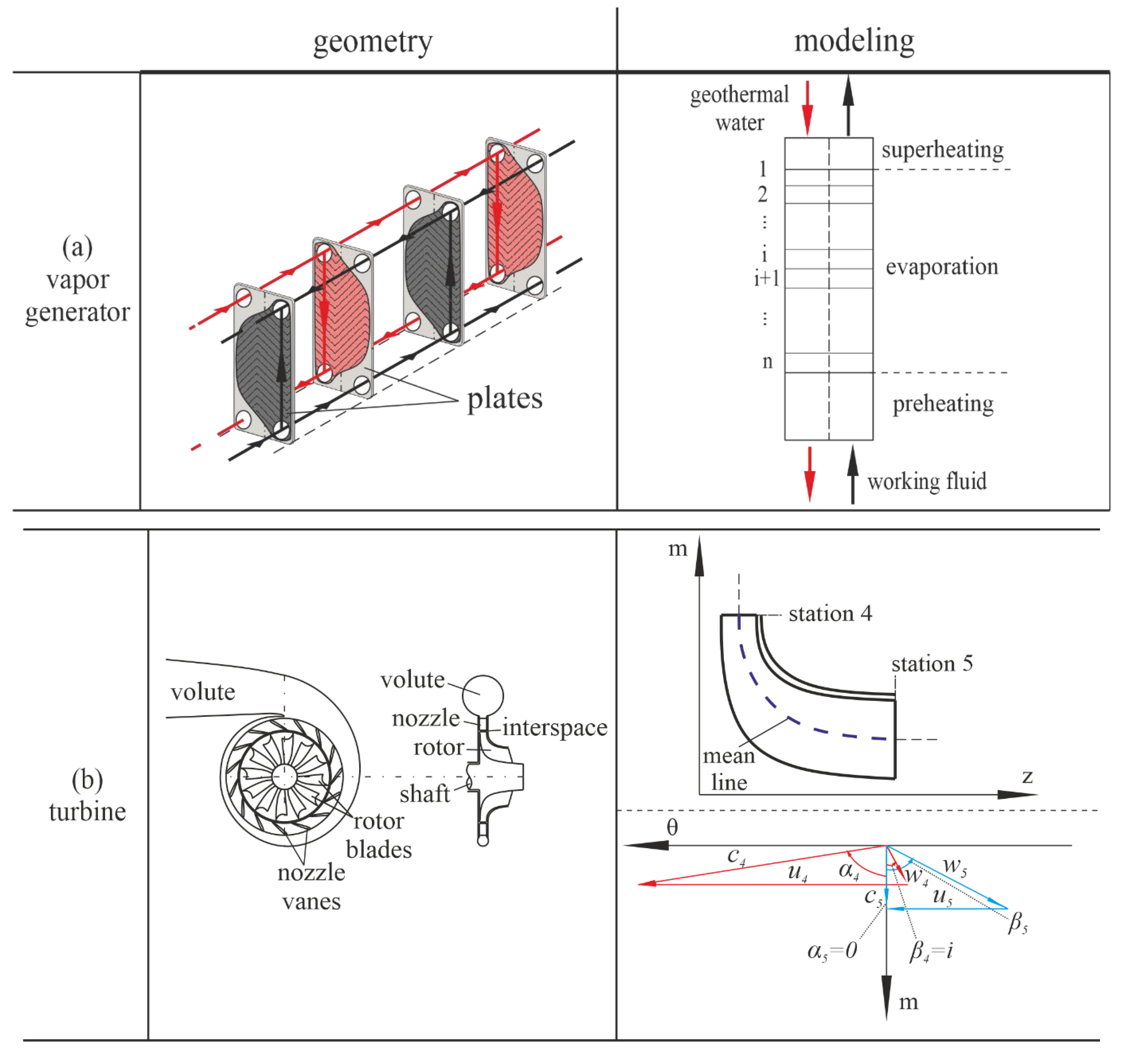
In the preliminary design of the RIT, most attention is focused on the analysis of the flow through the rotor [29]. The cross-section of the rotor with mean streamline drawn between its inlet (4) and outlet (5) stations is depicted in Figure 2b. Furthermore, the velocity triangles at the rotor inlet (parameters with subscript 4) and outlet (parameters with subscript 5) are also presented. The common practice in designing the RIT is to assume the radial blades at the rotor inlet [30] which is equivalent to set the blade angle β_4,blade to 0° (the positive sign of an angle is measured according to the positive direction of peripheral velocity u). For this reason, the relative flow angle and the incidence angle are equal (β₄ = i) since the latter is defined as $i={\beta }_4-{\beta }_{4,blade}$. To ensure no swirl flow at the rotor outlet, the absolute flow angle α₅ is assumed to be equal to 0° [31].

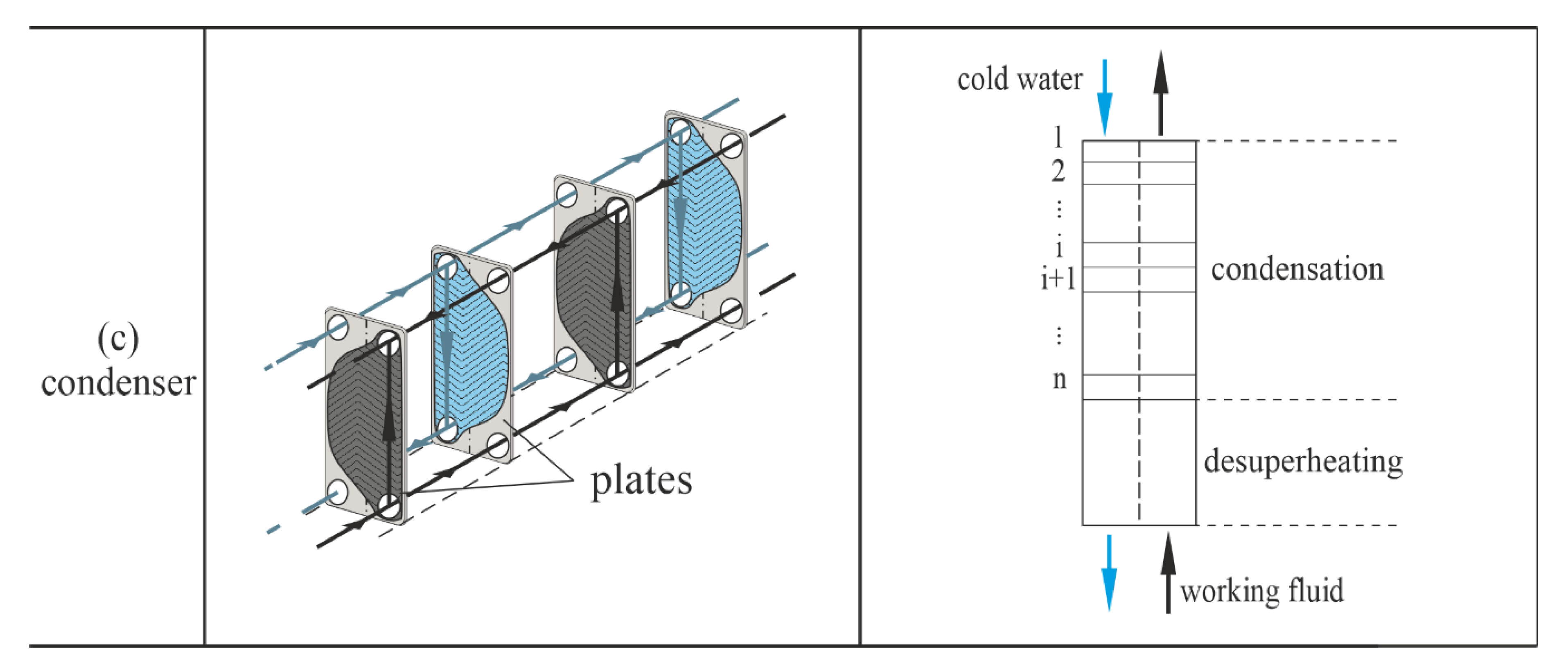
Because of the high heat transfer performance, flexible thermal sizing, and compact dimensions, plate heat exchangers proved to be particularly suitable for ORC power plants [32]. As depicted in Figure 2a,c, this type of heat exchanger geometry is applied to the vapor generator and condenser. Regarding the modeling assumptions, the vapor generator is divided with respect to the thermodynamic processes of the working fluid, including preheating, evaporation, and superheating. Evaporation is a two-phase process that is characterized by the rapid changes in the thermophysical properties of the fluid. For this reason, the evaporation is discretized into n sub-processes and the value of n = 10,000 is assumed as it provides high accuracy of the calculation procedure. Similarly, the condenser is divided into sections in which de-superheating and condensation processes take place. As the condensation is also a two-phase process, it is modeled in the same manner as the evaporation of the working fluid.

As a common practice in designing the ORC, the pump of a system is modeled as a device working with a constant efficiency [33].

2.3. Assumptions and Calculation Steps

The calculation model is built in a form of the originally developed code written in MATLAB environment [34]. The detailed description of the modeling is out of the scope of this study. Nevertheless, the individual calculation steps are briefly explained using a simplified flowchart presented in Figure 3.

The procedure starts by assigning values to the input variables including the volumetric flow rate of the geothermal water ${\dot{V}}_{gw}$, the inlet temperature of the geothermal water T_gw1, the inlet temperature of the cold water T_cw1, and thermophysical properties of the working fluid applied in the ORC. At this stage of the modeling, the decision variables are specified as well and they include the evaporation temperature T_eva, the condensation temperature T_con, the specific speed n_s, and the temperature difference at the saturation liquid point ΔT_eva (see Figure 1b). The first, the second, and the last parameter strongly affect the thermodynamic performance of the ORC. The third variable is closely related to the turbine efficiency and it is defined as follows:

$$n_s=\frac{\omega {\left(\frac{{\dot{m}}_{wf}}{{\rho }_{05}}\right)}^{0.5}}{{\left(h_{01}-h_{5s}\right)}^{0.75}}$$

(1)

The detailed description of the decision variables and their limits can be found in [26]. Furthermore, the assumed operating parameters of the ORC are the same as those in [26] as listed in

Table 1. Operating parameters of the ORC [26].

Parameter	Unit	Value	Type of Variable
${\dot{V}}_{gw}$	[m3 h−1]	30.0	constant value
Tgw1	[°C]	120	constant value
sal	[kgkg−1]	0.00	constant value
fluid	[-]	R1234yf	constant value
ΔTsup	[K]	5.00	constant value
ΔTeva	[K]	see Equation (15)	decision variable
ΔTcon	[K]	5.00	constant value
Tcw1	[°C]	15.0	constant value
ηT	[%]	75.0	design variable
ns	[-]	see Equation (14)	decision variable
ηP	[%]	75.0	constant value
Teva	[°C]	see Equation (12)	decision variable
Tcon	[°C]	see Equation (13)	decision variable

.

To calculate basic thermodynamic parameters, including the mass flow rates or the temperature distributions of the fluids (geothermal water, working fluid, cold water), each component (or part of the component) of the ORC is considered as a control volume. Assuming that each process in the components (or subcomponents) is a steady-state, the mass, and energy balance equations can be written as follows:

$${\displaystyle \sum }{\dot{m}}_{in}={\displaystyle \sum }{\dot{m}}_{out}$$

(2)

$${\displaystyle \sum }{\dot{m}}_{in}{h}_{in}+\dot{Q}={\displaystyle \sum }{\dot{m}}_{out}{h}_{out}+P_{out}$$

(3)

For determination of the working fluid properties (such as the specific enthalpy h or specific entropy s), REFPROP 9.0 [35] database is employed.

Using the parameters determined in the previous step, the radial-inflow turbine is designed according to the procedure partly discussed in [26]. The key output variable at this stage is a turbine total-to-static efficiency which is calculated iteratively using the following formula:

$${\eta }_T=\left(1-\frac{\Sigma \Delta h_{loss}}{h_{01}-h_{5s}}\right)·100\%$$

(4)

The value of the η_T given in Table 1 serves as an initial guess and it is updated until the convergence of the iterative procedure is ensured. The sum of the enthalpy losses ΣΔh_loss involves exit velocity loss, incidence loss, passage loss, tip clearance loss, trailing edge loss, windage loss, and nozzle loss. The individual losses are calculated based on the empirical models available in the literature. While detailing such models is beyond the scope of this study, loss correlations similar to those in [36] were applied with detailed explanation for the specific enthalpies h₀₁ and h_5s given in [37].

In the next step, the thermodynamic and heat transfer analyses are conducted to determine the ORC performance indicators including the exergy efficiency η_ex and total heat transfer area A_tot. The η_ex is calculated as [38]:

$${\eta }_{ex}=\frac{P_{out}}{{\dot{B}}_{gw1}}·100\%$$

(5)

The A_tot is determined as the sum of the heat transfer areas of the vapor generator and condenser. To calculate the heat transfer areas corresponding to the individual sections of the vapor generator (preheating, evaporation, superheating) and condenser (de-superheating, condensation), the following formula is applied [39]:

$$A=\frac{\dot{Q}}{k\Delta T_{\log }}$$

(6)

The detailed explanation concerning the indicators given in Equations (5) and (6) is presented in [40].

In the next stage, the optimization problem is formulated by defining the objective functions and constraints imposed on the decision variables (see Optimization problem section). Then, the optimal solutions can be found applying the Non-dominated Sorting Genetic Algorithm-II (NSGA-II) [41] which is a tool embedded in MATLAB. When the solutions are determined, they are displayed in a form of the Pareto front graph, a well-known graphical representation of the bi-objective optimization results. Additionally, the numerical values of the outcomes are given as the matrices of the objective functions F and decision variables DV, which completes the procedure.

2.4. Validation of the Calculation Model

The verification of the algorithm which is applied in this work was presented in [37]. By comparing the results generated by the developed procedure with those presented in the literature, it was shown that the presented calculation model leads to reliable findings.

3. Bi-Objective Optimization

It is possible to include different performance aspects simultaneously. Hence, a multi-objective approach has attracted a lot of attention in optimizing the operation of the ORC. As mentioned before, a bi-objective optimization has become especially popular in that field. The mathematical formulation of bi-objective optimization (BOO) can be written as follows:

$$\underset{\overrightarrow{X}}{\min }{f}_1(\overrightarrow{X}),f_2(\overrightarrow{X})$$

(7)

subject to

$$g_i(\overrightarrow{X})\le 0,i=1,\dots ,m$$

(8)

$$h_j(\overrightarrow{X})=0,j=1,\dots ,p$$

(9)

The BOO can be described as minimizing the objective functions f₁ and f₂ (Equation (7)) over a vector $\overrightarrow{X}$, while satisfying the constraints expressed in Equations (8) and (9). The case in which the criterion is to be maximized can be treated by negating the objective function. The vector $\overrightarrow{X}$ of the decision variables are expressed as:

$$\overrightarrow{X}={\left[x_1,x_2,\dots ,x_n\right]}^T$$

(10)

In the literature, there are many methods for dealing with multi-objective optimization (MOO) problems. As one of the most commonly applied optimization techniques [42], Non-dominated Sorting Genetic Algorithm-II (NSGA-II) is used in this study.

Optimization Problem

The optimization problem which was analyzed in [26] is recalled in this paper. Following the notation presented in Equations (7)–(9), the discussed BOO problem can be formulated as follows:

$$\underset{\overrightarrow{X}}{\min }-{\eta }_{ex}(\overrightarrow{X}),A_{tot}(\overrightarrow{X})$$

(11)

subject to

$$60.0{ }^{°}\mathrm{C}\le T_{eva}\le 90.0{ }^{°}\mathrm{C}$$

(12)

$$25.0{ }^{°}\mathrm{C}\le T_{con}\le 40.0{ }^{°}\mathrm{C}$$

(13)

$$0.40\le n_s\le 0.70$$

(14)

$$3.00{ }^{°}\mathrm{C}\le \Delta T_{eva}\le 20.0{ }^{°}\mathrm{C}$$

(15)

$$M{a}_4\le 1.50$$

(16)

$$M{a}_5\le 1.00$$

(17)

$$Z_R\ge 1.50b_4$$

(18)

$$\frac{r_{5,sh}}{r_4}\le 0.78$$

(19)

$$\frac{r_{5,hub}}{r_{5,sh}}\ge 0.40$$

(20)

$$0.45\le R\le 0.65$$

(21)

$$-{40.0}^{°}\le i\le {0.00}^{°}$$

(22)

$$T_{gw2}\ge 60.0{}^{°}\mathrm{C}$$

(23)

The vector $\overrightarrow{X}$ consists of the following decision variables:

$$\overrightarrow{X}={\left[T_{eva},T_{con},n_s,\Delta T_{eva}\right]}^T$$

(24)

In Equation (11) the problem of maximizing the exergy efficiency η_ex while minimizing the total heat transfer area A_tot is formulated. The bounds for the decision variables are presented in Equations (12)–(15). The constraints providing a rational design of the radial-inflow turbine are expressed in Equations (16)–(22). The practical limitation imposed on the outlet temperature T_gw2 of the geothermal water, which allows avoiding the silica oversaturation, is presented in Equation (23). A more detailed description of the optimization problem can be found in [26].

4. Development of Decision-Making Tool

4.1. General Concept and Weighting Technique

The main feature of the proposed tool is the possibility of tracking the decisions taken by graphically indicating the extent to which the selected Pareto set points deviate from the ideal solution. For this reason, the developed software is called TRADeS (Tracking and Recognizing Alternative Design Solutions) which is developed in MATLAB (the program code is available under the link given in Supplementary Materials). The core of the developed procedure is the TOPSIS method which proved to be an effective technique for the decision-making process. The detailed description of the TOPSIS procedure was presented in [26].

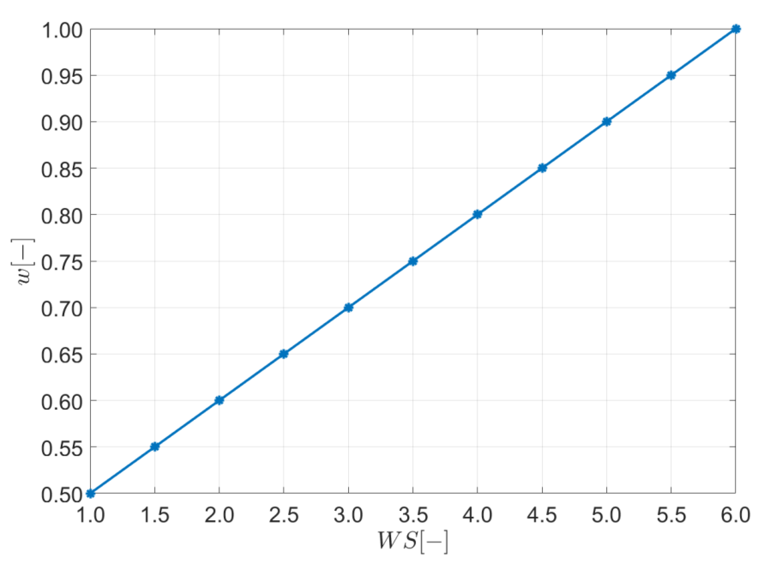
It is worth noting that TOPSIS allows for specifying user preferences by setting weights to the criteria. The problem of assigning weights to the objectives is solved by applying a rating scale between 1.0 and 6.0. For this purpose, the weight superiority WS parameter is introduced. The WS is defined by assuming the linear relationship between the rating that is selected by the user and the weight that is assigned to the objective. Thereby, the weight w is determined using the following formula:

$$w=\frac{WS-up}{2\left(up-low\right)}+1$$

(25)

where low and up are the lower (1.0) and upper (6.0) bounds of the adopted rating scale. The graphical illustration of the results from Equation (25) is presented in Figure 4. As seen, the WS = 1.0 is equivalent to assign w = 0.5, while by assigning WS = 6.0, the weight is equal to w = 1.0. In the case of the BOO, two criteria weights, w₁ and w₂, must be specified. By specifying one of the weights, the second one is always determined using the following relationship:

$$w_2=1.0-w_1$$

(26)

Therefore, assigning the WS to one of the objectives is equivalent to specifying to what extent the selected objective is superior to the other.

4.2. Description of the Procedure

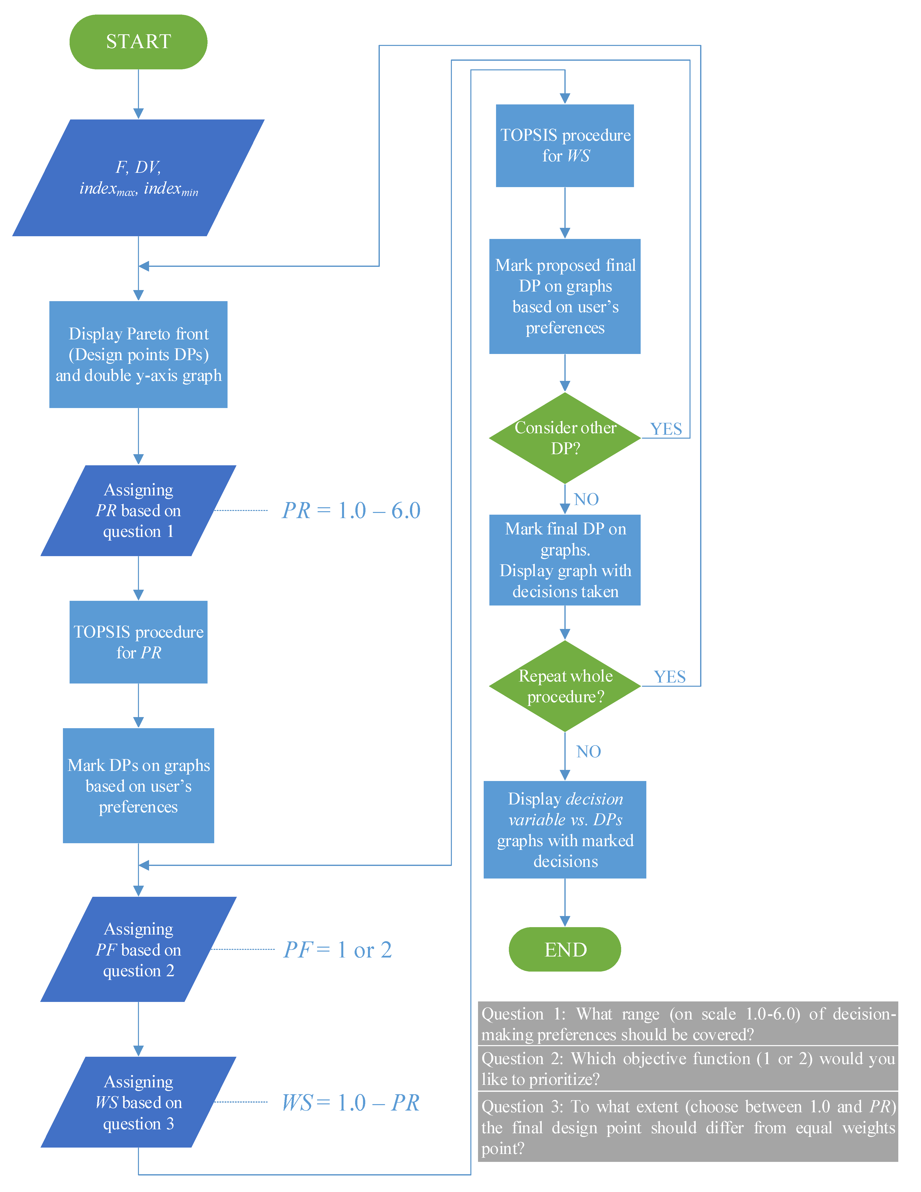
The procedure (see Figure 5) starts from providing the matrices of the objective functions F and decision variables DV which are the outputs of the bi-objective optimization (see Figure 3). The user should also provide the information which objective function is the cost (to be minimized) and benefit (to be maximized) criterion by assigning the column numbers of the F to index_min and index_max parameters.

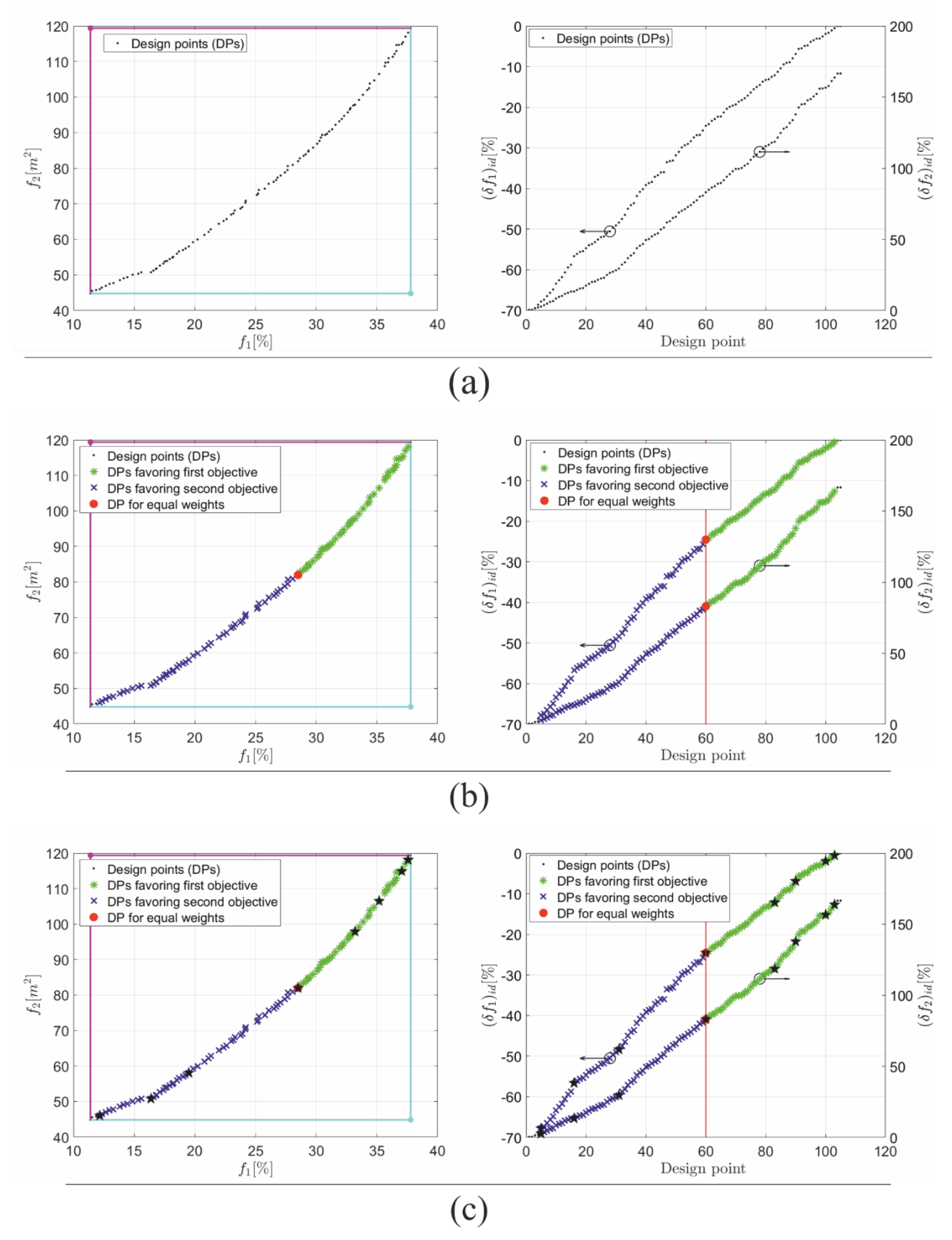
After running the program, two figures are displayed (see Figure 6a). The first one is a graph with the Pareto set points (Pareto front) which conventionally are called design points (DPs). To have a deeper insight into the individual DPs, the second figure shows a relative change between a certain i-th DP and the ideal solution for the first (left y-axis) and the second (right y-axis) objective function. By referring to the examined optimization problem in which the objectives are the benefit (the exergy efficiency η_ex) and the cost (the total heat transfer area A_tot) criteria, the corresponding relative changes can be defined as follows:

$${\left(\delta f_1\right)}_{id}=\frac{{\left(f_1\right)}_i-max\left(f_1\right)}{max\left(f_1\right)}·100\%$$

(27)

$${\left(\delta f_2\right)}_{id}=\frac{{\left(f_2\right)}_i-min\left(f_2\right)}{min\left(f_2\right)}·100\%$$

(28)

By convention, the relative changes defined in Equations (27) and (28) will be named as deviations from the ideal solution for easier identifying their meaning and intended use. Having defined index_min and index_max, the program will automatically adjust the appropriate formula for the other configurations of the objective function types (cost or benefit).

Next, the user decides what range of decision-making preferences is to be covered (question 1). Technically, it is done by introducing the preference range PR parameter which is used in place of the WS in Equation (25). By assigning a certain value to the PR, the program applies Equation (25) twice to generate two-weight distributions, i.e., one that favors the first objective and the equivalent one that is beneficial for the second criterion. As an example, assigning PR = 5.0 is equivalent to specifying the criteria weights as: w₁ = 0.9, w₂ = 0.1 and w₁ = 0.1, w₂ = 0.9. By applying the TOPSIS procedure, the design points corresponding to the selected weight distributions are indicated. Additionally, the design point calculated by assigning w₁ = 0.5, w₂ = 0.5 is highlighted as being the characteristic Pareto solution reflecting equal importance of the criteria. The solutions which are distributed between the equal weights point and design points indicated using PR parameter are graphically indicated (see Figure 6b) as solutions favoring the first and the second objective. The discussed step of the procedure can be perceived as being equivalent to deciding what range of criteria weights are to be considered [24,25]. In other words, by assigning a certain value to the PR parameter, the set of design points corresponding to the selected criteria weights is indicated.

In the next step, the user decides which objective function is a priority criterion (question 2). By simply assigning the value (1 or 2) to the priority function PF parameter, one of the criteria (f₁ or f₂) is selected as primary. Then, the user must decide to what extent the final design point should differ from the point of the equal weight (question 3). This is done by direct assigning a value to the WS parameter. As depicted in Figure 5, the choice is limited to the range between 1.0 and PR. In other words, the user cannot choose the design point which is out of the range covered by assigning PR a few steps earlier. As an example, by assigning PF = 1 and WS = 2.0, the criteria weights are specified as: w₁ = 0.6, w₂ = 0.4. To highlight graphically (see Figure 6c) the proposed design point, the TOPSIS is applied for the second time. Thereby, the WS parameter is used (after choosing the priority criterion by applying the PF parameter) for indicating a single, and potentially the final design point.

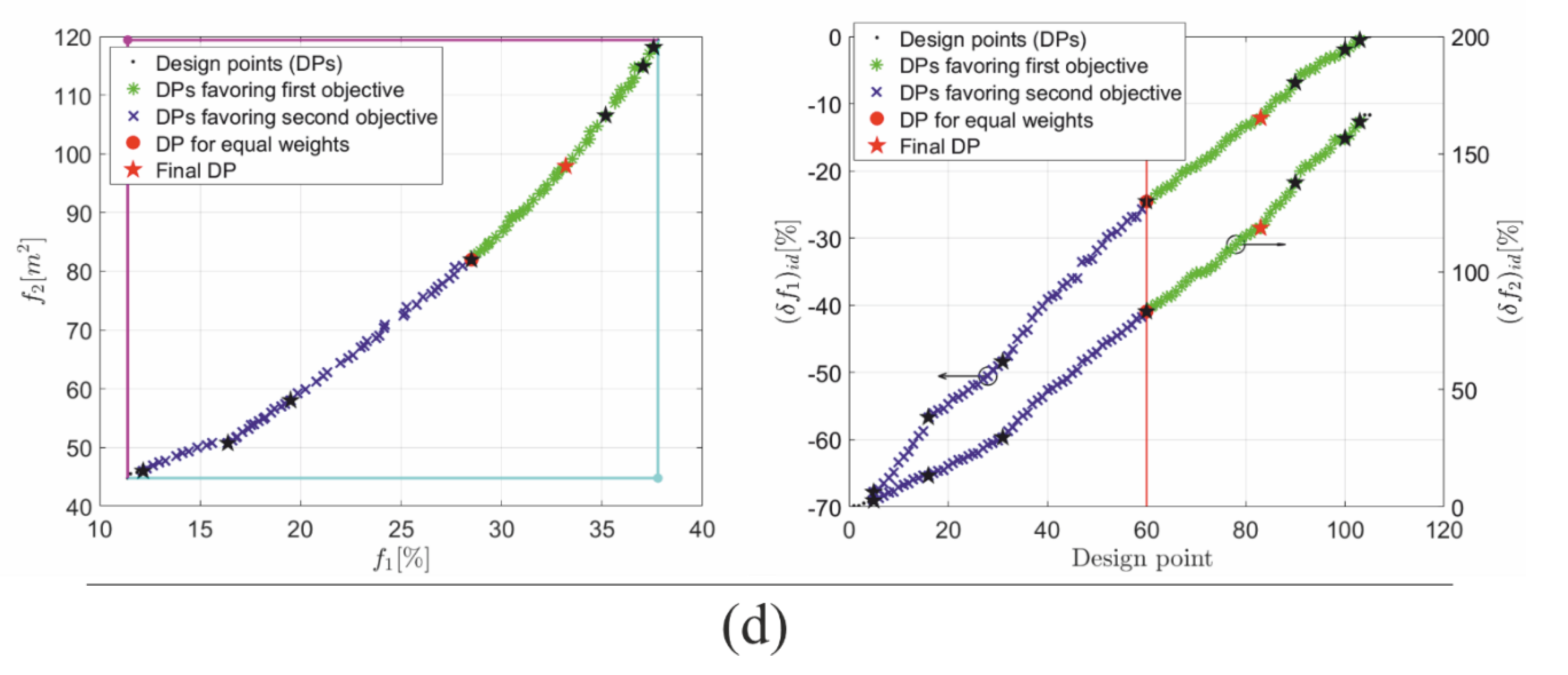
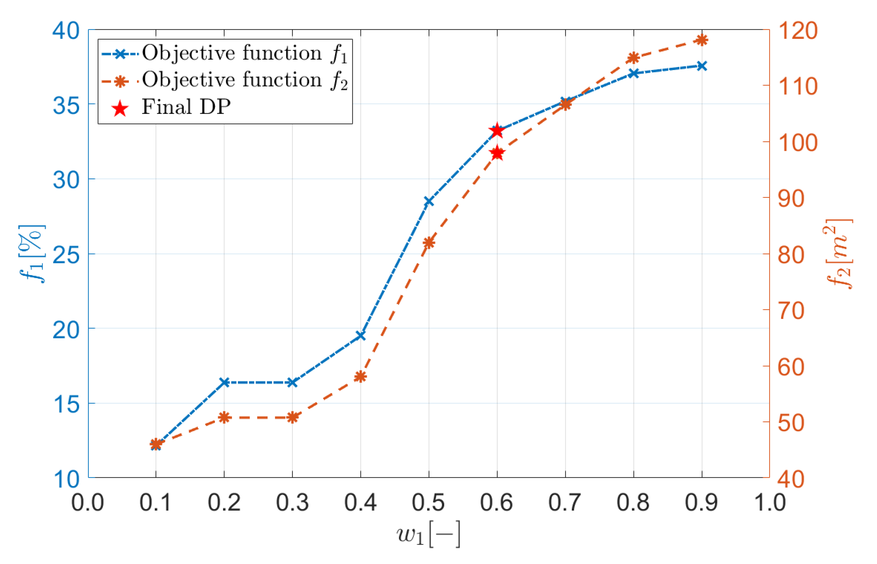
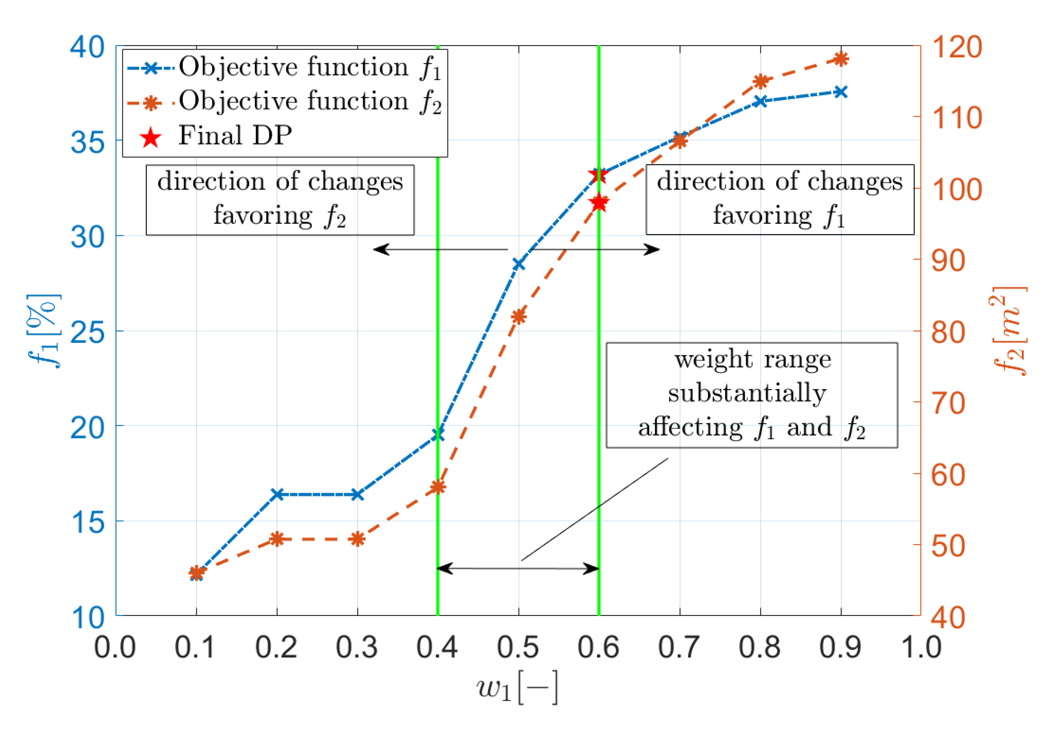
The user can decide whether to consider other design points or mark the last choice as the final solution (see Figure 6d). To provide deeper insight into the decisions taken, the graph depicted in Figure 7 is displayed. It presents the design points corresponding to various weights w₁ which were specified indirectly by assigning values to the PF and WS parameters. Obviously, for a certain value of the w₁, the weight distribution is fully defined since the second weight w₂ is calculated using Equation (26).

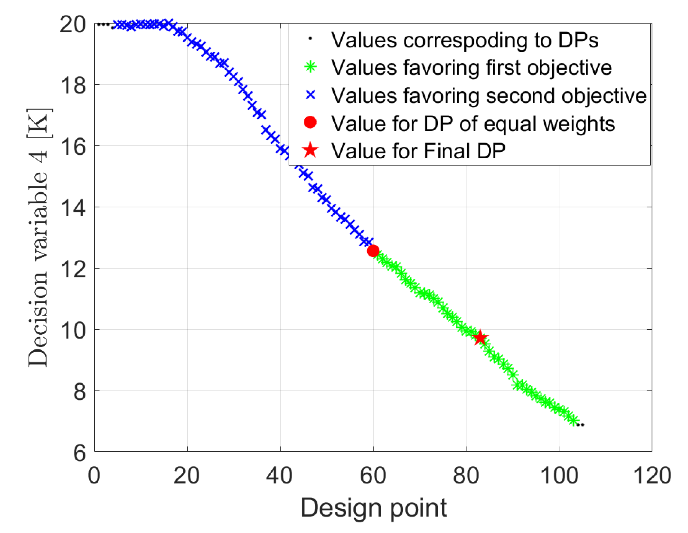
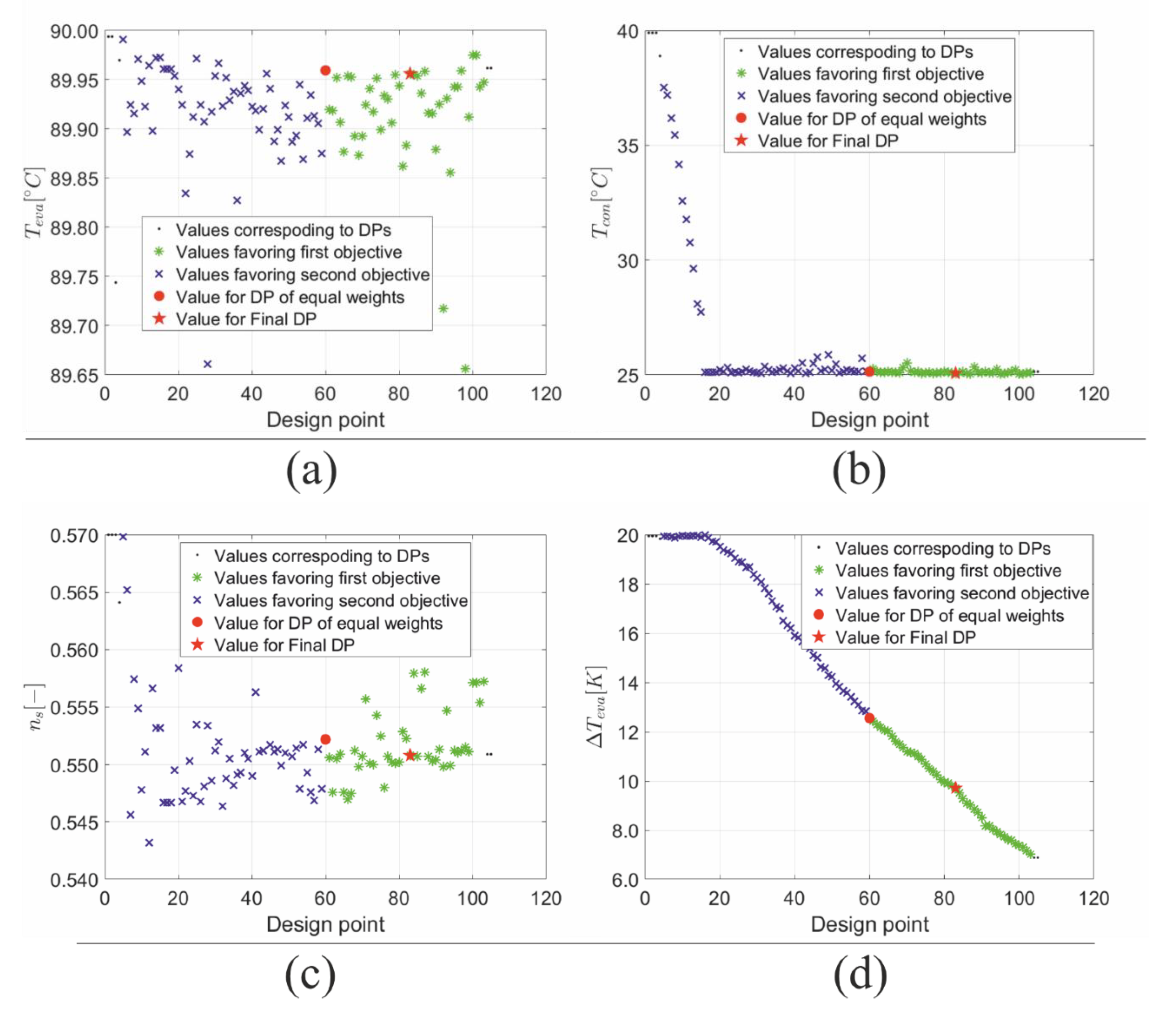
If the user opts for conducting the entire procedure from the beginning, the program will clear the marked points and the decision-making process will be repeated. If not, the procedure is completed. In the end, the program displays graphs with decision variable values corresponding to each design point. The decisions taken by the user are marked, indicating what values of the decision variables favor the examined objectives and what is the decision variable value corresponding to the final design point. As an example, the graph generated for one of the examined decision variables, i.e., the temperature difference ΔT_eva (see Figure 1b), is presented in Figure 8. Being the fourth element of a vector written in Equation (24), it is marked with a number 4.

5. Results and Discussion

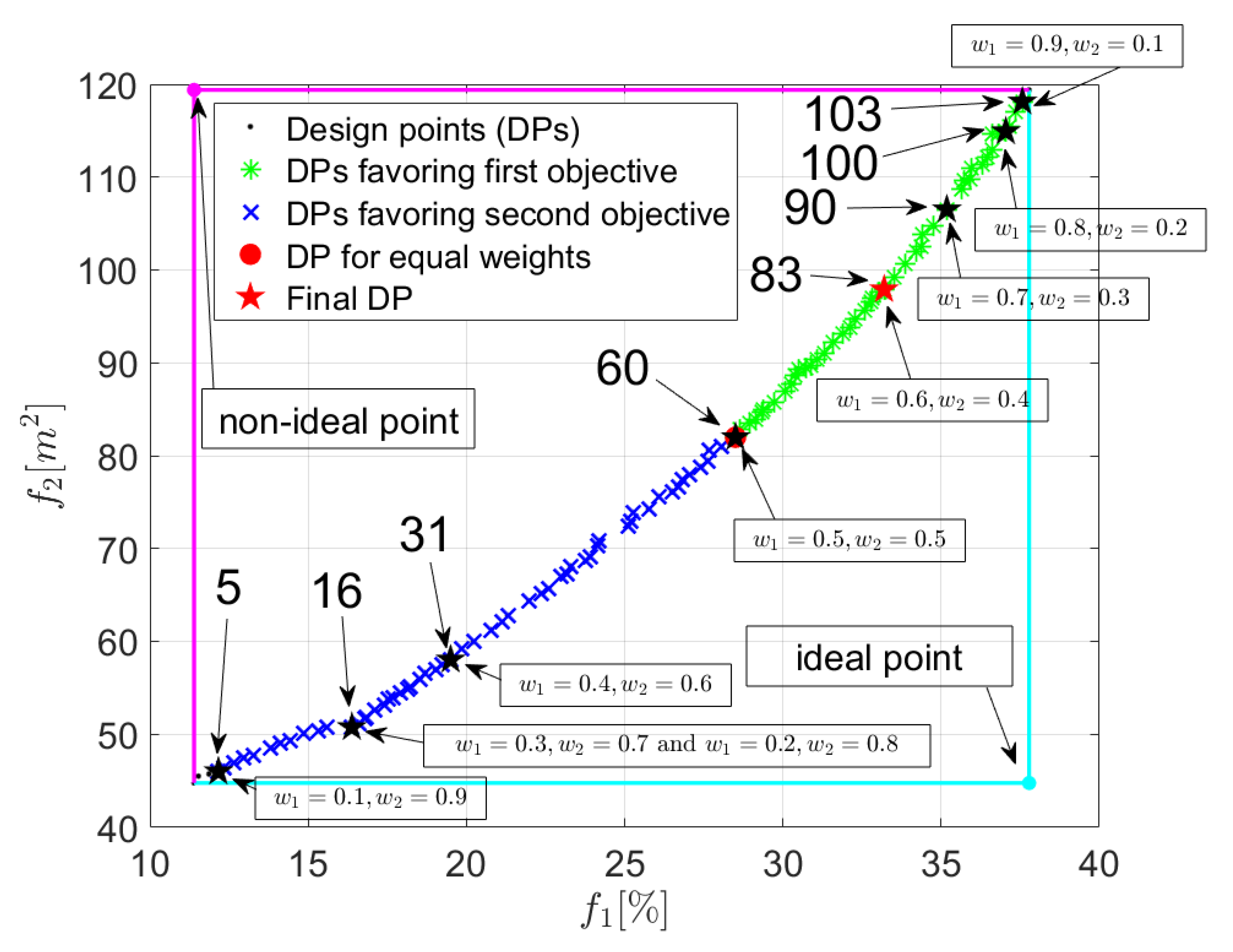
For a better understanding of the developed tool, an illustrative decision-making procedure applied for the results of bi-objective optimization is presented. As mentioned, the exergy efficiency η_ex (objective function f₁) and total heat transfer area A_tot (objective function f₂) were defined as the criteria optimizing the operation of the ORC power plant. The set of optimal design points generated by applying NSGA-II is depicted in Figure 9 (obtained for the salinity of geothermal water equaling 0.00 kgkg⁻¹, for more details, see [26]). At this stage, the designer of the ORC may choose one of the Pareto set points and consider it as the final solution. The description of this process by analyzing the data generated by the TRADeS is given below.

5.1. Decision-Making Analysis

Defining the preference range of design points. It was decided to assign a value of 5.0 to the preference range PR parameter. In other words, the marked solutions (see Figure 9) are indicated for the criteria weights with their numerical values between 0.1 and 0.9 (see

Table 2. Results of decision-making procedure.

Parameter	No. of WD	PR	PF	WS	w1	w2	No. of DP	f1	(δf1)id	f2	(δf2)id
unit	[-]	[-]	[-]	[-]	[-]	[-]	[-]	[%]	[%]	[m2]	[%]
value	1	5.0	1	5.0	0.9	0.1	103	37.6	−0.57	118	164
	2	5.0	1	4.0	0.8	0.2	100	37.0	−1.95	115	157
	3	5.0	1	3.0	0.7	0.3	90	35.2	−6.88	107	138
	4	5.0	1	2.0	0.6	0.4	83	33.2	−12.1	97.9	119
	5	5.0	1	1.0	0.5	0.5	60	28.5	−24.6	82.0	83.1
	6	5.0	2	2.0	0.4	0.6	31	19.5	−48.4	58.0	29.6
	7	5.0	2	3.0	0.3	0.7	16	16.4	−56.6	50.7	13.3
	8	5.0	2	4.0	0.2	0.8	16	16.4	−56.6	50.7	13.3
	9	5.0	2	5.0	0.1	0.9	5	12.2	−67.8	46.0	2.70

), similar to [25]. Based on this decision, the design points are divided into solutions favoring the first and the second criterion. The point corresponding to w₁ = 0.5, w₂ = 0.5 is indicated automatically and its role is to separate these solutions. The design points marked with the black dots are excluded from the analysis as solutions corresponding to weight distributions (WDs) which are out of the selected range.

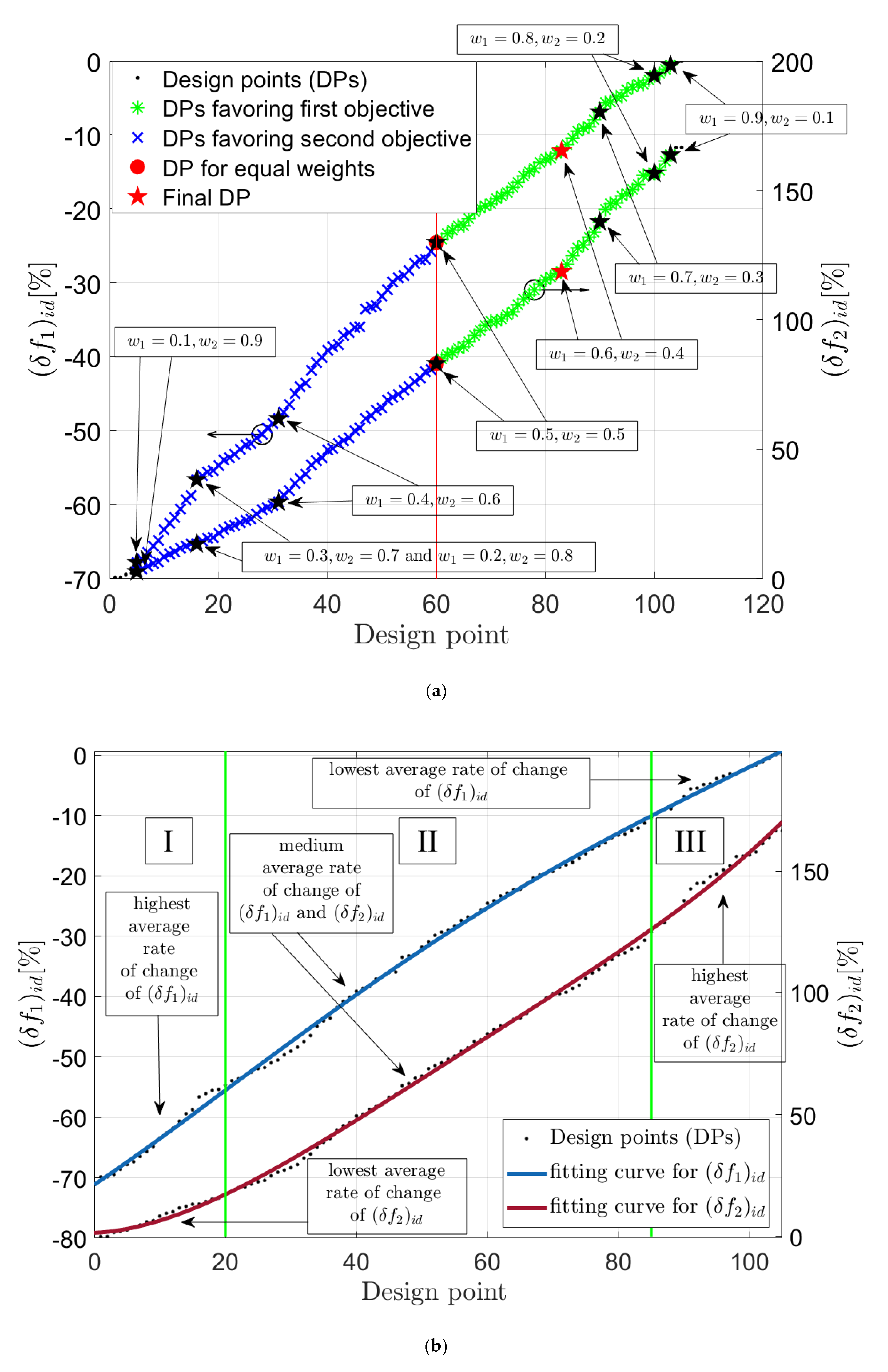
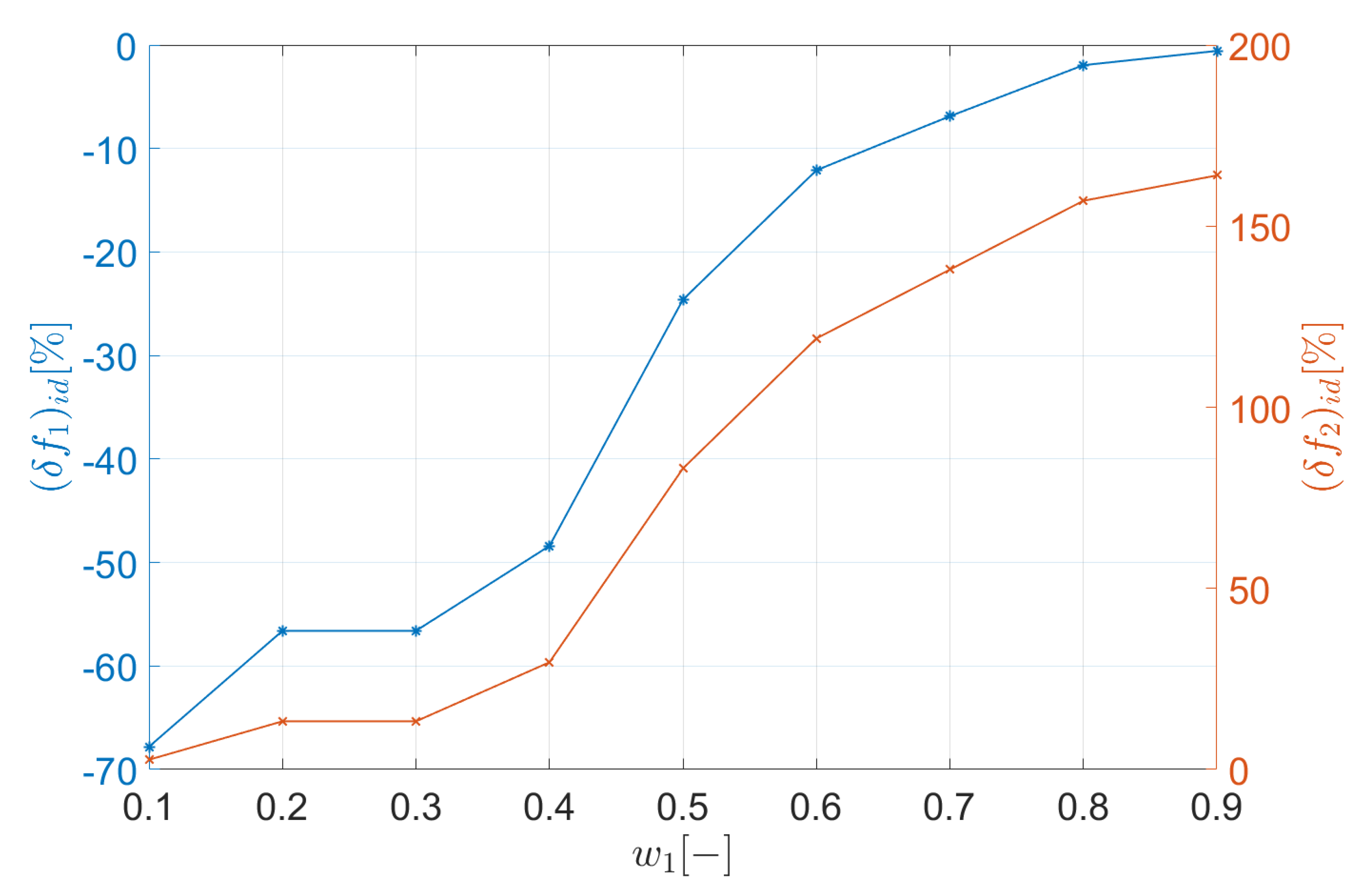
Examining weights’ influence on the selected design points. The design points marked with the black stars are selected based on the different values assigned to the prior function PF and weight superiority WS parameters (see Table 2). By analyzing the graphs depicted in Figure 10 and the outcomes listed in Table 2, it is noted that both objective functions f₁ and f₂ are very sensitive to weights in a range between 0.4 and 0.6. As an example, by changing the weight w₁ from 0.4 to 0.6, the deviation (δf₁)_id from the ideal solution of the exergy efficiency increased (towards (δf₁)_id = 0%) by 36.3 pp, while by increasing the w₁ from 0.6 to 0.8, the (δf₁)_id increased by only 10.2 pp. For a more detailed analysis of this relationship, the graph depicted in Figure 11 is examined. Specifically, the steepest slopes of the (δf₁)_id and (δf₂)_id are reported for the weights w₁ ranging between 0.4 and 0.6. Thereby, by increasing w₁, within the aforementioned range, a significant improvement in the exergy efficiency η_ex can be obtained. Similarly, by decreasing w₁, from 0.6 to 0.4, the total heat transfer area A_tot can be substantially reduced. Therefore, the decision-maker should keep in mind that the change of weights in the interval of 0.4 to 0.6 is associated with significant improvement of the first objective and substantial deterioration of the second one. For the remaining weight distributions (0.6 $<$ w₁ $\le$ 0.9 and 0.1 $\le$ w₁ $<$ 0.4), the objectives are less sensitive, or their numerical values do not change (see design point numbered as 16 in Figure 9).

From the user’s perspective, the discussed sensitivity of the solutions to the criteria weights can be easily identified by tracking the locations of design points marked on graphs presented in Figure 9 and Figure 10a. In particular, if the selected solutions are distributed close to each other, they are less sensitive to the assigned weights. For points located far from each other, an inverse relationship is observed, i.e., they are more sensitive to the selected weights.

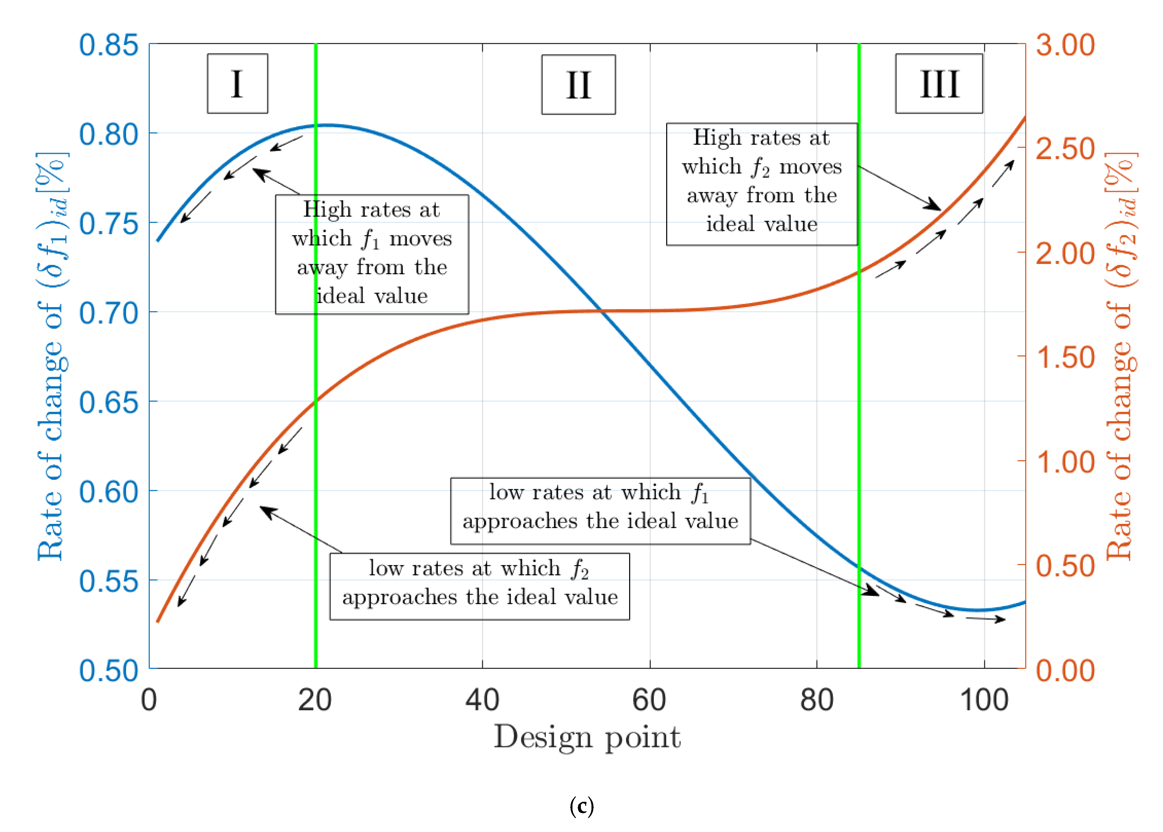
Excluding adverse design point regions. Another decision-making aspect which can be examined by applying the proposed approach relates to the rate at which the individual solutions of the objectives f₁ and f₂ change for different regions of design points. To obtain a more complete picture of the problem, the results presented as points in Figure 10a are approximated by the polynomial curves (see Figure 10b) using the Curve Fitting toolbox embedded in MATLAB software. It was assessed that the regions I and III correspond to the substantial difference of rates at which the objectives approach their ideal solutions. The assessment of which Pareto set points belong to which specific region is subjective. However, the decision is not made unreasonably, but it is based on a careful analysis which is explained in the following paragraphs.

As presented in

Table 3. Variability of the deviations from ideal solution over considered regions of design points.

	Average Rate of Change of the Deviations from Ideal Solution
	(δf1)id [%]	(δf2)id [%]
region I	0.78	0.82
region II	0.70	1.67
region III	0.54	2.21

, for region I, the highest average rate of change of the (δf₁)_id is combined with the lowest average rate of change of the (δf₂)_id. By following the direction in which (δf₂)_id approaches 0%, the above relationship means that a slight improvement of the objective f₂ is associated with a significant deterioration of the criterion f₁. By examining the results covering region III, an inverse relationship is reported, i.e., when the (δf₁)_id approaches 0%, a small beneficial increase in f₁ is combined with a substantial unfavorable increase in f₂. For this reason, the design points located in regions I and III are excluded, limiting the choice of the decision-maker to solutions covering the region II. Thereby, the weights $w_1\le 0.3$ and $w_1\ge 0.7$ (see Table 2), as values corresponding to design points which are placed in regions I and III, should not be considered for the selection of the final operating point.

For further investigating the effects described above, the instantaneous rates at which the objectives approach their ideal values were determined. This was done by calculating the first derivatives of the deviations (δf₁)_id and (δf₂)_id (presented in Figure 10b) with the design point as a variable. As depicted in Figure 10c, regions I and III are indeed the areas in which an intensified contradicting relation between the objectives is observed. Specifically, for region I, the low rates at which the objective f₂ approaches the ideal value, are combined with the high rates at which f₁ moves away from its ideal solution. Similarly, for region III, the low rates at which the objective f₁ approaches the ideal value, are associated with the high rates at which the f₂ moves away from its ideal solution. On the other hand, the design points covering region II are characterized by the intermediate rates at which the objectives approach/move away from their ideal values. Thereby, the design points located in region II may be associated with the most sustainable relation between deterioration and improvement of the criteria, while approaching the ideal value of one of them.

Technically, regions I and III can be perceived as sets of Pareto solutions similar to Pareto weak optimal points [43]. Considering such points, it is possible to improve/aggravate one of the objectives without changing the value of the other. For these cases, the rate of change of the deviation from the ideal solution would be equal to 0.00% for one of the objectives. As depicted in Figure 10c, the rates of the (δf₁)_id and (δf₂)_id are close to 0.00%, being less than 0.55% for the first criterion (region III) and less than 0.30% for the second objective (region I).

Summarizing, it should be noted that a discussed relationship between the objectives, emerging in regions strongly favoring one of the criteria, occurs in the case of the Pareto front convex to the ideal solution [44]. For the non-convex Pareto curves, the opposite relation would be observed. Specifically, by approaching the ideal value of the first objective, a significant improvement of this objective would be accompanied by a slight deterioration of the second criterion. For such regions, selecting design points that are closer to the ideal value of the first objective would be preferable. In practical applications, the non-convex shapes of the Pareto curves are considered less frequently [45], thereby making the above-mentioned recommendations applicable for the ORCs and other industrial systems.

Selecting the final design point. After an initial overview of the design points, the designer can choose the potential final optimal solution. Since the size of the system is usually not as important as the power capacity for the geothermal ORC, it was decided to favor the first objective (PF = 1) with the WS parameter equaling 2.0 which is equivalent to the w₁ = 0.6, w₂ = 0.4 weight distribution.

Overview of the considered design points with respect to weights. By negating the selection of other design points, the user is directed to the next decision-making step. For deeper identifying the decisions taken, the results depicted in Figure 12 are examined. The considered design points are presented with respect to the selected weights w₁. As in the case of the graph shown in Figure 11, it is seen that the objective functions are very sensitive to weights in a range between 0.4 and 0.6. Therefore, a detailed analysis of the impact of the weight on the objectives is provided, thus satisfying one of the requisites of the robust decision-making process [46].

Restarting/ending the decision-making process. At this stage, the designer can opt for reconsidering the weight distributions and thereby analyzing new solutions, including the final design point. For the studied case, it was decided not to consider other distributions of the potential design points, thus ending the decision-making process.

Analysis of the decisions taken with respect to decision variables. The graphs which complete the entire procedure are presented in Figure 13. The final decisions taken by the user are marked on scatter distribution graphs which are generated for each decision variable of the examined optimization problem.

Taking into consideration the bounds specified in Equations (12) and (14), it can be stated that the evaporation temperature T_eva (see Figure 13a) and specific speed n_s (see Figure 13c) are distributed in a narrow range. Specifically, the T_eva values close to 90 °C are reported as optimal, while for the n_s most outcomes are hovering around 0.55. For this reason, it is not possible to divide the obtained outcomes into values favoring the first (η_ex) or the second (A_tot) objective. In the case of the condensation temperature T_con (see Figure 13b), it is clear that the values close to 40 °C (upper bound, see Equation (13)) favor the second criterion, while the values close to 25 °C (lower bound, see Equation (13)) are beneficial for the first objective. However, most of the solutions (favoring both f₁ and f₂) are obtained for 25 °C. As seen in Figure 13d, the temperature difference ΔT_eva is monotonically decreasing with respect to design points and the values closer to 20 K (upper bound, see Equation (15)) are beneficial for the second objective, while the values closer to ~6 K are favorable the first criterion.

Summarizing, the graphs depicted in Figure 13 are complementary to the decision-making procedure. Even though they do not affect the decision-making process itself, they provide information as to what values of the decision variables correspond to the final design point and what ranges of these parameters favor the individual objectives.

5.2. Comparative Analysis with other Decision-Making Methods

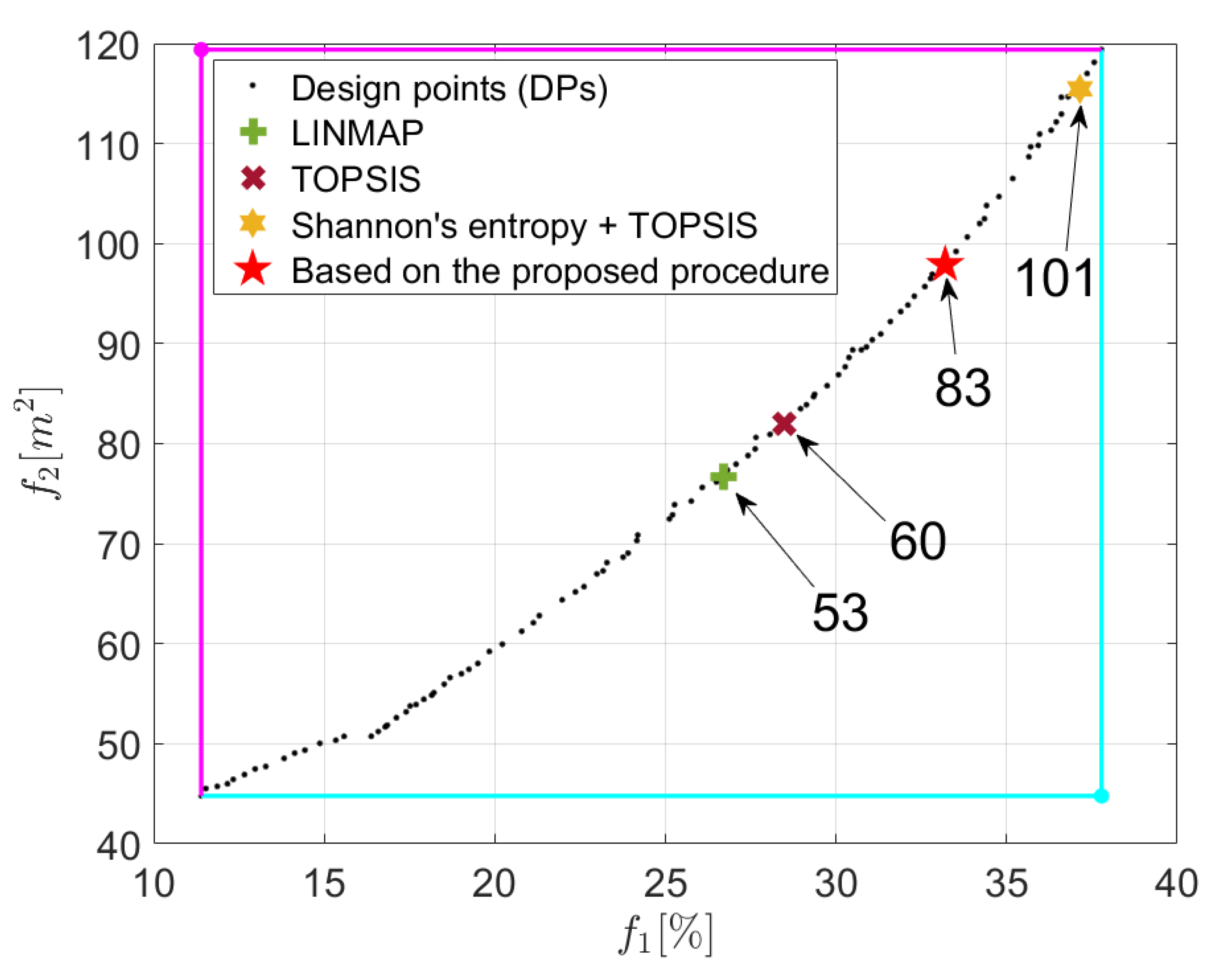
The design point selected using the proposed procedure is marked along with solutions indicated by applying well-established decision-making approaches (see Figure 14). As mentioned in the Introduction, the LINMAP technique is based on the assumption that the Pareto set point which has the shortest distance from the ideal point is the best candidate for the final solution. Similarly, by applying the TOPSIS approach, the design point which has the shortest distance from the ideal point and the longest distance from the non-ideal point is considered as the definitive choice. As discussed previously, the scholars utilizing these techniques rarely took the opportunity to specify the decision-making “preferences” by assigning weights to the criteria. Having analyzed the LINMAP or TOPSIS calculation procedure, it is clear that omitting this step is equivalent to specifying an equal importance of the objectives by implicitly assigning w₁ = 1.0 and w₂ = 1.0. The design points indicated by applying this approach for the LINMAP and TOPSIS techniques are numbered as 53 and 60, respectively.

If one decides to specify the preferences with respect to the optimization criteria, one can opt for the subjective or objective methods for assigning weights. An application of the objective approach is illustrated in Figure 14. Specifically, the design point numbered as 101 is indicated by employing the TOPSIS technique combined with Shannon’s entropy method. The latter was applied for determining the criteria weights. The detailed description of Shannon’s entropy procedure can be found in [23]. With regard to the design point numbered as 83, it was determined by applying the developed decision-making tool. As already discussed, the proposed procedure is based on the application of the TOPSIS technique. However, the criteria weights are determined subjectively based on the detailed analysis described in the decision-making process. Thereby, the proposed approach is not solely based on the mathematically defined procedures, making the selection of the final operating point a more conscious and comprehensible process.

In the “Decision-making process” section, it was suggested that the final design point should be located in a range between 20 and 85 design point (see Figure 10b). As seen in Figure 14, the solutions obtained using the LINMAP and TOPSIS procedures are located inside the suggested region (in region II), whereas the design point indicated by applying the Shannon’s entropy + TOPSIS approach is placed out of the acceptable range (in region III). The choice of design points belonging to the region III was not recommended since, in that range of solutions, an intensified adverse relationship between the objectives was reported.

The unquestionable advantage of the examined approaches (LINMAP, TOPSIS, Shannon’s entropy + TOPSIS) is a simple structure and fast indication of the final design point for the examined system. These features make them particularly useful for inexperienced decision-makers. The tool developed in this study allows for conducting a more comprehensive decision-making process, providing the opportunity for specifying the decision-maker preferences, tracking the decisions taken and analyzing the results of the procedure.

6. Conclusions

This study aimed to propose a decision-making tool (called TRADeS) for a bi-objective optimization of the geothermal ORC power plant. By maximizing the exergy efficiency and minimizing the total heat transfer area, the Pareto set of optimal design points was determined. To conduct an in-depth decision-making study and select the final optimal solution, the developed tool was utilized. A thorough analysis which was performed by examining the data generated by created software allowed to draw the following conclusions:

• while analyzing the rates at which the criteria approach their ideal solutions, it was found that there are regions of design points in which an intensified deterioration of one of the objectives is combined with a slight improvement of the second criterion. For this reason, from among the 105 design points, these numbered as lower than 20 and higher than 85 have been excluded from the set of potential final design points;
• while considering the final design point, it was highlighted to discard the weights $w_1\ge 0.7$ and $w_1\le 0.3$ as values corresponding to excluded Pareto set points;
• most commonly applied forms of decision-making techniques, such as LINMAP or TOPSIS, are appropriate for inexperienced designers as they do not require specifying the decision-maker preferences. As a tool allowing for a careful examination of the criteria weights, the proposed program provides a more conscious and comprehensible choice of the final optimal configuration for the examined system.

The tool which was developed in this study should be perceived as a useful decision-making support for practical bi-objective optimization problems. By using the software and implementing the proposed recommendations, a more detailed analysis of the Pareto solutions is provided, giving a deeper insight into the decision-making process and selection of the final design point. Simultaneously, intuitive operation and generic structure allow for applying the tool in other industrial applications.

References

1. Altun, A.F.; Kilic, M. Thermodynamic performance evaluation of a geothermal ORC power plant. Renew. Energy 2020, 148, 261–274. [Google Scholar] [CrossRef]
2. Roumpedakis, T.C.; Loumpardis, G.; Monokrousou, E.; Braimakis, K.; Charalampidis, A.; Karellas, S. Exergetic and economic analysis of a solar driven small scale ORC. Renew. Energy 2020, 157, 1008–1024. [Google Scholar] [CrossRef]
3. Kalina, J.; Świerzewski, M.; Strzałka, R. Operational experiences of municipal heating plants with biomass-fired ORC cogeneration units. Energy Convers. Manag. 2019, 181, 544–561. [Google Scholar] [CrossRef]
4. Wang, L.; Bu, X.; Li, H. Multi-objective optimization and off-design evaluation of organic rankine cycle (ORC) for low-grade waste heat recovery. Energy 2020, 203, 117809. [Google Scholar] [CrossRef]
5. Kosmadakis, G.; Neofytou, P. Investigating the performance and cost effects of nanorefrigerants in a low-temperature ORC unit for waste heat recovery. Energy 2020, 204, 117966. [Google Scholar] [CrossRef]
6. Sadreddini, A.; Ashjari, M.A.; Fani, M.; Mohammadi, A. Thermodynamic analysis of a new cascade ORC and transcritical CO2 cycle to recover energy from medium temperature heat source and liquefied natural gas. Energy Convers. Manag. 2018, 167, 9–20. [Google Scholar] [CrossRef]
7. Hu, S.; Li, J.; Yang, F.; Yang, Z.; Duan, Y. Multi-objective optimization of organic Rankine cycle using hydrofluorolefins (HFOs) based on different target preferences. Energy 2020, 203, 117848. [Google Scholar] [CrossRef]
8. Dai, X.; Shi, L.; An, Q.; Qian, W. Screening of hydrocarbons as supercritical ORCs working fluids by thermal stability. Energy Convers. Manag. 2016, 126, 632–637. [Google Scholar] [CrossRef]
9. Oyekale, J.; Haberle, F.; Petrollese, M.; Brüggemann, D.; Cau, G. Thermo-economic evaluation of actively selected siloxane mixtures in a hybrid solar-biomass organic Rankine cycle power plant. Appl. Therm. Eng. 2020, 165, 114607. [Google Scholar] [CrossRef]
10. Feng, Y.; Hung, T.; Zhang, Y.; Li, B.; Yang, J.; Shi, Y. Performance comparison of low-grade ORCs (organic Rankine cycles) using R245fa, pentane and their mixtures based on the thermoeconomic multi-objective optimization and decision makings. Energy 2015, 93, 2018–2029. [Google Scholar] [CrossRef]
11. Srinivasan, V.; Shocker, A. Linear programming techniques for multidimensional analysis of preference. Psychometrica 1973, 38, 337–369. [Google Scholar] [CrossRef]
12. Hwang, C.L.; Yoon, K.P. Multiple Attributes Decision making Methods and Applications; Springer: Berlin/Heidelberg, Germany, 1981. [Google Scholar]
13. Feng, Y.; Zhang, Y.; Li, B.; Yang, J.; Shi, Y. Sensitivity analysis and thermoeconomic comparison of ORCs (organic Rankine cycles) for low temperature waste heat recovery. Energy 2015, 82, 664–677. [Google Scholar] [CrossRef]
14. Behzadi, A.; Arabkoohsar, A.; Gholamian, E. Multi-criteria optimization of a biomass-fired proton exchange membrane fuel cell integrated with organic rankine cycle/thermoelectric generator using different gasification agents. Energy 2020, 201, 117640. [Google Scholar] [CrossRef]
15. Oyekale, J.; Petrollese, M.; Cau, G. Multi-objective thermo-economic optimization of biomass retrofit for an existing solar organic Rankine cycle power plant based on NSGA-II. Energy Rep. 2020, 6, 136–145. [Google Scholar] [CrossRef]
16. Wu, Z.; Zhang, Y.; Sheng, Y. Energy, exergy, economic (3E) analysis and multi-objective optimization of a novel dual functional integration system. Energy Convers. Manag. 2019, 199, 111962. [Google Scholar] [CrossRef]
17. Pourrahmani, H.; Moghimi, M. Exergoeconomic analysis and multi-objective optimization of a novel continuous solar-driven hydrogen production system assisted by phase change material thermal storage system. Energy 2019, 189, 116170. [Google Scholar] [CrossRef]
18. Shen, G.; Yuan, F.; Li, Y.; Liu, W. The energy flow method for modeling and optimization of Organic Rankine Cycle (ORC) systems. Energy Convers. Manag. 2019, 199, 111958. [Google Scholar] [CrossRef]
19. Wang, Z.; Hu, Y.; Xia, X.; Zuo, Q.; Zhao, B.; Li, Z. Thermo-economic selection criteria of working fluid used in dual-loop ORC for engine waste heat recovery by multi-objective optimization. Energy 2020, 197, 117053. [Google Scholar] [CrossRef]
20. Shao, M.; Han, Z.; Sun, J.; Xiao, C.; Zhang, S.; Zhao, Y. Review of multi-criteria decision making applications for renewable energy site selection. Renew. Energy 2020, 157, 377–403. [Google Scholar] [CrossRef]
21. Odu, G.O. Weighting Methods for Multi-Criteria Decision Making Technique. J. Appl. Sci. Environ. Manag. 2019, 23, 1449–1457. [Google Scholar] [CrossRef] [Green Version]
22. Bina, S.M.; Jalilinasrabady, S.; Fujii, H. Thermo-economic evaluation of various bottoming ORCs for geothermal power plant, determination of optimum cycle for Sabalan power plant exhaust. Geothermics 2017, 70, 181–191. [Google Scholar] [CrossRef]
23. Shannon, C.E. A mathematical theory of communication. SIGMOBILE Mob. Comput. Commun. Rev. 2001, 5, 3–55. [Google Scholar] [CrossRef]
24. Wang, L.; Li, H.; Bu, X. Multi-objective optimization of Binary Flashing Cycle (BFC) driven by geothermal energy. Appl. Therm. Eng. 2020, 166, 114693. [Google Scholar] [CrossRef]
25. Detchusananard, T.; Sharma, S.; Maréchal, F.; Arpornwichanop, A. Generation and selection of Pareto-optimal solution for the sorption enhanced steam biomass gasification system with solid oxide fuel cell. Energy Convers. Manag. 2019, 196, 1420–1432. [Google Scholar] [CrossRef]
26. Jankowski, M.; Borsukiewicz, A.; Wiśniewski, S.; Hooman, K. Multi-objective analysis of an influence of a geothermal water salinity on optimal operating parameters in low-temperature ORC power plant. Energy 2020, 202, 117666. [Google Scholar] [CrossRef]
27. Da Lio, L.; Manete, G.; Lazzaretto, A. A Mean-line model to predict the design efficiency of radial inflow turbines in organic Rankine cycle (ORC) systems. Appl. Energy 2017, 205, 187–209. [Google Scholar] [CrossRef]
28. Whitfield, A.; Baines, N.C. Design of Radial Turbomachines; Longman Scientific & Technical: New York, NY, USA, 1990. [Google Scholar]
29. Aungier, R.H. Turbine Aerodynamics; ASME Press: New York, NY, USA, 2006. [Google Scholar]
30. Fiaschi, D.; Manfrida, G.; Maraschiello, F. Design and performance prediction of radial ORC turboexpanders. Appl. Energy 2015, 138, 517–532. [Google Scholar] [CrossRef]
31. Bekiloğlu, H.E.; Bedir, H.; Anlaş, G. Multi-objective optimization of ORC parameters and selection of working fluid using preliminary radial inflow turbine design. Energy Convers. Manag. 2019, 183, 833–847. [Google Scholar] [CrossRef]
32. Gullapalli, V.S. Modeling of brazed plate heat exchangers for ORC systems. Energy Procedia 2017, 129, 443–450. [Google Scholar] [CrossRef]
33. Li, J.; Ge, Z.; Duan, Y.; Yang, Z.; Liu, Q. Parametric optimization and thermodynamic performance comparison of single-pressure and dual-pressure evaporation organic Rankine cycles. Appl. Energy 2018, 217, 409–421. [Google Scholar] [CrossRef]
34. The MathWorks Inc. MATLAB, version R2019a; The MathWorks Inc.: Natick, MA, USA, 2019. [Google Scholar]
35. Lemmon, E.W.; Huber, M.L.; McLinden, M.O. Reference Thermodynamic and Transport Properties—Refprop NIST Standard Reference Base 23, version 9.1; NIST: Gaithersburg, MD, USA, 2013.
36. Bahadormanesh, N.; Rahat, S.; Yarali, M. Constrained multi-objective optimization of radial expanders in organic Rankine cycles by firefly algorithm. Energy Convers. Manag. 2017, 148, 1179–1193. [Google Scholar] [CrossRef]
37. Jankowski, M.; Borsukiewicz, A. A Novel Exergy Indicator for Maximizng Energy Utilization in Low-Temperature ORC. Energies 2020, 13, 1598. [Google Scholar] [CrossRef] [Green Version]
38. Tomków, Ł.; Cholewiński, M. Modelling of a novel power-generating cycle for the utilization of the cold exergy of liquid natural gas with the adjustable parameters of working fluid. Energy Convers. Manag. 2019, 201, 112178. [Google Scholar] [CrossRef]
39. Li, P.; Han, Z.; Jia, X.; Mei, Z.; Han, X.; Wang, Z. Analysis and comparison on thermodynamic and economic performances of an organic Rankine cycle with constant and one-dimensional dynamic turbine efficiency. Energy Convers. Manag. 2019, 180, 665–679. [Google Scholar] [CrossRef]
40. Jankowski, M.; Borsukiewicz, A.; Szopik-Depczyńska, K.; Ioppolo, G. Determination of an optimal pinch point temperature difference interval in ORC power plant using multi-objective approach. J. Clean Prod. 2019, 217, 798–807. [Google Scholar] [CrossRef]
41. Deb, K.; Pratap, A.; Agarwal, S.; Meyarivan, T. A Fast and Elitist Multiobjective Genetic Algorithm: NSGA-II. IEEE Trans. Evol. Comput. 2002, 6, 182–197. [Google Scholar] [CrossRef] [Green Version]
42. Jankowski, M.; Borsukiewicz, A. Multi-objective approach for determination of optimal operating parameters in low-temperature ORC power plant. Energy Convers. Manag. 2019, 200, 112075. [Google Scholar] [CrossRef]
43. Chang, K.-H. Design Theory and Methods Using CAD/CAE; Elsevier Academic Press: Cambridge, MA, USA, 2014. [Google Scholar]
44. Wang, M.; Jing, R.; Zhang, H.; Meng, C.; Li, N.; Zhao, Y. An innovative Organic Rankine Cycle (ORC) based on Ocean Thermal Energy Conversion (OTEC) system with performance simulation and multi-objective optimization. Appl. Therm. Eng. 2018, 145, 743–754. [Google Scholar] [CrossRef]
45. Arora, J.S. Introduction to Optimum Design; Elsevier Academic Press: Cambridge, MA, USA, 2004. [Google Scholar]
46. Greco, S.; Ehrgott, M.; Figueira, J.R. (Eds.) Multiple Criteria Decision Analysis; Springer: New York, NY, USA; Berlin/Heidelberg, Germany; Dordrecht, The Netherlands; London, UK, 2016. [Google Scholar]
Figure 1. (a)—organic Rankine cycle (ORC) system architecture (b)—T-s diagram with ORC and simplified temperature distributions of geothermal and cold water [26].
Energies 13 05280 g001
Figure 2. Geometry and modeling of system components: (a)—vapor generator, (b)—turbine, (c)—condenser [26].
Energies 13 05280 g002aEnergies 13 05280 g002b
Figure 3. Flowchart of calculation steps.
Energies 13 05280 g003
Figure 4. Criterion weight as a function of weight superiority parameter.
Energies 13 05280 g004
Figure 5. Flowchart of the proposed decision-making procedure.
Energies 13 05280 g005
Figure 6. Graphs generated by the proposed decision-making tool: (a)—Pareto front and double y-axis graph, (b)—covering the decision-making preferences, (c)—marking the proposed design points, (d)—marking the final design point.
Energies 13 05280 g006aEnergies 13 05280 g006b
Figure 7. Values of the objective functions for selected weight distributions.
Energies 13 05280 g007
Figure 8. Graph generated at the end of the decision-making process: scatter distribution of the decision variable with marked decisions.
Energies 13 05280 g008
Figure 9. Pareto front with marked design points.
Energies 13 05280 g009
Figure 10. (a)—Deviations from ideal solutions for both objectives, (b)—Variability of deviations from ideal solution for different regions (I, II, III) of design points (c)—Rates at which the criteria approach/move away from their ideal solution.
Energies 13 05280 g010aEnergies 13 05280 g010b
Figure 11. Deviations from an ideal solution for different sets of weights.
Energies 13 05280 g011
Figure 12. Sensitivity analysis of criteria with respect to weight distributions.
Energies 13 05280 g012
Figure 13. Scatter distribution graphs for the examined decision variables: (a)—evaporation temperature Teva, (b)—condensation temperature Tcon, (c)—specific speed ns, (d)—temperature difference ΔTeva.
Energies 13 05280 g013
Figure 14. Design points indicated applying different decision-making approaches.
Energies 13 05280 g014