Abstract
This study uses an optimization approach representation and numerical solution for the variable viscosity and non-linear Boussinesq effects on the free convection over a vertical truncated cone in porous media. The surface of the vertical truncated cone is maintained at uniform wall temperature and uniform wall concentration (UWT/UWC). The viscosity of the fluid varies inversely to a linear function of the temperature. The partial differential equation is transformed into a non-similar equation and solved by Keller box method (KBM). Compared with previously published articles, the results are considered to be very consistent. Numerical results for the local Nusselt number and local Sherwood number with the six parameters (1) dimensionless streamwise coordinate ξ, (2) buoyancy ratio N, (3) Lewis number Le, (4) viscosity-variation parameter , (5) non-linear temperature parameter , and (6) non-linear concentration parameter are expressed in figures and tables. The Taguchi method was used to predict the best point of the maxima of the local Nusselt (Sherwood) number of 3.8636 (5.1156), resulting in ξ (4), N (10), Le (0.5), (−2), (2), (2) and ξ (4), N (10), Le (2), (−2), (2), (2), respectively.
1. Introduction
The coupled heat and mass transfer of free convection in saturated porous media have many important applications in nature and engineering. Examples include geothermal flow, nuclear waste storage, electronic heat transfer systems, building insulation, powder metallurgy, groundwater contamination, osmotic cooling and chemical industry separation procedures.
Cheng et al. [1] analyzed natural convection of a Darcian fluid about a cone. With respect to the study on heat and mass transfer, the coupled heat and mass transfer by free convection over a truncated cone in porous media, variable wall temperature and variable wall concentration (VWT/VWC) or variable heat flux and variable mass flux (VHF/VMF) was solved by Yih [2]. Cheng [3] considered an integral approach for heat and mass transfer by natural convection from truncated cones in porous media with variable wall temperature and concentration. Cheng [4] extended the work of Yih [2] and Cheng [3] to present Soret and Dufour effects on heat and mass transfer by natural convection from a vertical truncated cone in a fluid-saturated porous medium with variable wall temperature and concentration. Free convection from a truncated cone subject to constant wall heat flux in a micropolar fluid has been explored by Postelnicu [5]. Chamkha [6] considered coupled heat and mass transfer by MHD natural convection of micropolar fluid about a truncated cone in the presence of radiation and chemical reaction. Yih and Huang [7] investigated the effect of internal heat generation on free convection flow of non-Newtonian fluids over a vertical truncated cone in porous media: VWT/VWC. Cheng [8] solved free convection of a nanofluid about a vertical truncated cone. Amanulla et al. [9] explored thermal and momentum slip effects on hydromagnetic convection flow of a Williamson fluid past a vertical truncated cone. Mahdy [10] presented modeling of gyrotactic microorganisms non-Newtonian nanofluids due to free convection flow past a vertical porous truncated cone.
The study of the variable viscosity in porous media has been widely discussed. Lai and Kulacki [11] considered the effect of variable viscosity on convective heat transfer along a vertical surface in a saturated porous medium. Mahdy et al. [12] reported double-diffusive convection with variable viscosity from a vertical truncated cone in porous media in the presence of magnetic field and radiation effects. The effect of chemical reaction and heat generation or absorption on double-diffusive convection from a vertical truncated cone in porous media with variable viscosity was studied by Mahdy [13]. Vajravelu et al. [14] analyzed free convection boundary layer flow past a vertical surface in a porous medium with temperature-dependent properties.
The non-linear Boussinesq approximation has been the subject of much research. Vajravelu et al. [14] obtained solutions for a class of coupled nonlinear differential equations, arising in free convection flow at a vertical flat plate embedded in a saturated porous medium at high Reynolds numbers in the presence of heat sources (or sinks) and with non-linear density temperature variation. Prasad et al. [15] used the non-Darcy model and the non-Boussinesq approximation to explore free convection boundary layer flow past a vertical surface in a porous medium with temperature-dependent properties. With respect to heat and mass transfer, Kameswaran [16] examined the thermophoretic and non-linear convection in non-Darcy porous medium. Combined convection from a wavy surface embedded in a thermally stratified nanofluid saturated porous medium with non-linear Boussinesq approximation was analyzed by Kameswaran et al. [17]. The non-linear Boussinesq article for the case of truncated cone is lacking.
However, there are still very few instances of the Taguchi method being used to find the maximum values by simulation. Ho et al. [18] suggested adaptive network-based fuzzy inference system for prediction of surface roughness in the end milling process using hybrid Taguchi-genetic learning algorithm. Chou [19] studied optimization methods and examples. Taguchi optimization of bismuth-telluride-based thermoelectric cooler was examined by Kishore et al. [20]. Li and Kao [21] found Taguchi optimization of solar thermal and heat pump combi-systems under five distinct climatic conditions.
In this exploration, the Taguchi method and the numerical simulation of variable viscosity and non-linear Boussinesq effects on natural convection over a vertical truncated cone in porous media are investigated. To the best of our knowledge, this problem has not been investigated before. The partial differential equations are transformed into non-similar equations and solved using the Keller box method (KBM) proposed by Cebeci and Bradshaw [22]. The numerical simulation of six different parameters is carried out to obtain the maximum value of the local Nusselt (Sherwood) number and find the best parameter ratio. The study is divided into two phases: the first phase of the data is compared with the previously published article, the results are considered very consistent. The main parameters on the local Nusselt (Sherwood) number are presented in graphic and tabular form. The second stage uses the Taguchi method to optimize the six parameters of the local Nusselt (Sherwood) number. The larger the local Nusselt (Sherwood) number, the greater the amount of heat (mass) that is taken away from the cone.
2. Methods
2.1. Mathematical Equations
Phase 1: consider the influence of the variable viscosity and non-linear Boussinesq effects on the heat and mass transfer by free convection flow over a vertical truncated cone embedded in a saturated porous medium. Figure 1 shows the concept map. The boundary conditions are uniform wall temperature Tw and uniform wall concentration (UWT/UWC).
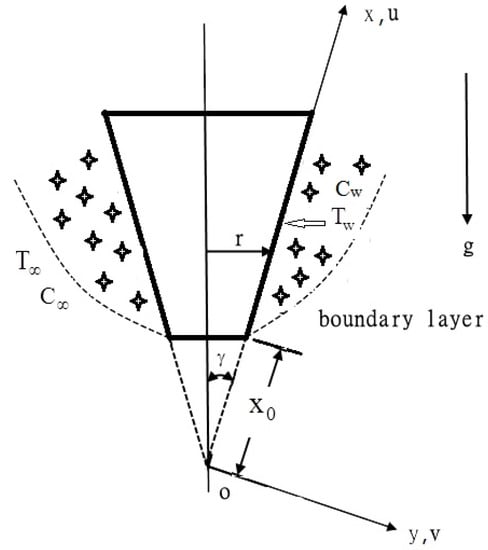
Figure 1.
Flow model and physical coordinate system.
The origin of the coordinate system is placed at the vertex of the full cone, where x is the coordinate along the surface of cone measured from the origin and y is coordinate normal to the surface, respectively. r is the local radius of the vertical truncated cone. is the half angle of the truncated cone. is the distance of the leading edge of the vertical truncated cone measured from the origin. All the fluid properties are assumed to be constant, except for the viscosity of fluid and the density variation in the buoyancy term. The viscosity of the fluid-saturated porous medium depends on the temperature T in the following form (refer Lai and Kulacki [11] and Vajravelu et al. [23]):
where γ is a viscosity-variation constant and is the viscosity of the ambient fluid with the following relation
Both a and are constants and their values depend on the reference state and the thermal property of the fluid, i.e., γ. In general, a > 0 (γ > 0) for liquid and a < 0 (γ < 0) for gas. The viscosity of the fluid usually reduces with increasing temperature while it enhances for gas.
To further show the appropriateness of Equation (1), correlations between viscosity and temperature for air and water are given below because these two are the most common working fluids found in engineering applications.
For air
and for water
The data used for these correlations are taken from Weast [24]. While Equation (3) is good to within 1.2% from 278 K (5 °C) to 373 K (100 °C), Equation (4) is good to within 5.8% from 283 K (10 °C) to 373 K (100 °C). The reference temperatures thus selected for the correlations are very practical in most applications.
Introducing the boundary layer approximation and non-Boussinesq approximation, the governing equations and the boundary conditions based on the Darcy law can be written as follows:
Continuity equation:
Momentum (Darcy) equation:
Energy equation:
Concentration equation:
Non-Boussinesq approximation:
Boundary conditions:
Here, u and v are the Darcian velocities in the x- and y- directions; μ, p and ρ are the variable viscosity, the pressure, and the density of the fluid, respectively; K is the permeability of the porous medium; g is the gravitational acceleration; T and C are the volume-averaged temperature and concentration, respectively; α and D are the equivalent thermal diffusivity and mass diffusivity, respectively;
, and , are the thermal and concentration expansion coefficients of the fluid, respectively.
We note the governing Equations (6) and (7). If we do the cross-differentiation , then the pressure terms in Equations (6) and (7) can be removed. In the next step, with the help of Equation (10) and the boundary layer approximation , we can obtain
Integrating Equation (13) once and via Equations (1) and (12), we then get
Using the following dimensionless non-similarity variables:
Substituting Equation (15) into Equations (14), (8)–(12), we obtain
Equation (16) is obtained by integrating Equation (13) once with the help of Equation (12).
The boundary conditions are defined as follows:
Furthermore, in terms of the new variables, the Darcian velocities in x- and y- directions are, respectively, given by
where primes denote differentiation with respect to η.
The buoyancy ratio N and the Lewis number Le are defined as follows, respectively:
Via Equations (15d) and (2), the viscosity-variation parameter is a constant and is defined by
For Equation (1), its value considers that for γ → 0, i.e., (constant viscosity) then . It is also important to note that is negative for liquid and positive for gas.
The non-linear temperature parameter and the non-linear concentration parameter are defined as follows, respectively:
The results of practical interest in many applications are both the surface heat and mass transfer rates. The surface heat and mass transfer rates are expressed in terms of the local Nusselt number and the local Sherwood number , defined as follows:
For the case of N = 0 (pure heat transfer), = ∞, = 0, and = 0, Equations (16) to (17) and (19) to (20) are reduced to those of Cheng [1], where a non-similar solution was obtained previously. The detail derivation is as shown in Appendix A.
The analysis integrates the system of Equations (16) to (20) by the implicit finite difference approximation together with the modified Keller box method of Cebeci and Bradshaw [22]. First, the partial differential equation is converted to a system of five first-order equation. Then, these first-order equations are expressed in finite difference form and solved by the iterative scheme along with their boundary conditions. This method provides a rapid convergence rate and reduces the numerical calculation times.
The initial size of the calculated grid is ∆η1 = 0.01, the variable grid increment parameter is set to 1.01, the maximum value of η∞ is 1 to 15 and ∆ξ = 0.001 (0 ≤ ξ ≤ 0.01), 0.01 (0.01 ≤ ξ ≤ 0.1), 0.1 (0.1 ≤ ξ ≤ 1), 1 (1 ≤ ξ ≤ 10), 10 (10 ≤ ξ ≤ 100), 100 (100 ≤ ξ ≤ 1000), 1000 (1000 ≤ ξ ≤ 10000). When the error values of and become less than , the iteration process is stopped and the final temperature and concentration distributions are given. The detail numerical method description is as displayed in Appendix B.
2.2. Taguchi Method Design Program
Phase 2: We used the Taguchi experimental method to replace the single factor experiments to find the maximum local Nusselt number and local Sherwood numbers. With the preliminary concepts of quality engineering and related tools, the parameters can be designed. The details are described as follows:
2.2.1. Define Ideal Function
If you can understand the ideal function of parameter design, it will help to clarify two key issues: What are the objectives? What is the function of the parameter system designed primarily for what purpose? In parameter design, the most important work of engineering design personnel should be to select the quality characteristics that really affect the function of the system, to be the object of experimental data measurement, which must be based on the desired target, in order to select the quality characteristics that can measure the target value of the system.
2.2.2. Selection Control Factors
Some products with the same parameters can function correctly, and some cannot. This is caused by variations between products during manufacturing. Specific examples include variations between electronic components, variations in setting parameters (e.g., temperature, speed, time, pressure) in the processing process. The selection and processing of factors is an extremely important part of the Taguchi quality engineering experiment configuration plan. Only in the presence of factors can the experiments and analysis results be used to obtain a robust design.
The control factor is the design concept or technical parameters. To get close to the ideal target value, the designer can freely choose the factor to find the best set value.
The Taguchi method is used to simulate three different values of six parameters, A: dimensionless streamwise coordinate ξ (0, 2, 4), B: buoyancy ratio N (1, 5, 10), C: Lewis number Le (0.5, 1, 2), D: viscosity-variation parameter (−2, ∞, 2), E: the non-linear temperature parameter (0.5, 1, 2), F: the non-linear concentration parameter (0.5, 1, 2). Details are shown in Table 1.

Table 1.
Factor–Level table.
2.2.3. Experimental Test
The ideal function is defined, the control factor and its level are selected, followed by the original purpose of the parameter design: parameter optimization experiments.
If arranged in full factor method to set the parameter, it will require quite a long computation time. Therefore, this experiment selected the Taguchi method, because numerical optimization designed by numerical simulation can reduce the computation time from 243 times to 18 times. This study selected an L18 () orthogonal table.
The six factors (A, B, C, D, E, F, 6 columns) have three levels (1, 2, 3), the number of simulations is 18. The levels of these five factors appear the same and this is a balance. This method will be used to establish the factor-level and preliminary data combinations as shown in Table 1. Select the Taguchi L18 () orthogonal table via Table 1 as shown in Table 2. According to Table 2, because it is six parameters, we select 3 to 8 rows as an operation.
Table 2.
Orthogonal table.
The measure used in science and engineering is the signal to noise ratio. For this purpose, signal to noise ratio (S/N ratio) measured with dB is used. Minimizing quality characteristics is equivalent to maximizing the S/N ratio, defined by
The Signal/Noise ratio:
where denotes the local Nusselt (Sherwood) number in Table 5 (Table 6).
2.2.4. Analyze the Data and Determine the Best Combination
When the experimental test is completed, it is followed by the data values obtained for the experiment, and the S/N ratio of each level of the single control factor is calculated according to the previously defined quality characteristic mode. For understanding which one is highly robust, and for choosing the highest level of each factor S/N ratio, the best parameter design combination is used. On the one hand, it can be used to estimate the S/N ratio of this optimal combination, and on the other hand, a confirmation experiment is prepared to obtain the experimental S/N ratio of the optimal parameter design combination, as detailed in Table 4.
2.2.5. Confirmation Experiment
The purpose of the confirmation experiment is to verify the S/N ratio of the predicted optimum condition to the original condition, and whether it has high reproducibility in the actual experiment. If the reproducibility is good, the optimum condition is obtained. Otherwise, we must re-explore the factors of poor reproducibility. Generally speaking, this may be due to errors in experimental tests, the existence of a considerable degree of interaction, or the neglect of major influencing factors. Therefore, after choosing the optimum conditions, we must confirm the experimental verification; otherwise, we cannot prove that the presumed value of the experimental analysis is reliable. Details are shown in Tables 5 and 6.
3. Results and Discussion
To verify the accuracy of our current method, we compared our results with those of Cheng [1], Yih [2] and Yih and Huang [7]. The results were very consistent, as shown in Table 3.
Table 3.
Comparison of the values of for various values of ξ with N = 0 (pure heat transfer), Le = 1, , = 0, = 0.
The numerical results are presented for the dimensionless streamwise coordinate ξ ranging from 0 to 4, the buoyancy ratio N ranging from 1 to 10, the Lewis number Le ranging from 0.5 to 2, the viscosity-variation parameter ranging from −2 to 2, the non-linear temperature parameter ranging from 0.5 to 2, the non-linear concentration parameter ranging from 0.5 to 2.
Figure 1 and Figure 2 plot the effects of Lewis number Le and the viscosity-variation parameter on the dimensionless temperature profile and the dimensionless concentration profile with ξ = 4, N = 10, = 2, = 2, respectively. On the one hand, for the case of > 0 (gas), for a fixed Le, it is observed that both the dimensionless temperature profile and the dimensionless concentration profile increase, thus decreasing the dimensionless wall temperature gradient as well as the dimensionless wall concentration gradient. This is due to the fact that for the case of > 0, the flow velocity tends to decrease with the assistance of Equations (16) and (21). Therefore, the dimensionless wall temperature and concentration gradients are reduced. On the other hand, for the case of < 0 (liquid), at a given Le, not only the dimensionless temperature profile, but also the dimensionless concentration profile is decreased. Therefore, both the dimensionless wall temperature and concentration gradients have the tendency to increase.
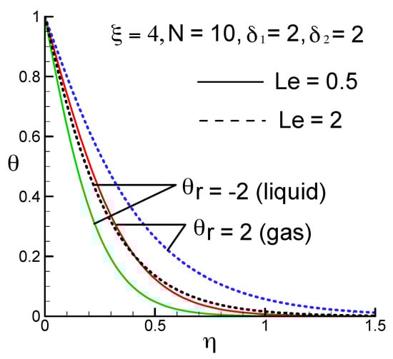
Figure 2.
The dimensionless temperature profile for two values of Le and .
In Figure 2, for = −2 and Le = 0.5, it is observed that the dimensionless wall temperature gradient is large. However, in Figure 3, for = −2 and Le = 2, it was found that the dimensionless wall concentration gradient is large. From Equation (23), Le = α/D, we can find that the increase in the Le leads to an increase in the thermal boundary layer thickness and a decrease in the concentration boundary layer thickness .
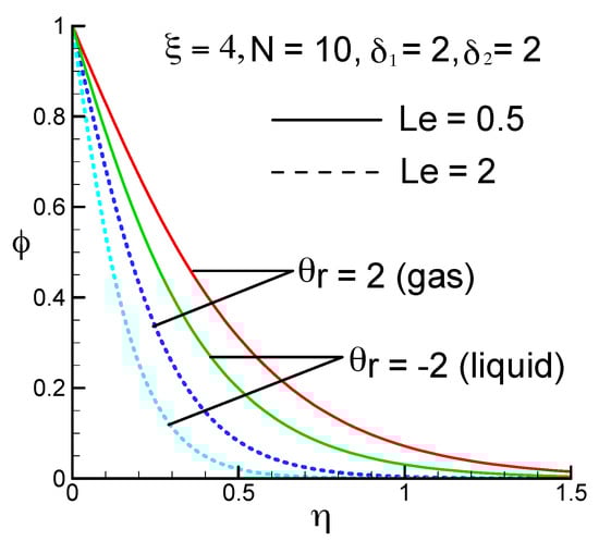
Figure 3.
The dimensionless concentration profile for two values of Le and .
Figure 4 and Figure 5 show the effects of the non-linear temperature parameter and the non-linear concentration parameter on the dimensionless temperature profile and the dimensionless concentration profile with ξ = 4, N = 10, Le = 0.5, = −2, respectively. In Figure 4 and Figure 5, for = 2 and = 2, it is observed that the dimensionless wall temperature gradient and the dimensionless wall concentration gradient are large. From Equation (16), as and become larger, the flow velocity becomes larger, and thus both the dimensionless wall temperature and concentration gradients increase.
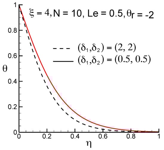
Figure 4.
The dimensionless temperature profile for two values of and .
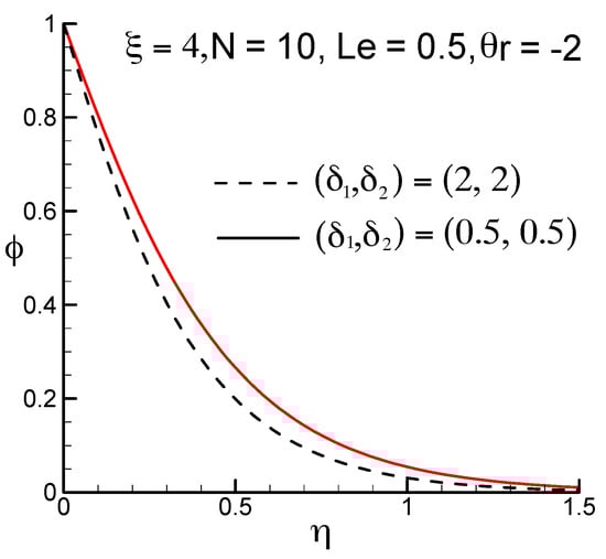
Figure 5.
The dimensionless concentration profile for two values of and .
The orthogonal table values of the local Nusselt number, the local Sherwood number, the local Nusselt number signal/noise ratio and the local Sherwood number signal/noise ratio are shown in Table 4. Using the values of the orthogonal table and the Taguchi analysis, we can obtain the Nusselt (Sherwood) number signal/noise ratio and mean value, as illustrated in Table 5 (Table 6). From the local Nusselt number and the signal/noise ratio, data can be obtained from the A factor is the level 3, B factor is the level 3, C factor is the level 1, D factor is the level 1, E factor is the level 2 or 3, and F factor is the level 3. From the local Sherwood number and the signal/noise ratio, data can be obtained from the A factor is the level 3, B factor is the level 3, C factor is the level 3, D factor is the level 1, E factor is the level 3, and the F factor is the level 3.
Table 4.
The orthogonal table values of the local Nusselt number, the local Sherwood number, the local Nusselt number signal/noise ratio and the local Sherwood number signal/noise ratio.
Table 5.
The results of the local Nusselt number and signal/noise ratio orthogonal table simulation.
Table 6.
The results of the local Sherwood number and signal/noise ratio orthogonal table simulation.
The results obtained using the Taguchi method are superior to the original combination of parameter settings. Using ξ (4), N (10), Le (0.5), (−2), (1 or 2), (2) in comparison with the highest value in the orthogonal table ξ (4), N (10), Le (0.5), (−2), (1), (1), the results show for the case of ξ (4), N (10), Le (0.5), (−2), (1), (2) and ξ (4), N (10), Le (0.5), (−2), (2), (2), that the local Nusselt numbers are 3.8318 and 3.8636, respectively. For ξ (4), N (10), Le (0.5), (−2), (1), (1), the local Nusselt number is 3.4053. Using ξ (4), N (10), Le (2), (−2), (2), (2) in comparison with the highest value in the orthogonal table ξ (4), N (10), Le (2), (2), (2), (2), the results show that the local Sherwood number is 5.1156 for the case of ξ (4), N (10), Le (2), (−2), (2), (2). For ξ (4), N (10), Le (2), (2), (2), (2), the local Sherwood number is 3.2799. It is known from the above verification by the Taguchi method that, for the cases of ξ (4), N (10), Le (0.5), (−2), (2), (2) and ξ (4), N (10), Le (2), (−2), (2), (2), the best data are obtained.
Table 7 lists the values of the local Nusselt number and the local Sherwood number for various values of , Le, , , N, ξ. As the increases from −2 to 2, the local Nusselt number and the local Sherwood number decrease. This is because for the case of > 0 (gas), both the dimensionless surface temperature and concentration gradients decrease, as shown in Figure 2 and Figure 3. As the Lewis number Le increases from 0.5 to 2, the local Nusselt number decreases. This is due to the fact that a larger Lewis number Le is associated with a thicker thermal boundary layer thickness, as shown in Figure 2. The thicker the thermal boundary layer thickness, the smaller the local Nusselt number. However, the concentration boundary layer thickness becomes thin, as shown in Figure 3. The thinner the concentration boundary layer thickness, the greater the local Sherwood number. With an increase in the non-linear temperature parameter and the non-linear concentration parameter from 0.5 to 2, the local Nusselt number and the local Sherwood number increase. That is because when increasing the non-linear temperature and concentration parameters, both the dimensionless wall temperature and concentration gradients increase, as shown in Figure 4 and Figure 5. With the help of Equations (26) to (27), the greater the dimensionless wall temperature (concentration) gradient, the greater the local Nusselt (Sherwood) number. Generally speaking, both the local Nusselt number and the local Sherwood number increase when the buoyancy ratio N increases from 1 to 10. This is due to the fact that the increase in the value of N tends to increase the buoyancy force, accelerating the flow and thereby the thermal boundary layer thickness and concentration boundary layer thickness become thin. Increasing the value of the dimensionless streamwise coordinate ξ enhances the local Nusselt number as well as the local Sherwood number. This is because the increase in the value of ξ decreases both the thermal boundary layer thickness and the concentration boundary layer thickness.
Table 7.
Values of the local Nusselt number and the local Sherwood number for , Le, , , N, ξ.
4. Conclusions
The conclusion of the first phase is as follows:
- As the viscosity-variation parameter increases from −2 (liquid) to 2 (gas), both the local Nusselt number and the local Sherwood number decrease.
- Increasing the Lewis number from 0.5 to 2 decreases the local Nusselt number, but increases the local Sherwood number.
- The local Nusselt number and the local Sherwood number increase with the increase in the non-linear temperature parameter and the non-linear concentration parameter .
- When the buoyancy ratio N increases from 1 to 10, the local Nusselt number and the local Sherwood number are increased.
- As the dimensionless streamwise coordinate ξ increases from 0 to 4, the local Nusselt number and the local Sherwood number increase.
The second phase is to invoke the Taguchi experimental method to replace the traditional single-factor experimental method. All parameter optimization design aims to find the maximum local Nusselt number and the local Sherwood number. The larger the local Nusselt number and local Sherwood number, the greater the amount of heat and mass will be that are taken away from the truncated cone. The number of experiments can be greatly reduced, effectively saving the computer simulation time. Computer numerical simulation shows that the maximum values of the local Nusselt number is 3.8636 for the case of ξ (4), N (10), Le (0.5), (−2), (2), (2), and the local Sherwood number is 5.1156 for the case of ξ (4), N (10), Le (2), (−2), (2), (2). It is very easy for engineers to use the numerical solution presented in this article to obtain the local values of heat and mass transfer characteristics.
Author Contributions
K.M.T., K.A.Y., F.I.C. and J.H.C. contributed in the paper equally. All authors have read and agreed to the published version of the manuscript.
Funding
This research was funded in part by the Ministry of Science and Technology, Taiwan, R.O.C., grant numbers MOST107-2221-E-992-086-MY3.
Conflicts of Interest
No conflict of interest.
Nomenclature
| a | constant |
| C | concentration |
| D | mass diffusivity |
| f | dimensionless stream function |
| g | gravitational acceleration |
| K | permeability of the porous medium |
| Le | Lewis number |
| N | buoyancy ratio |
| local Nusselt number | |
| p | pressure |
| local Rayleigh number | |
| r | local radius of the vertical truncated cone |
| local Sherwood number | |
| T | temperature |
| u | Darcy velocity in the x-direction |
| v | Darcy velocity in the y-direction |
| x | streamwise coordinate |
| distance measured from the leading edge of the vertical truncated cone | |
| distance of the leading edge of vertical truncated cone measured from the origin | |
| y | transverse coordinate |
| Greek symbols | |
| α | equivalent thermal diffusivity |
| coefficient of concentration expansion | |
| coefficient of concentration expansion | |
| coefficient of thermal expansion | |
| coefficient of thermal expansion | |
| γ | viscosity-variation constant |
| δ | half angle of the truncated cone |
| the non-linear temperature parameter | |
| the non-linear concentration parameter | |
| concentration boundary layer thickness | |
| thermal boundary layer thickness | |
| η | pseudo-similarity variable |
| θ | dimensionless temperature |
| viscosity-variation parameter | |
| μ | variable viscosity |
| ξ | dimensionless streamwise coordinate |
| density | |
| dimensionless concentration | |
| ѱ | stream function |
| Subscripts | |
| w | condition at the wall |
| ∞ | ambient |
Appendix A
Continuity Equation:
Momentum (Darcy) Equation:
Energy Equation:
Concentration Equation:
Non-Boussinesq approximation:
Boundary conditions:
Dimensionless non-similarity variables:
From Equations (A2) and (A3), if we do the cross-differentiation :
∵ Boundary layer approximation:
∴
From Equation (A5):
Then
Inserting Equation (A8b) into Equation (A8a), we obtain
Integrating Equation (A8c) once and via Equations and .
From Equation (A7) ,
From Equation (A7)
From (A1), we have ,
Substituting Equation (A7) into Equation (A9), with the help of , we obtain
Thus,
From Equation (A3)
Substituting Equation (A11a) to Equation (A11e) into Equation (A3), we obtain
Then
From Equation (A4)
Putting Equations (A11a)–(A11b) and Equation (A12a) to Equation (A12c) into Equation (A4), we get
Therefore
Then
Appendix B
The Keller-box method involves four key steps, which are described below:
- (B.1)
- Reducing the 5th-order partial differential equation system to five first order equations.
- (B.2)
- Writing the finite difference equations by using the central differences.
- (B.3)
- Linearizing the resulting algebraic equations with Newton’s method.
- (B.4)
- Expressing them in matrix–vector form and utilizing the block-tridiagonal elimination to solve the linear system.
References
- Cheng, P.; Le, T.T.; Pop, I. Natural Convection of a Darcian Fluid about a Cone. Int. Commun. Heat Mass Transf. 1985, 12, 705–717. [Google Scholar] [CrossRef]
- Yih, K.A. Coupled Heat and Mass Transfer by Free Convection over a Truncated Cone in Porous Media: VWT/VWC or VHF/VMF. Acta Mech. 1999, 137, 83–97. [Google Scholar] [CrossRef]
- Cheng, C.Y. An Integral Approach for Heat and Mass Transfer by Natural Convection from Truncated Cones in Porous Media with Variable Wall Temperature and Concentration. Int. Commun. Heat Mass Transf. 2000, 27, 537–548. [Google Scholar] [CrossRef]
- Cheng, C.Y. Soret and Dufour Effects on Heat and Mass Transfer by Natural Convection from a Vertical Truncated Cone in a Fluid-Saturated Porous Medium with Variable Wall Temperature and Concentration. Int. Commun. Heat Mass Transf. 2010, 37, 1031–1035. [Google Scholar] [CrossRef]
- Postelnicu, A. Free Convection from a Truncated Cone Subject to Constant Wall Heat Flux in a Micropolar Fluid. Meccanica 2012, 47, 1349–1357. [Google Scholar] [CrossRef]
- Chamkha, A.J.; EL-Kabeir, S.M.M.; Rashad, A.M. Coupled Heat and Mass Transfer by MHD Natural Convection of Micropolar Fluid about a Truncated Cone in the Presence of Radiation and Chemical Reaction. J. Nav. Archit. Mar. Eng. 2013, 10, 157–168. [Google Scholar] [CrossRef]
- Yih, K.A.; Huang, C.J. Effect of Internal Heat Generation on Free Convection Flow of Non-Newtonian Fluids over a Vertical Truncated Cone in Porous Media: VWT/VWC. J. Air Force Archit. Technol. 2015, 14, 1–18. [Google Scholar]
- Cheng, C.Y. Free Convection of a Nanofluid about a Vertical Truncated Cone. J. Chin. Soc. Mech. Eng. 2016, 37, 213–219. [Google Scholar]
- Amanulla, C.H.; Nagendra, N.; Suryanarayana Reddy, M. Thermal and Momentum Slip Effects on Hydromagnetic Convection Flow of a Williamson Fluid past a Vertical Truncated Cone. Front. Heat Mass Transf. 2017, 9, 1–9. [Google Scholar] [CrossRef]
- Mahdy, A. Modeling of Gyrotactic Microorganisms Non-Newtonian Nanofluids due to Free Convection Flow past a Vertical Porous Truncated Cone. J. Nanofluid 2018, 7, 603–612. [Google Scholar] [CrossRef]
- Lai, F.C.; Kulacki, F.A. The Effect of Variable Viscosity on Convective Heat Transfer along a Vertical Surface in a Saturated Porous Medium. Int. J. Heat Mass Transf. 1990, 33, 1028–1031. [Google Scholar] [CrossRef]
- Mahdy, A.; Chamkha, A.J.; Baba, Y. Double-Diffusive Convection with Variable Viscosity from a Vertical Truncated Cone in Porous Media in The Presence of Magnetic Field and Radiation Effects. Comput. Math. Appl. 2010, 59, 3867–3878. [Google Scholar] [CrossRef][Green Version]
- Mahdy, A. Effect of Chemical Reaction and Heat Generation or Absorption on Double-Diffusive Convection from a Vertical Truncated Cone in Porous Media with Variable Viscosity. Int. Commun. Heat Mass Transf. 2010, 37, 548–554. [Google Scholar] [CrossRef]
- Vajravelu, K.; Canon, J.R.; Leto, J.; Semmoum, R.; Nathan, S.; Draper, M.; Hammock, D. Non-Linear Convection at Porous Flat Plate with Application to Heat Transfer from a Dike. J. Math. Anal. Appl. 2003, 277, 609–623. [Google Scholar] [CrossRef]
- Prasad, K.V.; Vajravelu, K.; Gorder, R.A. Non-Darcian Flow and Heat Transfer along a Permeable Vertical Surface with Nonlinear Density Temperature Variation. Acta Mech. 2011, 220, 139–154. [Google Scholar] [CrossRef]
- Kameswaran, P.K.; Sibanda, P.; Partha, M.K.; Murthy, P.V.S.N. Thermophoretic and Nonlinear Convection in Non-Darcy Porous Medium. J. Heat Transf. 2014, 136, 042601. [Google Scholar] [CrossRef]
- Kameswaran, P.K.; Vasu, B.; Murthy, P.V.S.N.; Gorla, R.S.R. Mixed Convection from a Wavy Surface Embedded in a Thermally Stratified Nanofluid Saturated Porous Medium with Non-Linear Boussinesq Approximation. Int. Commun. Heat Mass Transf. 2016, 77, 78–86. [Google Scholar] [CrossRef]
- Ho, W.H.; Tsai, J.T.; Lin, B.T.; Chou, J.H. Adaptive Network-Based Fuzzy Inference System for Prediction of Surface Roughness in End Milling Process Using Hybrid Taguchi-Genetic Learning Algorithm. Expert Syst. Appl. 2009, 36, 3216–3222. [Google Scholar] [CrossRef]
- Chou, J.H. Optimization Methodology Course Handout; Department of Electrical Engineering, National Kaohsiung University of Applied Sciences: Kaohsiung, Taiwan, 2012. [Google Scholar]
- Kishore, R.A.; Kumar, P.; Sanghadasa, M.; Priya, S. Taguchi Optimization of Bismuth-Telluride Based Thermoelectric Cooler. J. Appl. Phys. 2017, 122, 025109-1–025109-12. [Google Scholar] [CrossRef]
- Li, Y.H.; Kao, W.C. Taguchi Optimization of Solar Thermal and Heat Pump Combisystems under Five Distinct Climatic Conditions. Appl. Therm. Eng. 2018, 133, 283–297. [Google Scholar] [CrossRef]
- Cebeci, T.; Bradshaw, P. Physical and Computational Aspects of Convective Heat Transfer; Springer: New York, NY, USA, 1984. [Google Scholar]
- Vajravelu, K.; Prasad, K.V.; Gorder, R.A.V.; Lee, J. Free Convection Boundary Layer flow past a Vertical Surface in a Porous Medium with Temperature-Dependent Properties. Trans. Porous Med. 2011, 90, 977–992. [Google Scholar] [CrossRef]
- Weast, R.C. CRC Handbook of Chemistry and Physics; CRC Press: Boca Raton, FL, USA, 1990. [Google Scholar]


© 2020 by the authors. Licensee MDPI, Basel, Switzerland. This article is an open access article distributed under the terms and conditions of the Creative Commons Attribution (CC BY) license (http://creativecommons.org/licenses/by/4.0/).