Abstract
With the recent rapid increase in the use of roof top photovoltaic solar systems worldwide, and also, more recently, the dramatic escalation in building grid connected solar farms, especially in Australia, the need for more accurate methods of very short-term forecasting has become a focus of research. The International Energy Agency Tasks 46 and 16 have brought together groups of experts to further this research. In Australia, the Australian Renewable Energy Agency is funding consortia to improve the five minute forecasting of solar farm output, as this is the time scale of the electricity market. The first step in forecasting of either solar radiation or output from solar farms requires the representation of the inherent seasonality. One can characterise the seasonality in climate variables by using either a multiplicative or additive modelling approach. The multiplicative approach with respect to solar radiation can be done by calculating the clearness index, or alternatively estimating the clear sky index. The clearness index is defined as the division of the global solar radiation by the extraterrestrial radiation, a quantity determined only via astronomical formulae. To form the clear sky index one divides the global radiation by a clear sky model. For additive de-seasoning, one subtracts some form of a mean function from the solar radiation. That function could be simply the long term average at the time steps involved, or more formally the addition of terms involving a basis of the function space. An appropriate way to perform this operation is by using a Fourier series set of basis functions. This article will show that for various reasons the additive approach is superior. Also, the differences between the representation for solar energy versus solar farm output will be demonstrated. Finally, there is a short description of the subsequent steps in short-term forecasting.
1. Introduction
This study is an extension of a paper presented at the 21st International Congress on Modelling and Simulation, Gold Coast, Australia [1]. Further justification of the argument for selecting the additive model for representing the seasonality of solar radiation has been added. Additionally, the discussion has been extended to include the differences for dealing with the seasonality of solar farm output as compared to solar radiation per se.
The literature includes a wide range of methods for forecasting solar radiation on different time scales. Two papers in particular [2,3] contain comprehensive reviews of recent articles in this area. The approaches range from use of Artificial Neural Networks (ANN) using solar irradiation, rather than some transformed variable [4], to several methods where the first step is some type of seasonal adjustment. This can take the form of multiplicative de-seasoning such as using clearness index or a clear sky model, or additive de-seasoning using Fourier series or wavelets. Before looking at these various methods of seasonal adjustment, let us examine the range of forecasting tools apart from that process of the modelling. Forecasting tools cover a broad range from ANN ([4,5,6] and several other references) to Adaptive Autoregressive [7] to Exponential Smoothing [8]. Several studies make use of what might be called hybrid models, like wavelets plus ANN [9,10,11], and the Coupled Autoregressive and Dynamical Systems (CARDS) model of the present author and colleagues [12]. This gives a flavour of the wide range of possible methods used for short-term forecasting of solar radiation. These all involve some form of mathematical or statistical approach, but there are also ways of utilising sky cameras, cloud motion vectors, satellite imaging, and so forth.
Seasonality
The methods above, regarding dealing with the inherent seasonality in sub-daily solar radiation series, have to be examined in detail, as characterising the seasonality is the first step in forecasting on hourly and sub-hourly time scales. As mentioned, one approach has been to use multiplicative de-seasoning in the form of dividing the solar radiation series by, in some cases, the extraterrestrial radiation over the site in question for the same time to produce the clearness index [13,14,15,16]. Alternatively, numerous articles deal with dividing the solar radiation by some clear sky model to create a clear sky index [5,7].
It is useful to examine whether a multiplicative model is used for describing the seasonality of solar radiation by necessity or for some historical reason. The most usual application of the multiplicative model is for economic series. This is because most seasonal economic series display seasonal variation that increases with the level of the series. For example, in time series that describe tourist arrivals [17], there are more arrivals in particular seasons, but also there can be more variability in those seasons as well. Often practitioners model the seasonality by first taking logarithms of the data in order to stabilise the variance. This approach has been also done with solar data by at least one researcher [18]. This method of using a logarithmic transform coupled with multiplicative de-seasoning for solar data might be a possible method since there is more pronounced variability in the summer months when there is a higher level in the series as well. It will be shown below that using an additive Fourier series representation of the seasonality is a very effective way of dealing with this phenomenon. Apart from this, one could make a case for the use of the clearness index rather than a clear sky model for multiplicative de-seasoning, even though [19] discussed the use of both methods and decided to use the clear sky index. One reason is that Ineichen [20] feels it is necessary to examine the relative efficacy of numerous clear sky models, whereas the clearness index has a well defined formulation. Inman et al. [2] present a poignant discussion on the viability of using clearness index versus clear sky index. The clear sky model requires input of local values of atmospheric variables such as ozone content, water vapour and turbidity. Alternatively, the extraterrestrial radiation only requires inputs such as latitude, time of year, and such like. It does not require data to be measured and input, and thus is not subject to atmospheric fluctuations.
There are many reasons why an additive model to describe the seasonality is more appropriate than a multiplicative one. In particular, a Fourier series approach displays a number of benefits. At any time throughout the year, the Fourier series representation gives the expected value of the variable in question. One could describe this as representing the climate for the location. The difference between the Fourier series model and the data at a particular time can be thought of as the influence of the weather. This could be for solar radiation as is being discussed here, or alternatively ambient temperature, electricity load, or other variables displaying similar seasonal characteristics. This is one of the valuable attributes referred to by Skeiker [21] when he talks of the physical meaning inherent in this representation, which other methods do not necessarily display. Some other researchers, for example, Dong et al. [8], discuss the important sub-diurnal cycles in solar radiation time series, but do not explain their presence from a physical point of view. As will be seen in later sections, the Fourier series approach lends itself very well to an exploration of the physical nature of these cycles. From a statistical viewpoint, simple formulae allow one to calculate the amount of variance of the original data explained by the Fourier series representation for each of the frequencies involved. Arguing against the use of the Fourier series approach, the comments put forward in [2] with respect to clear sky models might also apply here in that for estimating the Fourier coefficients one needs data for some particular period, some years for daily or hourly data down to some months for minute data. However, if ground station data is not available, there is data available that is inferred from satellite images. One could argue that there is no data from satellite models for the minute time scale, but the inherent smoothing provided by the Fourier model at a half hour time scale for instance infers values at lower time scales.
2. Fourier Series Representation
The present author [22] described the physical nature of the significant frequencies that are inherent in the solar radiation data. The yearly and daily cycles are intuitively obvious. The necessity of including the twice daily cycle, also identified by [8] is less obvious. It could represent the fact that as well as night being different from day, morning is different from afternoon. The question arises as to why one must include the frequencies just surrounding those two, at 364,365 and 729,731 cycles per year, the so-called sidebands or beat frequencies—see the power spectrum in Figure 1, where spikes are evident at those frequencies. This example is for the town of Mildura, Australia, latitude −34.22 for the year 2004.
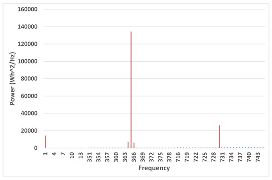
Figure 1.
Power spectrum for hourly solar radiation for Mildura data.
The concept of beat frequencies, also called sidebands, is well known in signal processing. In the language of that discipline, you can have a carrier signal with frequency that has its amplitude modulated by a signal at lower frequency . The manifestation of this change in amplitude resides in signals at frequencies , or in this case and for the daily cycle and a corresponding set of frequencies for the twice daily. T is the period, so for hourly data as an example.
Therefore, the Fourier series contains seven significant frequencies:
The first article discussing the use of Fourier series, including the beat frequencies, as a means of identifying the seasonality of solar radiation data, was [23]. In it, Phillips argued that with the use of 75 Fourier coefficients, a 20 year data set of a climatic variable could be represented without significant loss of information. He used solar radiation as his test data, but gave an interesting example of an extension. He discussed the solution of a differential equation involving a mass of lumped thermal capacitance, exposed to a solar flux and losing heat to ambient temperature. If the Fourier transforms of the solar flux and ambient temperature have been calculated, the differential equation in the time domain is transformed to an algebraic equation in the frequency domain, affording a much easier approach to solution. This same approach was taken by the present author [24] to construct the analytic solution to the differential equations governing heat flows in domestic dwellings.
One of the reasons why one might choose the multiplicative modelling of solar radiation is the change of amplitude with level of the series. With solar radiation series and other climate data series, the amplitude of the daily cycle changes as one progresses through the year. The amplitude is higher in summer than winter, progressing systematically, rather than probabilistically, throughout the year. The Fourier series representation, by including the beat frequencies, captures this systematic amplitude modulation. It is a transparent and formal method of representing this modulation.
See Figure 2 and Figure 3 for the effect of ignoring the sidebands. The model includes significantly non-zero values of solar radiation at night. Note that in these and subsequent figures, the term Data refers to the measured solar radiation values, and the term Model refers to the Fourier series representation of the data. Figure 4 illustrates the need for including the amplitude modulating frequencies. The data shown are the average daily values of solar radiation over the year, whereas the model is the Fourier series representation without the inclusion of the sidebands, averaged over the day. The values in the model at night have been zeroed as should be the case. This results in the bias shown with values too low in summer and too high in winter. Figure 5 depicts the same data as Figure 4, but the model now includes the sidebands frequencies. The addition of the sidebands means the model now follows the variation of the daily average in a more consistent manner over the year. It is internally consistent in that the physical interpretation of each term that is included is inherently simple and demonstrable. Figure 6 shows the performance of the Fourier series model with the sidebands included.
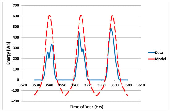
Figure 2.
Effect of no sidebands on winter solar radiation.
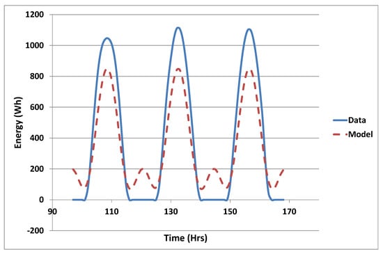
Figure 3.
Effect of no sidebands on summer solar radiation.
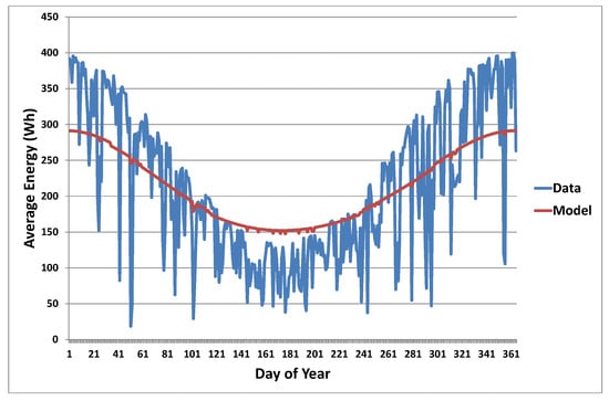
Figure 4.
Daily Average Solar Radiation data plus model with no sidebands.
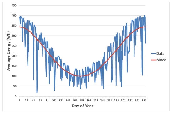
Figure 5.
Daily Average Solar Radiation data plus model with sidebands included.
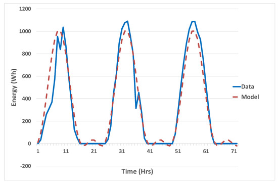
Figure 6.
Effect of including sidebands on solar radiation.
3. Fourier Series Model for a Tropical Location
There is an interesting contrast in the analysis for a tropical location, the island of Desirade, part of Guadeloupe in the French West Indies, latitude 16.32. Inspection of the power spectrum in Figure 7 hints at the fact that there may not be a significant change in the daily amplitude over the year. There are no apparent sidebands present in this graph. So, is this borne out? Let us examine a comparison of the data for a few days in summer plus a Fourier series model with sidebands and also one without the contribution from the sideband frequencies—Figure 8. There is very little difference with or without the contribution at the sideband frequencies. The difference between Desirade and Mildura can also be seen in Figure 9 for the daily mean solar radiation over the year for Desirade as compared with Figure 5 that shows the variation in daily amplitude over the year for Mildura.
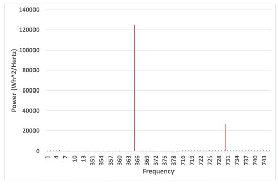
Figure 7.
Power spectrum for Desirade.
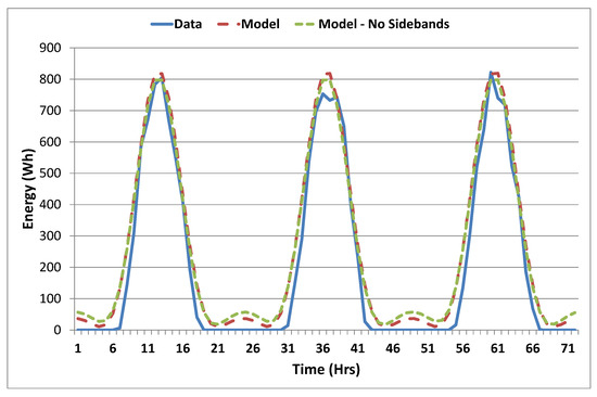
Figure 8.
Comparison of Fourier series model with and without sidebands—summer in Desirade.
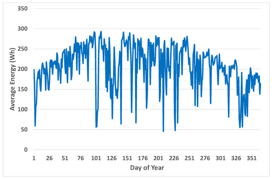
Figure 9.
Daily mean solar radiation for Desirade.
An additional analysis was done for a location whose latitude is between Mildura and Desirade. St Pierre, Reunion Island, is at latitude −21.34. An examination of the comparison of using the contribution from the sideband frequencies versus removing that contribution is given in Figure 10. It is obvious that the contribution at the sideband frequencies is more significant than at the tropical location, but less so than at the mid-latitude location, exactly as one might surmise. The decrease in importance of the sidebands for describing the seasonality as one traverses from mid-latitude in Mildura to lower latitude in St. Pierre, and even lower in Desirade, is due to the corresponding decrease in change of amplitude of the daily cycle over the year. As one draws closer to the equator, the daily amplitude approaches a constant. Interestingly, we will see a similar pattern with the output from solar farms in Australia in a subsequent section. Note that this type of information is not evident from using clear sky model multiplicative de-seasoning. Other limitations of the clear sky index approach will be given below.
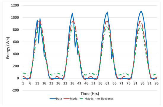
Figure 10.
Comparison of Fourier series model with and without sidebands—summer in St Pierre.
4. Correspondence with Other Seasonal Climate Variables
There are situations where bivariate models of climate variables are necessary. If one of the components is solar radiation, then an alternative to the use of a clear sky model must be used, as there is no equivalent formulation for other climate variables. Examples have been given in [23,24]. Skeiker [21] illustrates that it represents the temperature seasonality very well. Even though there are situations where one does not have to treat all variables with the same methods, there is a good example of the need to do so with solar radiation and temperature. To model the performance of crystalline solar cells, it is necessary to build a bivariate model for the two variables. Ambient temperature has a lagged dependence on solar radiation, and as the efficiency of the solar cells is dependent on temperature as well as the incoming solar radiation, the two variables must be modelled in tandem. There is no temperature equivalent of a clear sky model, so an efficient method of modelling the seasonality of the two variables in a corresponding manner is through using Fourier series.
5. Clear Sky Models
The clear sky index (CSI) is defined as the solar irradiance divided by a suitable clear sky model. As stated previously, there are numerous clear sky models [20].
One expects the clear sky index to be bounded in the interval . Because of the phenomenon of cloud enhancement (see [25]), it is possible to have some values greater than one. However, when we examine the CSI values for Las Vegas hourly data for 2010, constructed using the Bird clear sky model [26], we notice some problems. First, restrict the data to times for which the solar altitude , as there can be odd effects near sunrise and sunset. This stipulation is commonly used in evaluating forecasting for instance. Examining the histogram of values of CSI in Figure 11, the first problem is evident, as there are significant numbers of values greater than one. The second problem is visible in Figure 12, in that values at the beginning and end of each day for clear days are inflated. In essence one could say this is an induced seasonality, in that there is a U-shaped pattern from morning to afternoon.
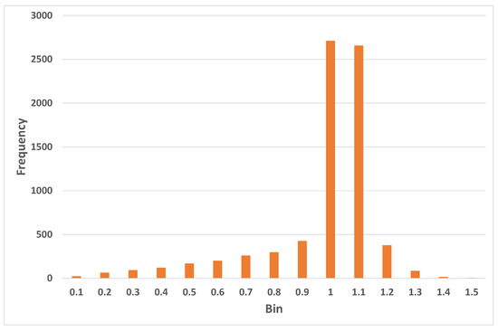
Figure 11.
Histogram of CSI values for Los Vegas.
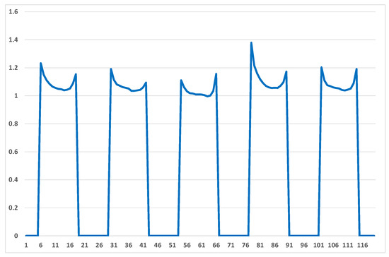
Figure 12.
Five days of CSI for Los Vegas.
6. Solar Farms, the Australian Perspective
As of June 2019, Australia had over 12,000 MW of installed PV, with 4000 MW being commissioned in the previous 12 months. The largest solar farm is 220 MW (Bungala in SA) and there are thirteen over 100 MW. The Australian Renewable Energy Agency (ARENA) has funded a number of consortia to improve the very short-term forecasting of solar farm output. The present author, in conjunction with researchers from the University of New South Wales (UNSW) and the Commonwealth Science and Industrial Research Organisation (CSIRO) were awarded a grant in July 2019 for $1.25 million over 18 months for the project entitled Solar Power Ensemble Forecaster. The partner solar farms in the project are at Manildra, Clare, Darling Downs, Gannawarra, Parkes, Hayman, in the eastern states of Australia.
In Australia, the National Electricity Market (NEM) is controlled by the Australian Energy Market Operator (AEMO), who are also in charge of maintaining the electricity grid for the area that the NEM covers, Queensland, New South Wales, Victoria, Tasmania and South Australia. Because of its remoteness, Western Australia maintains a separate system. The NEM is unique in its operation in the following ways.
- Every 5 min, scheduled generators supply a bid stack, with the amount of energy they can provide in the next 5 min at each of 10 price bands, from −$1000 to $14,000.
- AEMO then runs a linear program for each region of the NEM to determine how far up the bid stack they have to go to satisfy their forecasted net load.
- This determines the 5 min price for all energy, and the mean of 6 five minute prices gives the spot price for the half hour.
- Note. There are also semi-scheduled and non-scheduled generators. Neither bid, but semi-scheduled can be curtailed in there is already sufficient supply in the system.
One big problem for AEMO is that their forecast model, the Australian Solar Energy Forecast System (ASEFS), is relatively crude. To the best of my knowledge they use a form of persistence, . Interestingly, the next few figures will show that the output is capped and so on a clear day the output is close to constant for a number of hours.
We begin by comparing the profile of solar radiation over the day in Figure 13 with that of solar farm output for both summer in Figure 14 and winter in Figure 15. For the radiation, it is for a clear day but for the output it can be for partially cloudy days as well. Obviously for the solar radiation on a clear day, there is a definite peak in the profile around solar noon, whereas for the farm output in both seasons, there is a definite cap. It is conjectured that this is for a specific reason, as solar panels have become relatively cheap in recent years compared to value of the electrical equipment for transferring the energy to the grid. Thus, it is relatively inexpensive to oversize the field. If, for instance, one has a power purchase agreement (PPA) with a customer, if one oversizes the field, it is easier to be confident of supplying the contracted energy on the majority of days. That lessens the need for purchasing energy on the spot market to supply the contracted amount.
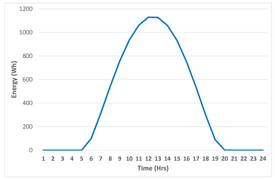
Figure 13.
Solar radiation profile.
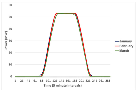
Figure 14.
Clear day solar farm output, January–March.
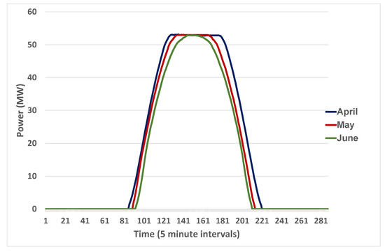
Figure 15.
Clear day solar farm output, April–June.
This results in an interesting change in the power spectrum of the farm compared with that of solar radiation—see Figure 16. There is virtually no yearly cycle to the embedded in the data, and related to this, there are essentially no beat frequencies. This is consistent with output reaching capacity on days in both winter and summer. The power spectrum is similar to that of solar radiation for a location close to the equator like Desirade discussed above.
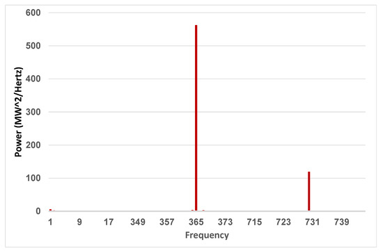
Figure 16.
Solar farm output power spectrum.
7. Forecasting the Non-Seasonal Residuals
Any additive one step ahead statistical forecasting method can be encapsulated by the structure
where is the solar radiation, is the difference between the solar radiation and the seasonality and denotes the representation of the seasonality. The denote possible exogenous variables. Knowledge of the statistical qualities of the errors, or noise terms, is necessary in order to construct the error bounds of the forecast. In this formulation, it is hoped, and sometimes assumed, that is independent and identically distributed (i.i.d.).
For solar data, the are uncorrelated but dependent. Note that correlation is only a linear property, so higher moments can be, and are, correlated. The are not identically distributed—they vary both systematically, with the variance higher in the summer than winter and in the middle of the day compared to morning and afternoon. They also can vary time step to time step in a conditional manner. However, in what follows, we are not interested in forming error bounds on that forecast, so that will be left to future work.
After the seasonality model has been identified the algorithm for forecasting the de-seasoned data is as follows.
- Form , where is either solar radiation or the solar farm power output in , and is the Fourier series representation of the climate.
- Check the sample autocorrelation function (SACF) and sample partial autocorrelation function (SPACF) to see what form of an should be used.
- There are two things to note here:
- -
- The Fourier series and models are estimated on a training set and then tested on a period of time not in the training set.
- -
- Many people at this stage use much more esoteric means for modelling, like ANN or other machine learning techniques.
Illustrative Results
In [12], the authors compare the use of Fourier series for seasonality and an autoregressive (AR) model (named CARDS) for forecasting the non-seasonal components with a number of models that combine clearness sky index and various ANN or ANN mixed with other tools. This is for forecasting solar radiation on an hourly time scale. The CARDS (coupled autoregressive and dynamical system) model performs at least as good as the other models. Since the forecasting of the non-seasonal component uses a basic low order AR model, the inference is that the Fourier series component is adept at handling the seasonality. Note that it was difficult to use exactly the same data as the researchers who developed the other models, but great care was taken to be as conservative as possible in setting up the experiments.
A more direct comparison was possible in [27], where the present author worked with colleagues from the Universit de La Reunion to compare forecasting for island versus continental sites. A secondary goal was to compare the performance at both types of sites of the use of Fourier series plus an AR model (FSAR), clear sky index plus ANN and clear sky index plus AR. All three versions performed similarly in terms of the standard error measures of bias, mean absolute error and root mean square error. The salient difference is that the FSAR model is inherently simpler—and would be deemed so quantitatively if one used the Akaike or Bayesian Information Criteria for comparison. The components of the model all display knowledge of the climate of the site under consideration.
Note how the use of the Fourier series approach and an autoregressive model for the residuals once the seasonality is removed performs in an operational mode for the solar farm output forecast. Operational mode means that the forecast has to be made for a five minute interval at least 70 s before the beginning of the interval. This is to allow the communication of the forecast to AEMO so the mechanisms for any necessary frequency control or additional generation can be enacted. Also, the forecast mechanism is recalibrated, for both the Fourier series and autoregressive components, every five minutes in a rolling window. This is done to cater for any changing conditions in the farm or in the climate in the region around the farm. Preliminary comparisons were performed for four solar farms. This approach was found to outperform the method used at present by AEMO by between 8% and 36% over the four farms.
8. Conclusions
There are three methods in the literature for describing the seasonality of solar radiation, and all have been discussed here to lesser or greater degree. The clearness index formulation has been used but is probably more in use in the development of statistical models for diffuse solar radiation—see, for example, in [28]. For forecasting of solar radiation, the majority of practitioners would use the clear sky index. The crux of this paper is an argument for selecting the Fourier series method for describing the seasonality. The reasons include the following.
- There are several clear sky models so how does one choose the one to use? It may be that different ones work better in some climates and others in different climates.
- For the clear sky model described in this paper, there were technical difficulties in its application to data from Los Vegas.
- The components of the Fourier series representation have a direct physical interpretation.
- The Fourier series representation is compatible with the representation of seasonality of other climate variables, like temperature, and even some variables that are at least somewhat dependent on climate like electricity demand.
And finally, there is another important consideration. One can imagine that there was a very important practical consideration for adopting the use of the clear sky index. In Australia, for example, there are very few locations for which there are high frequency measurements of the components of solar radiation over an extended period of time. As the construction of the discrete Fourier series representation is empirically based, it is best to have at hand a number of years of reasonable quality data with which to estimate the coefficients, particularly if one is interested in hourly forecasting tools for instance. If instead, one can make use of a physical clear sky model, and then apply it to whatever short series is of interest to obtain clear sky index values, that might seem to be appealing. However, perhaps this argument is now superseded, as even where there are no ground measurements, there exist long periods of gridded data derived from models that estimate global horizontal radiation from satellite images. These are typically available for the hourly time scale and increasingly for higher frequencies. One can build Fourier series models from these data. Thus, there are compelling reasons for the use of Fourier series to represent the seasonality of both solar radiation and solar farm output.
Funding
This research was funded by the Australian Renewable Energy Agency (ARENA) grant for Solar Power Ensemble Forecaster—$1.25 million over 18 months. Chief investigators are Boland (UniSA), Kay (UNSW), Huang, West, Knight (CSIRO). The partner solar farms are Manildra, Clare, Darling Downs, Gannawarra, Parkes, Hayman.
Conflicts of Interest
The author declares no conflict of interest.
Abbreviations
The following abbreviations are used in this manuscript:
| MDPI | Multidisciplinary Digital Publishing Institute |
| DOAJ | Directory of open access journals |
| TLA | Three letter acronym |
| LD | linear dichroism |
| AEMO | Australian Energy Market Operator |
| ARENA | Australian Renewable Energy Agency |
| UNSW | University of New South Wales |
| PPA | Power purchase agreement |
References
- Boland, J. Additive versus Multiplicative Seasonality in Solar Radiation Time Series. In Proceedings of the 21st International Congress on Modelling and Simulation, Modelling and Simulation Society of Australia and New Zealand, Gold Coast, Australia, 29 November–4 December 2015; pp. 1126–1132. [Google Scholar]
- Inman, R.; Pedro, H.C.; Coimbra, C.M. Solar forecasting methods for renewable energy integration. Prog. Energy Combust. Sci. 2013, 39, 535–576. [Google Scholar] [CrossRef]
- Diagne, M.; David, M.; Lauret, P.; Boland, J.; Schmutz, N. Review of solar irradiance forecasting methods and a proposition for small-scale insular grids. Renew. Sustain. Energy Rev. 2013, 27, 65–76. [Google Scholar] [CrossRef]
- Sfetsos, A.; Coonick, A. Univariate and multivariate forecasting of hourly solar. Sol. Energy 2000, 68, 169–178. [Google Scholar] [CrossRef]
- Kemmoku, Y.; Orita, S.; Nakagawa, S.; Sakakibara, T. Daily insolation forecasting using a multi-stage neural network. Sol. Energy 1999, 66, 193–199. [Google Scholar] [CrossRef]
- González-Romera, E.; Jaramillo-Morán, M.A.; Carmona-Fernández, D. Monthly electric energy demand forecasting with neural networks and Fourier series. Energy Convers. Manag. 2008, 49, 3135–3142. [Google Scholar] [CrossRef]
- Bacher, P.; Madsen, H.; Nielsen, H.A. Online short-term solar power forecasting. Sol. Energy 2009, 83, 1772–1783. [Google Scholar] [CrossRef]
- Dong, Z.; Yang, D.; Reindl, T.; Walsh, W.M. Short-term solar irradiance forecasting using exponential smoothing state space model. Energy 2013, 55, 1104–1113. [Google Scholar] [CrossRef]
- Cao, J.C.; Cao, S.H. Study of forecasting solar irradiance using neural networks with preprocessing sample data by wavelet analysis. Energy 2006, 31, 3435–3445. [Google Scholar] [CrossRef]
- Cao, J.; Lin, X. Study of hourly and daily solar irradiation forecast using diagonal recurrent wavelet neural networks. Energy Convers. Manag. 2008, 49, 1396–1406. [Google Scholar] [CrossRef]
- Mellit, A.; Benghanem, M.; Kalogirou, S.A. An adaptive wavelet-network model for forecasting daily total solar-radiation. Appl. Energy 2006, 83, 705–722. [Google Scholar] [CrossRef]
- Huang, J.; Korolkiewicz, M.; Agrawal, M.; Boland, J. Forecasting solar radiation on an hourly time scale using a coupled autoregressive and dynamical system (CARDS) model. Sol. Energy 2013, 87, 136–149. [Google Scholar] [CrossRef]
- Martín, L.; Zarzalejo, L.F.; Polo, J.; Navarro, A.; Marchante, R.; Cony, M. Prediction of global solar irradiance based on time series analysis: Application to solar thermal power plants energy production planning. Sol. Energy 2010, 84, 1772–1781. [Google Scholar] [CrossRef]
- Aguiar, R.; Collares-Pereira, M. TAG: A time dependent, autoregressive, gaussian model for generating synthetic hourly radiation. Sol. Energy 1992, 49, 167–174. [Google Scholar] [CrossRef]
- Cena, V.; Mustacchi, C.; Rocchi, M. Stochastic simulation of hourly global radiation sequences. Energy 1979, 23, 47–51. [Google Scholar]
- Skartveit, A.; Olseth, J. The probability density and autocorrelation of short-term global and beam irradiance. Sol. Energy 1992, 49, 477–487. [Google Scholar] [CrossRef]
- Lim, C.; Mcaleer, M. Forecasting tourist arrivals. Ann. Tour. Res. 2001, 28, 965–977. [Google Scholar] [CrossRef]
- Reikard, G. Predicting solar radiation at high resolutions: A comparison of time series forecasts. Sol. Energy 2009, 83, 342–349. [Google Scholar] [CrossRef]
- Paoli, C.; Voyant, C.; Muselli, M.; Nivet, M. Forecasting of preprocessed daily solar radiation time series using neural networks. Sol. Energy 2010, 84, 2146–2160. [Google Scholar] [CrossRef]
- Ineichen, P. Comparison of eight clear sky broadband models against 16 independent data banks. Sol. Energy 2006, 80, 468–478. [Google Scholar] [CrossRef]
- Skeiker, K. Mathematical representation of a few chosen weather parameters of the capital zone Damascus in Syria. Renew. Energy 2006, 31, 1431–1453. [Google Scholar] [CrossRef]
- Boland, J. Time series and statistical modelling of solar radiation. In Recent Advances in Solar Radiation Modelling; Badescu, V., Ed.; Springer: Berlin/Heidelberg, Germany, 2008; Chapter 11; pp. 283–312. [Google Scholar]
- Ruppert, M.G.; Harcombe, D.M.; Ragazzon, M.R.P.; Moheimani, S.O.R.; Fleming, A.J. A review of demodulation techniques for amplitude-modulation atomic force microscopy. Beilstein J. Nanotechnol. 2017, 8, 1407–1426. [Google Scholar] [CrossRef] [PubMed]
- Boland, J. The Analytic Solution of the Differential Equations Describing Heat Flow in Houses. Build. Environ. 2002, 37, 1027–1035. [Google Scholar] [CrossRef]
- Starke, A.R.; Lemos, L.F.L.; Boland, J.; Cardemil, J.M.; Colle, S. Resolution of the Cloud Enhancement Problem for One-Minute Diffuse Radiation Prediction. Renew. Energy 2018, 125, 472–484. [Google Scholar] [CrossRef]
- Bird, R.E.; Hulstrom, R.L. A Simplified Clear Sky Model for Direct and Diffuse Insolation on Horizontal Surfaces; SERI–TR-642-761; Solar Energy Research Institute: Golden, CO, USA, 1981. [Google Scholar]
- Boland, J.; David, M.; Lauret, P. Short term solar radiation forecasting: Island versus continental sites. Energy 2016, 113, 186–192. [Google Scholar] [CrossRef]
- Ridley, B.; Boland, J.; Lauret, P. Modelling of diffuse solar fraction with multiple predictors. Renew. Energy 2010, 35, 478–483. [Google Scholar] [CrossRef]


© 2020 by the author. Licensee MDPI, Basel, Switzerland. This article is an open access article distributed under the terms and conditions of the Creative Commons Attribution (CC BY) license (http://creativecommons.org/licenses/by/4.0/).