Article

Evolution of Virtual Water Transfers in China’s Provincial Grids and Its Driving Analysis

Guangxi Key Laboratory of Power System Optimization and Energy Technology, Guangxi University, Nanning 530004, Guangxi, China
*
Author to whom correspondence should be addressed.
Energies 2020, 13(2), 328; https://doi.org/10.3390/en13020328
Submission received: 19 November 2019 / Revised: 10 December 2019 / Accepted: 16 December 2019 / Published: 9 January 2020
(This article belongs to the Special Issue Energy-Water Nexus)

Abstract

:
In China, electricity transmission has increased rapidly over the past decades, and a large amount of virtual water is delivered from power generation provinces to load hubs. Understanding the evolution of the virtual water network embodied in electricity transmission is vital for mitigating water scarcity. However, previous studies mainly calculated the virtual water transferred in short periods in low-spatial resolution and failed to reveal driving forces of the evolution of virtual water. To solve this problem, we investigated the historical evolution of the virtual water network and virtual scarce water network embodied in interprovincial electricity transmission between 2005 and 2014. The driving forces of the evolution of virtual (scarce) water networks were analyzed at both national level and provincial level. The results show that the overall virtual water transmission and virtual scarce water transmission increased by five times, and the direction was mainly from southwest and northwest provinces to eastern provinces. Sichuan, Yunnan, and Guizhou played an increasingly important role in virtual water exporting, and northwestern provinces had dominated the virtual scarce water exporting in the decade. At the national level, the increase of virtual water is mainly driven by the change of power generation mix and power transmission. At the provincial level, the increase of virtual water transmission in the largest virtual water exporter (Sichuan) is driven by the power generation mix and the power transmission, between 2005 and 2010, and 2010 and 2014, respectively. Considering the expanding of electricity transmission, the development of hydropower in the southwestern provinces and other renewable energies (solar and wind) in the northeastern provinces would overall mitigate the water scarcity in China.

1. Introduction

Water scarcity is serious in China, and per capita water resources are only 25% of the average world level [1]. The spatial and temporal distribution of water resources is extremely unbalanced [2]. Over 80% of water resources are reserved in southern China, while northern China sustains 47% of people with less than 20% of water resources. Water scarcity has become a major bottleneck restricting the sustainable development of the economy and society [3]. The Chinese government has implemented the strictest regulation to mitigate water scarcity, e.g., constraining the total use of water resources within 700 billion cubic meters by 2030 [4]. Industry sectors consumed 126 billion cubic meter water accounting for 20% of the total water consumption in 2018 [5]. Among all industrial sectors, the power system is the largest water consumer contributing to 70% of the total industrial water consumption [6]. Therefore, investigating electricity-related water consumption is a key aspect to mitigate water scarcity in China.
To investigate water stress posed by the power system, previous studies have quantified direct water use or consumption of power generation in China [7,8], focusing on different power generation technologies [9,10], environmental impacts [11,12] and future scenarios analysis [13,14]. To further quantify the life cycle water consumption of functional electricity (kWh), virtual water (VW) was introduced in the investigation for electricity-water nexus. The concepts of virtual water and water footprint were proposed to quantify water consumption through the life cycle of a commodity [15,16]. The life cycle water use of power generation was estimated through different methods [17,18] or at different spatial scales [19,20,21]. For instance, Feng et al. [17] used the hydro-life-cycle-analysis method to calculate water coefficients of eight power generation types, and they found the water coefficient of hydropower is higher than that of thermal power. Besides, electricity is transferred from arid western provinces to eastern provinces. The mismatch between energy resources and water resources in China has raised many concerns regarding potential water-related impacts from power transmission.
According to the virtual water strategy [16], VW flows are transferred from the source to the sink and thus reallocates the water resources on both sides. In the power system, VW is delivered from power generation provinces to load hubs through electricity transmission, which may induce water scarcity. Multiple studies have explored the virtual water network through electricity transmission in recent years. For instance, Zhu et al. [20] and Guo et al. [21] developed a node-flow model to calculate the virtual water transmission (VWT) among six sub-national grids in the year 2010 and short-time span (2007–2012), respectively. Zhang et al. [22] quantified the interprovincial VWT embodied in thermal power transmission and adjusted VW into virtual scarce water (VSW) in 2011, by improving the spatial resolution to the provincial level and combining the water stress index (WSI). The aforementioned studies proved that VWT extremely exacerbated the local water scarcity in power generation provinces, especially in northwestern provinces. In USA, Chini et al. [23] explored the blue water and grey water transfers embodied in power grids and provided clear grey water and blue water network. In addition, some studies identified whether the virtual water flows mitigate or exacerbate the water scarcity by comparing the WSI of source and sink [24]. However, there is a lack of study for the evolution of VWT embodied in electricity transmission.
Electricity transmission has increased by 4.2 times in the last decade [25], resulting in a significant increase of VWT. To explore the evolution of VWT, the decomposition analysis is introduced to reveal the driving forces of the evolution of the virtual water network. The decomposition analysis was proposed to quantify different contributions of factors to the change of an indicator between two periods. Structural decomposition analysis (SDA) and index decomposition analysis (IDA) are two widely used approaches to investigate electricity consumption related indicators, such as carbon emissions [26,27] and virtual water consumption [28,29]. Logarithmic Mean Divisia Index (LMDI) is the most popular IDA method with low-resolution data requirements and simplicity. It could also be used to investigate electricity-related carbon emission [30] and water consumption [31]. However, unlike SDA, LMDI cannot distinguish final demand and intermediate demand, thus, the indirect impacts of change in final demand cannot be estimated. To estimate the contribution of indirect impacts to the overall changes of energy-related indicators, the SDA method was widely used. Nevertheless, SDA is restricted by its high-quality data requirements based on the input-output (IO) table. Research [32] proposed a modified SDA based on the electricity transmission table to analyze the contribution of factors (especially for the change of power transmission) to the increase of carbon emission in the power sector. Electricity-related water footprint differs from carbon footprint because water resources vary from region to region when carbon emissions have the same effects on climate change regardless of location. Paper [33] investigated the driving forces for the evolution of VWT embodied in thermal power generation, and the results showed that water efficiency improvements were the main driver to the decrease of VWT at the national level. However, the analysis in paper [33] is not comprehensive, because only thermal power was considered, and the differences of driving forces in various provinces were not included. During the last decades, China’s power generation and transmission have expanded significantly, which was largely driven by renewable energy technologies. Hydropower has a higher water coefficient than thermal power because of evaporation in reservoir. A deep investigation of the evolution of virtual water transfers is necessary for the understanding of water-electricity nexus.
This study investigated the long-time series evolution of virtual (scarce) water network embodied in interprovincial electricity trade, and further identified the driving factors to the change of the virtual (scarce) water transmission by using a modified SDA model. Compared to previous studies, the novelty and significance of this work are as follows: (1) water consumption for all power generation technologies (including thermal, hydropower, wind, solar, and nuclear) are included; (2) VW network and VSW network are both investigated to represent the imbalance spatial distribution of water resources in different provinces; and (3) by using a modified SDA model, a high-resolution decomposition results are analyzed to capture the contribution of different factors at both national level and provincial level.
The structure of this study is into two parts. In part 1, Section 2.1 and Section 2.2 constructed the node-flow model of the virtual water network, and the SDA model for investigating the driving factors, respectively. Section 2.3 and Section 2.4 introduced the spatial and temporal area of the paper and the data sources. In part 2, Section 3 shows the results for the VW network evolution and its driving factors. Section 4.1 and Section 4.2 discussed the impacts of different policies between 2005 to 2014 and advice for Chinese policymaker, while Section 4.3 discussed the limitation and advantages in this study.

2. Materials and Methods

2.1. Modeling Virtual Water Network Embodied in Electricity Trade

Based on the node-flow model proposed in previous studies [20,21], we modelled inter-provincial electricity transmission as a network with nodes and flows. Each province and each electricity trade is assumed as a node and a flow, respectively. For each node, the total power demand is supplied by local power generation and power imported from other nodes; local plants can only outflow power to satisfy the local demand and other nodes. The transmission loss is ignored in this study, and the balance between power generation and power demand for each node can be expressed below:
i = m i = 1 E D i + i = m , i j i = 1 E T i j = i = m i = 1 E G i + j = m , j i j = 1 E T j i
where EGi is the electric power generation of node i, EDi is the power demand of node i, and ETij is the electricity flow from node i to node j.
The balance between power demand and power generation can be adapted to the virtual water transfers by Equation (2):
i = m i = 1 E G i · d w i + i = m , i j i = 1 E T i j · t w j = ( i = m i = 1 E D i + j = m , j i j = 1 E T j i ) · t w i
where dwi represents the direct water consumption factor for functional unit power generation in province i, and twj represents the embodied water footprint (total water consumption factor) of functional unit power supplied by province j.
We assume that all electricity feeding into province i is totally mixed, i.e., from different sources. The embodied water footprint of electricity supplied to local users is thus the same as the electricity exported to other nodes for provinces i. To calculate twi, Equation (2) can be rearranged into Equations (3) and (4):
i = m i = 1 E G i · d w i = ( i = m i = 1 E D i + j = m , j i j = 1 E T j i ) · t w i i = m , i j i = 1 E T i j · t w j
E ^ G · D W = M · T W
where E ^ G represents the diagonal matrix of electricity generation E G i , DW represents the column of d w i , TW represents the column of t w i , and M is rearranged as electricity trade matrix given by Equation (5):
M = [ j 1 E T 1 j + E d , 1 E T 21 E T m 1 E T 12 j 2 E T 2 j + E d , 2 E T m 2 E T 1 m E T 2 m j m E T 2 j + E d , 2 ]
The vector of total water coefficient can be calculated in the following:
T W = M 1 · E ^ D · D W = H · D W
By using Equation (6), we create a linear map between the direct water coefficient and the virtual water coefficient, thus link the water footprint from the electricity consumption side to the production side. Each element in matrix H, hij, represents the complete electricity transmission, which is different from the direct electricity transmission, because it includes higher-order electricity transmission. The role of H is the same as the role of Leonfief matrix in the input–output analysis which transforms the direct consumption to the total consumption.

2.2. Virtual Water Transmission and Decomposition Analysis Model
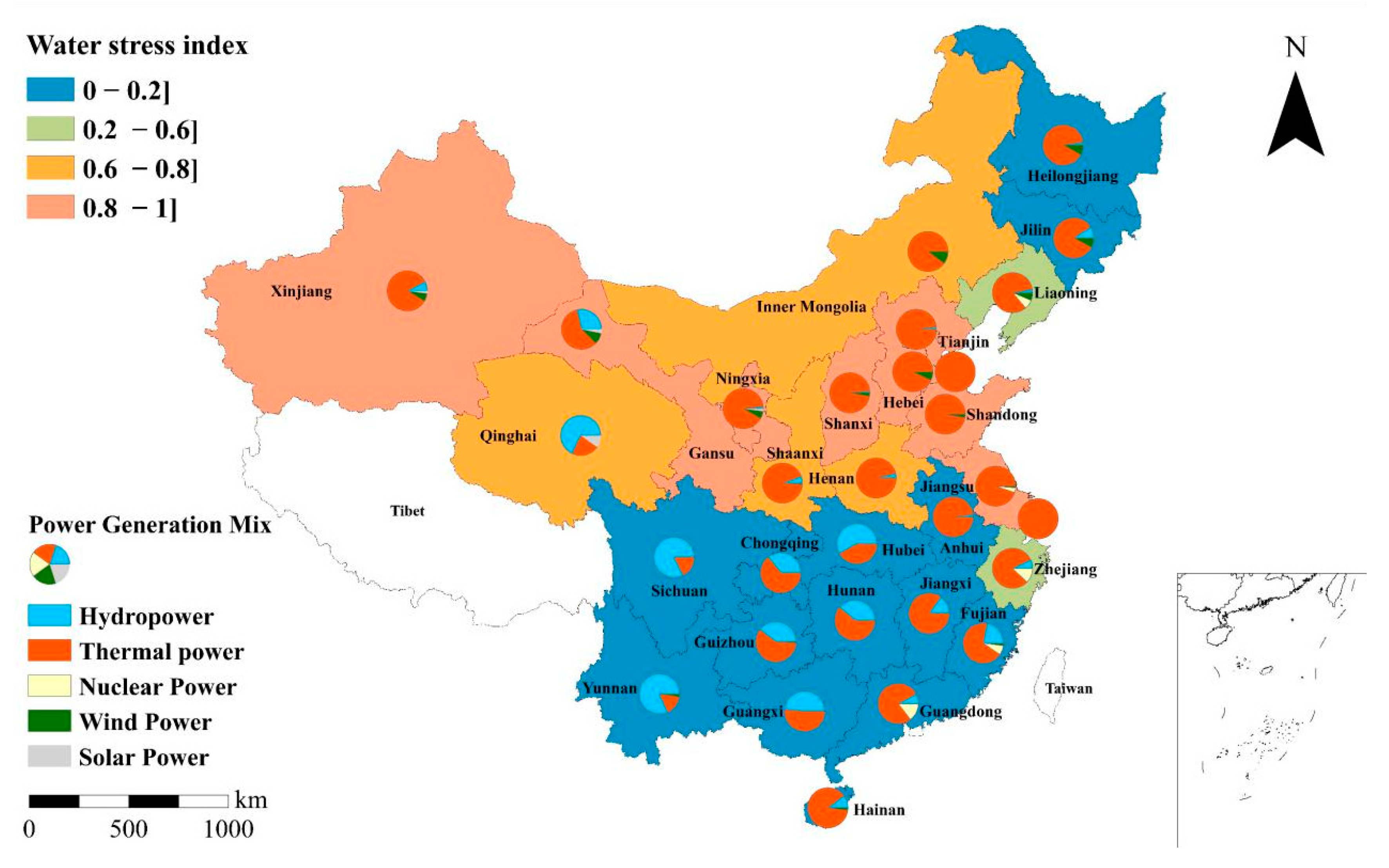
SDA can estimate the contribution of different factors to the overall evolution of an indicator, and it has been widely used to investigate the energy-related emissions. However, SDA is highly depended on the IO table, which restricts the application of itself. According to a previous study [32], a modified SDA model applying the electricity transmission table (not IO table) is used in our study. Combing the power generation and demand of each province, we develop the power transmission table as follows:
A T = { A T i j } m × m , A T i j = E T i j / E D j
B T = { B T i j } m × m , B T i j = E T i j / E G i
where ATji in matrix AT is the power generation in ith province feed into jth province’s functional unit consumption, thus AT can be expressed as the power demand structure. BTij is the number of power outflows to jth provinces in ith provinces’ power generation, which can be regarded as the power generation structure.
Therefore, matrix AT can be regarded as a power demand table and matrix BT should be considered as the power generation structure table. In this case, the total power outflow of a province can be represented as:
E o u t = A T · E D
where ED refers to the column for power demand in all provinces and electricity inflow of each province can be represented as:
E i n = B T T · E G
Therefore, the electricity generation can be represented as:
E G = E o u t E i n + E D = A T · E D B T T · E G + E D
E G = ( I + B T T ) 1 · ( I + A T ) · E D
The VWT embodied in electricity transmission can be calculated as:
V W T = T W T · E i n = T W T · B T T · E G = D W T · H T · B T T · ( I + B T T ) 1 · ( I + A T ) · E D
where TWT is the transpose of TW, and I refers to the identity matrix. To classify the driving factor of VWT, Equation (13) could be further transformed into Equation (14):
V W T = D W T · H T · P G · P D · E D
where DW is the direct water coefficient, which is dominated by the power generation mix of each province, and H is the revised power transmission structure.
Matrix DW can be regarded as the power generation mix, while H can be regarded as a power transmission structure, and matrix ED can be regarded as the power demand factor. As is described in the previous study [32], at the national level, factor PG and PD can be expressed as power generation structure and power demand structure. At the province level, it should be considered as the external power generation structure and the external power demand structure.
Compared to the SDA model using the input–output Table, this modified model uses electricity transmission data, and could introduce power generation structure and power demand structure to the VWT change. The complete additive decomposition method can eliminate the residual of decomposition [32,34], Equation (15) is thus expressed as an example to decompose the VWT between two periods.
Δ V W T t = V W T t + 1 V W T t = E ( Δ D W ) + E ( Δ H ) + E ( Δ P D ) + E ( Δ P G ) + E ( Δ E D )
where E ( Δ D W ) refers to the contribution of the power generation mix, E ( Δ H ) refers to the contribution of the electricity transmission structure, E ( Δ P D ) refers to the contribution of the (external) power demand structure, E ( Δ P G ) refers to the contribution of the (external) power generation structure, and E ( Δ E D ) refers to the contribution of the power demand.
In an SDA model, to obtain a complete decomposition form, each factor should be weighted by Laspeyres or Paasche weights [27]. However, SDA would produce N! different decomposition forms when it has N factors. The N decomposition forms represent N ways to eliminate residuals. In previous studies [28,32], to reduce the computational complexity, residuals are divided equally among factors by using the average residuals for different decomposition forms. This study also uses the averages of different forms to eliminate residuals.
The decomposition formulation of modified SDA model between the two periods can be expressed as follows:
E ( Δ D W T ) = 1 5 ( Δ D W T · H t · P G t · P D t · E G + Δ D W T · H t + 1 · P G t + 1 · P D t + 1 · E G t + 1 + 1 20 ( Δ D W T · H t + 1 · P G t · P D t · E G t + Δ D W T · H t · P G t + 1 · P D t · E G t + Δ D W T · H t · P G t · P D t + 1 · E G t + Δ D W T · H t · P G t · P D t · E G t + 1 + Δ D W T · H t · P G t + 1 · P D t + 1 · E G t + 1 + Δ D W T · H t + 1 · P G t · P D t + 1 · E G t + 1 + Δ D W T · H t + 1 · P G t + 1 · P D t · E G t + 1 + Δ D W T · H t + 1 · P G t + 1 · P D t + 1 · E G t ) + 1 30 ( Δ D W T · H t + 1 · P G t + 1 · P D t · E G t + Δ D W T · H t + 1 · P G t · P D t + 1 · E G t + Δ D W T · H t + 1 · P G t · P D t · E G t + 1 + Δ D W T · H t · P G t + 1 · P D t + 1 · E G t + Δ D W T · H t · P G t + 1 · P D t · E G t + 1 + Δ D W T · H t · P G t · P D t + 1 · E G t + 1 ) )
E ( Δ H T ) = 1 5 ( D W t T · Δ H T · P G t · P D t · E G t + D W t + 1 T · Δ H T · P G t + 1 · P D t + 1 · E G t + 1 + 1 20 ( D W t + 1 T · Δ H T · P G t · P D t · E G t + D W t T · Δ H T · P G t + 1 · P D t · E G t + D W t T · Δ H T · P G t · P D t + 1 · E G t + D W t T · Δ H T · P G t · P D t · E G t + 1 + D W t T · Δ H T · P G t + 1 · P D t + 1 · E G t + 1 + D W t + 1 T · Δ H T · P G t · P D t + 1 · E G t + 1 + D W t + 1 T · Δ H T · P G t + 1 · P D t · E G t + 1 + D W t + 1 T · Δ H T · P G t + 1 · P D t + 1 · E G t ) + 1 30 ( D W t + 1 T · Δ H T · P G t + 1 · P D t · E G t + D W t + 1 T · Δ H T · P G t · P D t + 1 · E G t + D W t + 1 T · Δ H T · P G t · P D t · E G t + 1 + D W t T · Δ H T · P G t + 1 · P D t + 1 · E G t + D W t T · Δ H T · P G t + 1 · P D t · E G t + 1 + D W t T · Δ H T · P G t · P D t + 1 · E G t + 1 ) )
E ( Δ P G ) = 1 5 ( D W t T · H t T · Δ P G · P D t · E G t + D W t + 1 T · H t + 1 T · Δ P G · P D t + 1 · E G t + 1 + 1 20 ( D W t + 1 T · H t T · Δ P G · P D t · E G t + D W t T · H t + 1 T · Δ P G · P D t · E G t + D W t T · H t T · Δ P G · P D t + 1 · E G t + D W t T · H t T · Δ P G · P D t · E G t + 1 + D W t T · H t + 1 T · Δ P G · P D t + 1 · E G t + 1 + D W t + 1 T · H t T · Δ P G · P D t + 1 · E G t + 1 + D W t + 1 T · H t + 1 T · Δ P G · P D t · E G t + 1 + D W t + 1 T · H t + 1 T · Δ P G · P D t + 1 · E G t ) + 1 30 ( D W t + 1 T · H t + 1 T · Δ P G · P D t · E G t + D W t + 1 T · H t T · Δ P G · P D t + 1 · E G t + D W t + 1 T · H t T · Δ P G · P D t · E G t + 1 + D W t T · H t + 1 T · Δ P G · P D t + 1 · E G t + D W t T · H t + 1 T · Δ P G · P D t · E G t + 1 + D W t T · H t T · Δ P G · P D t + 1 · E G t + 1 ) )
E ( Δ P D ) = 1 5 ( D W t T · H t T · P G t · Δ P D · E G t + D W t + 1 T · H t + 1 T · P G t + 1 · Δ P D · E G t + 1 + 1 20 ( D W t + 1 T · H t T · P G t · Δ P D · E G t + D W t T · H t + 1 T · P G t · Δ P D · E G t + D W t T · H t T · P G t + 1 · Δ P D · E G t + D W t T · H t T · P G t · Δ P D · E G t + 1 + D W t T · H t + 1 T · P G t + 1 · Δ P D · E G t + 1 + D W t + 1 T · H t T · P G t + 1 · Δ P D · E G t + 1 + D W t + 1 T · H t + 1 T · P G t · Δ P D · E G t + 1 + D W t + 1 T · H t + 1 T · P G t + 1 · Δ P D · E G t ) + 1 30 ( D W t + 1 T · H t + 1 T · P G t · Δ P D · E G t + D W t + 1 T · H t T · P G t + 1 · Δ P D · E G t + D W t + 1 T · H t T · P G t · Δ P D · E G t + 1 + D W t T · H t + 1 T · P G t + 1 · Δ P D · E G t + D W t T · H t + 1 T · P G t · Δ P D · E G t + 1 + D W t T · H t T · P G t + 1 · Δ P D · E G t + 1 ) )
E ( Δ E G ) = 1 5 ( D W t T · H t T · P G t · P D t · Δ E G + D W t + 1 T · H t + 1 T · P G t + 1 · P D t + 1 · Δ E G + 1 20 ( D W t + 1 T · H t T · P G t · P D t · Δ E G + D W t T · H t + 1 T · P G t · P D t · Δ E G + D W t T · H t T · P G t + 1 · P D t · Δ E G + D W t T · H t T · P G t · P D t + 1 · Δ E G + D W t T · H t + 1 T · P G t + 1 · P D t + 1 · Δ E G + D W t + 1 T · H t T · P G t + 1 · P D t + 1 · Δ E G + D W t + 1 T · H t + 1 T · P G t · P D t + 1 · Δ E G + D W t + 1 T · H t + 1 T · P G t + 1 · P D t · Δ E G ) + 1 30 ( D W t + 1 T · H t + 1 T · P G t · P D t · Δ E G + D W t + 1 T · H t T · P G t + 1 · P D t · Δ E G + D W t + 1 T · H t T · P G t · P D t + 1 · Δ E G + D W t T · H t + 1 T · P G t + 1 · P D t · Δ E G + D W t T · H t + 1 T · P G t · P D t + 1 · Δ E G + D W t T · H t T · P G t + 1 · P D t + 1 · Δ E G ) )
As we can see, even though the average has been used in this model, the structure of SDA is still very complex.

2.3. Study Area

The spatial area of this study is China’s provincial power grids, and the time span is 2005 to 2014. China’s power grid is the largest artificial grid in the world, thus choosing it as an example can bring us more details than other countries. From 2005 to 2014, China’s power grid has expanded rapidly since the significant development of the economy. The electricity consumption of China increased from 2323 TWh to 5328 TWh from 2005 to 2014. China has a significant imbalance spatial distribution between energy sources and developed level, i.e., most energy sources are distributed far from load hubs. For example, coal-based thermal plants mostly located in northwestern provinces, while hydropower plants are located in southwestern provinces. However, over half of the electricity is consumed by coastal developed regions i.e., Jing-Jin-Ji area, Yangtze River delta, and Guangdong. A large amount of electricity in China is thus generated in the southwestern and northwestern China and then delivered to the load hubs through transmission lines. Power transmission demand is increasing rapidly in the decade, and the maturity of technologies and materials has encouraged the construction of ultra-high-voltage (UHV) transmission projects
Multi-policies have been implemented during the decade, which jointly affected the VWT network. From 2005 to 2010, a large amount of coal power plants were encouraged to construct in western provinces, including Shanxi, Shaanxi, Inner Mongolia, Guizhou, and Yunnan [35]. Then, according to the 12th Five-Year plan (2011–2015) for energy development, Xinjiang was added to the list. In the meantime, the plan encouraged more renewable power connected to the power grid and restricted the coal power generation in the eastern of China since climate change and air pollution [36]. Along with the expanding of electricity transmission, VWT embodied in electricity transmission also increased significantly from 2005 to 2014. A deep investigation of the evolution of the VWT network is vital. Besides, to distinguish the impacts posed by different policies posted on the evolution of the VWT network, we divided the time span into two periods, i.e., 2005 to 2010, 2010 to 2014.

2.4. Data Sources

This paper analyzed VWT based on electricity transmission among thirty provincial grids in mainland China. The power consumption and generation of Tibet are excluded because Tibet is isolated from other grids. In reality, the Inner Mongolia power grid is divided into the eastern and western parts, which are operated by two companies. Here, to directly investigate the overall transmission of Inner Mongolia, we assemble the eastern and western parts as one provincial grid, i.e., the Inner Mongolia power grid.
In our study, two groups of data are used i.e., electricity data and water consumption of power generation data. We put the data in the Supplementary Materials. As for electricity data, electricity generation data by different power generation technologies at the provincial level are collected from the China Electricity Yearbook, in which electricity consumption data by provinces are also reported. Similar to the previous study [37], pair-wise electricity transmission data are collected from the Annual Complication of Statistics of Power Industry in China [38].
Water consumption for different power generation technologies has been fully investigated at different scales by using different models. Additionally, the same power generation technologies may have different water inventory because of different cooling units. For example, the water consumption of coal-fired power plants differs from different cooling systems, while the water consumption of hydropower is impacted by various factors such as evaporation and season’s change. In this study, we collected water inventory of thermal power generation, hydropower generation, and nuclear power generation from [20,22], which fully considered the spatial distribution of different power plants’ types. As for wind and solar, we collected the water inventories from previous studies [17,39]. As administrative provinces are the objectives of this study, we estimated the water inventory of provincial electricity generation by:
P W C = k = 1 k = 5 E G k · w k E G
where E G k is the power generation from kth technology, and wk is the water coefficient for technologies.
Power generation provinces extracted large amounts of water to satisfy local power plants and virtual water is exported to load hubs when power generation provinces exported its electricity. As the spatial imbalance distribution between energy resources and water resources exists, it is vital to distinguish virtual water delivered from water-abundant provinces and water-scarce provinces. The water stress index (WSI) proposed by [40] is thus used to adjust VW into virtual scarce water (VSW). The WSI indicator could represent the water pressure that a region faced. It is calculated by adjusting the withdrawal-to-availability (WTA) ratio into a constant ranged from 0 to 1, which is shown as follows:
WSI = 1 1 + e 6.4 · WTA ( 1 0.01 1 )
The WSI and electricity generation mix of each province is presented in Figure 1, which clearly shows the spatial mismatch between energy resources and water resources. According to the previous study [21], we divide provinces with different WSI into four levels, i.e., no water stress (WSI under 0.2), moderate water stress (WSI 0.2–0.6), serious water stress (WSI 0.6–0.8), and extreme water stress (WIS 0.8–1.0). The spatial distribution of water resources is extremely unbalanced (see Figure 1), with most southern provinces being classed as humid and northern provinces classed as arid. In addition, the spatial distribution of different primary energy resources determines the power generation mix in each province. Even the speed of decarbonization in China’s power sector is increasing, the power generated by thermal is still dominated generation mix in most provinces. Most of hydropower plants located in the southern provinces, while other renewable energies located in northwestern and northeastern provinces.

3. Results

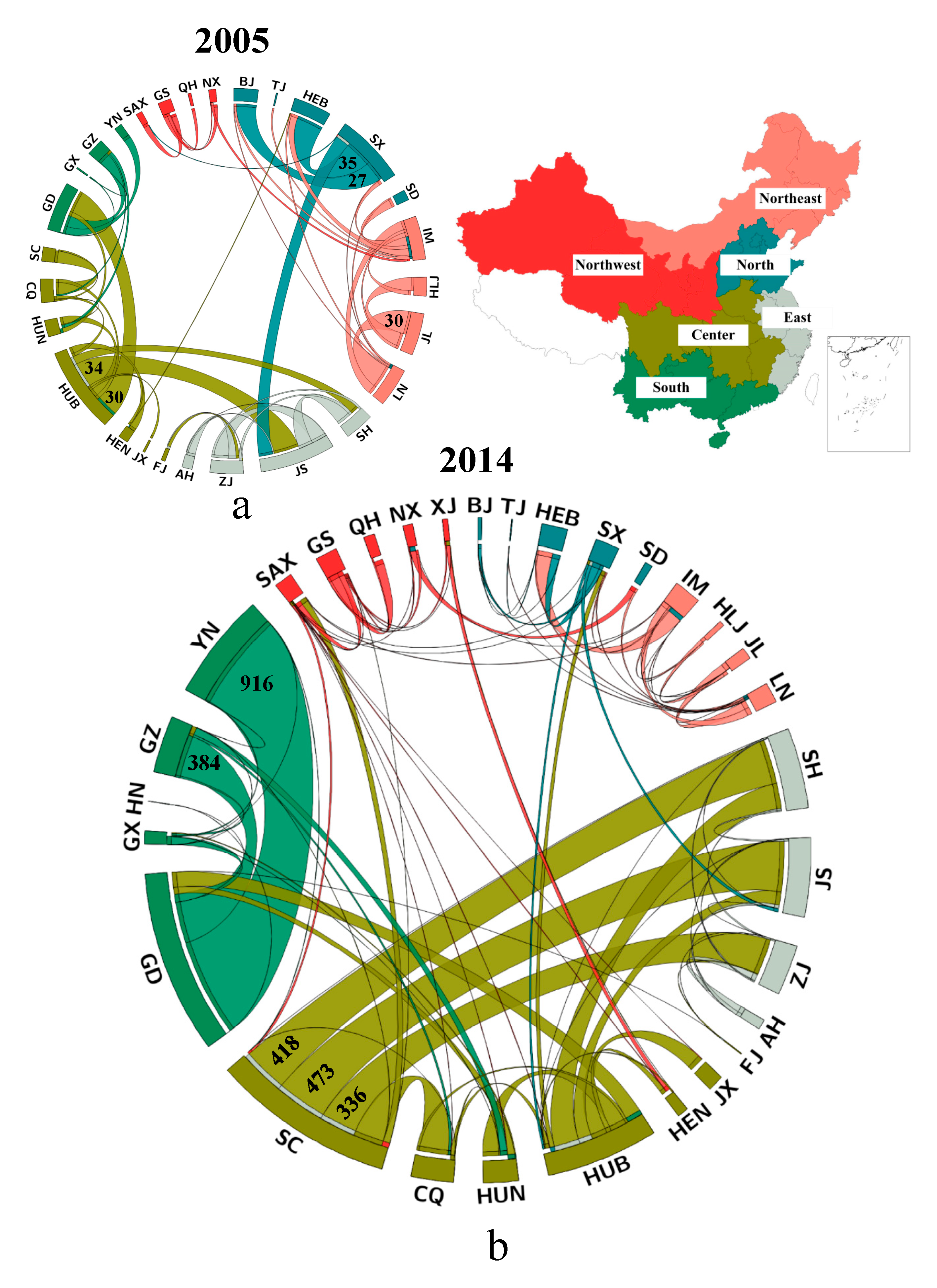
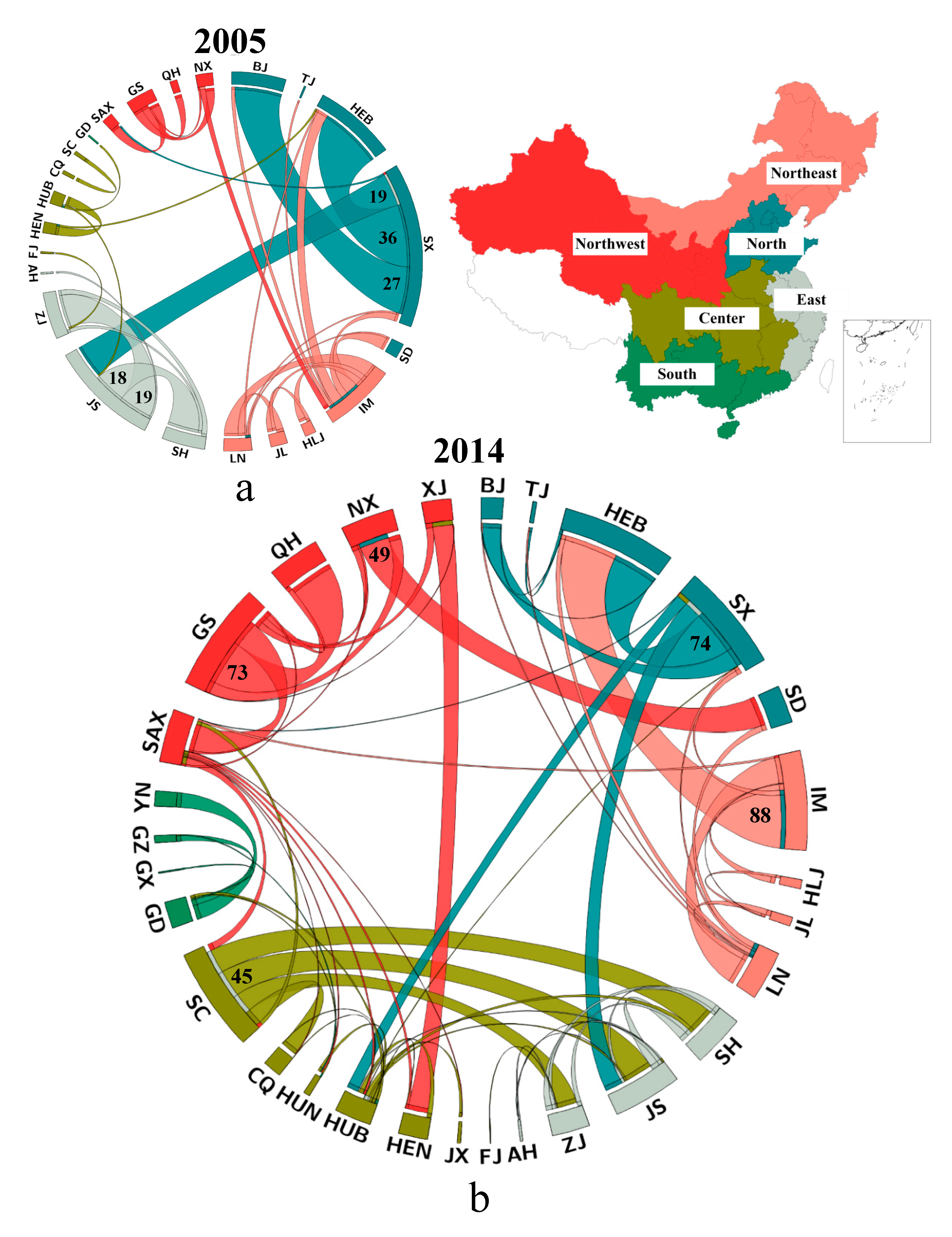
3.1. Virtual Water Transfers Embodied in Electricity Transmission

The divergence between power generation provinces and power consumption provinces are increasing, which can be represented directly by the rapidly increasing of VWT’s magnitude. The total volume of VWT increased from 450 Mm3 in 2005 to 5010 Mm3 in 2014, a factor of 11.3. As for VSWT, it increased from 204 Mm3 in 2005 to 899 Mm3 in 2014, a factor of 4.4. The different increasing speed between VWT and VSWT can be ascribed to the imbalance distribution of water resources in China. Additionally, both volumes of VWT and VSWT increased significantly than electricity transmission in the decade, which can be attributed to the expanding of hydropower that owned intensive water consumption.
Similar to the direction of electricity transmission flow, the embodied VWT mainly follows a west-to-east pattern. However, the difference between VWT and VSWT is also obvious because of the different water stress levels and power generation mix between northwestern provinces and southwestern provinces. We use the Circos tool [41] to represent the VWT network in this paper. Figure 2 shows the structure of pair-wise inter-provincial VWT in 2005 and 2014. The five largest VW flows in 2005 are Shanxi-to-Hebei (35 Mm3), Hubei-to-Jiangsu (34 Mm3), Hubei-to-Guangdong (30 Mm3), Jilin-to-Liaoning (30 Mm3), and Shanxi-to-Beijing (27 Mm3), while those flow are Yunnan-to-Guangdong (916 Mm3), Sichuan-to-Jiangsu (473 Mm3), Sichuan-to-Shanghai (418 Mm3), Guizhou-to-Guangdong (384 Mm3), and Sichuan-to-Zhejiang (336 Mm3), respectively in 2014. Those top five pair-wise flows’ summation account for 51% of all volumetric VWT. In comparison with the VWT between 2005 and 2014, southwestern provinces are playing a more and more important role in the VWT network, especially in Sichuan and Yunnan. However, the structure of VWT in the two provinces is different. In 2014, Sichuan mainly exports VW to the Yangtze River Delta, while Yunnan exports VW to Guangdong. It is ascribed to the distribution of transmission lines constructed between east to the west.
In the view of VSWT, its structure and evolution differ from the counterpart. As is shown in Figure 3, Northern provinces dominated the VWT network, while southwestern provinces are weakened. The top five VSWT flows in 2005 are Shanxi-to-Hebei (36 Mm3), Shanxi-to-Beijing (27 Mm3), Shanxi-to-Jiangsu (19 Mm3), Jiangsu-to-Zhejiang (19 Mm3), and Jiangsu-to-Shanghai (18 Mm3), while those are Inner Mongolia-to-Hebei (88 Mm3), Shanxi-to-Hebei (74 Mm3), Gansu-to-Qinghai (73 Mm3), Ningxia-to-Shandong (49 Mm3), and Sichuan-to-Jiangsu (45 Mm3), respectively, in 2014. The summation of top flows accounts for over 30% of the total VWST flows in the network. The comparison of VWT and VSWT could bring us more details. Both northwestern and southeastern provinces are main electricity exporters, but the environmental impacts posed by exporting electricity to local water resources are disproportionate because of different water stress and power generation mix in those provinces. Northeastern provinces are dominated by coal power plants, and the water scarcity in those provinces is much serious, leading to a large amount of VW and VSW run away. In contrast, southwestern provinces are water-abundant and most of the electricity is generated by hydropower plants. Thus, even the water coefficient of hydropower is large compared to thermal power, when VW adjusted to VSW, the volumes of VSW exported from southwestern provinces are very small.

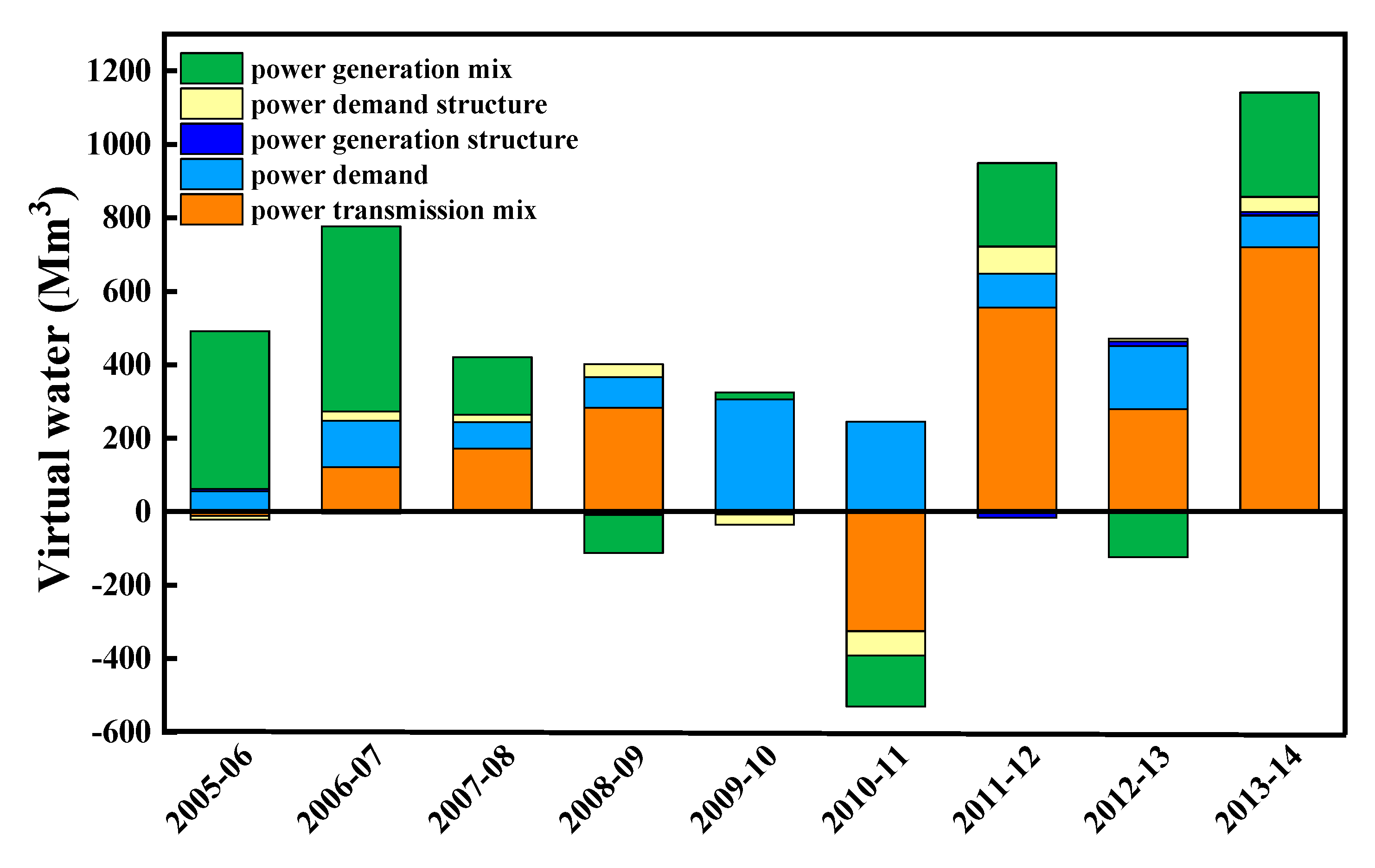
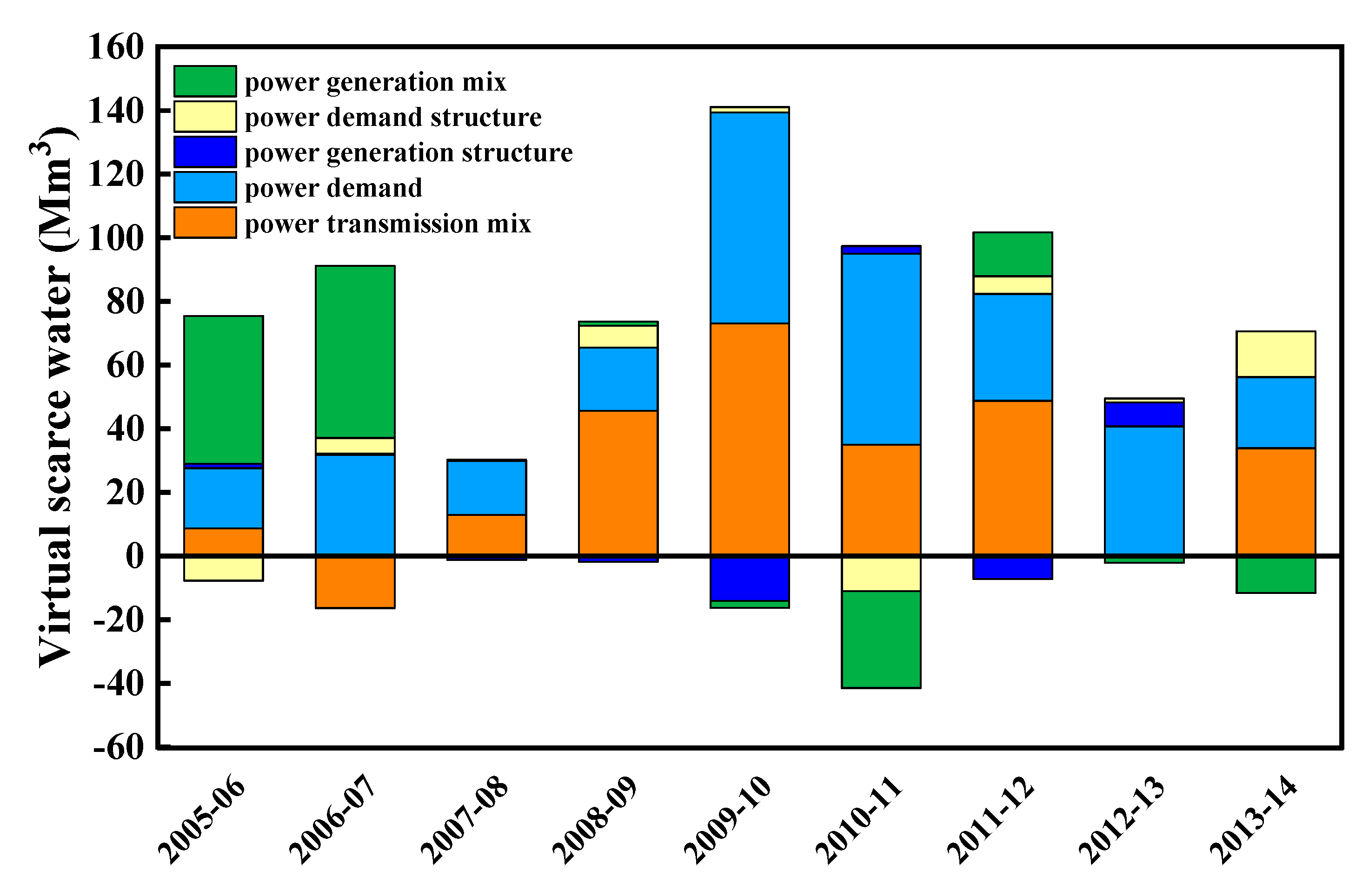
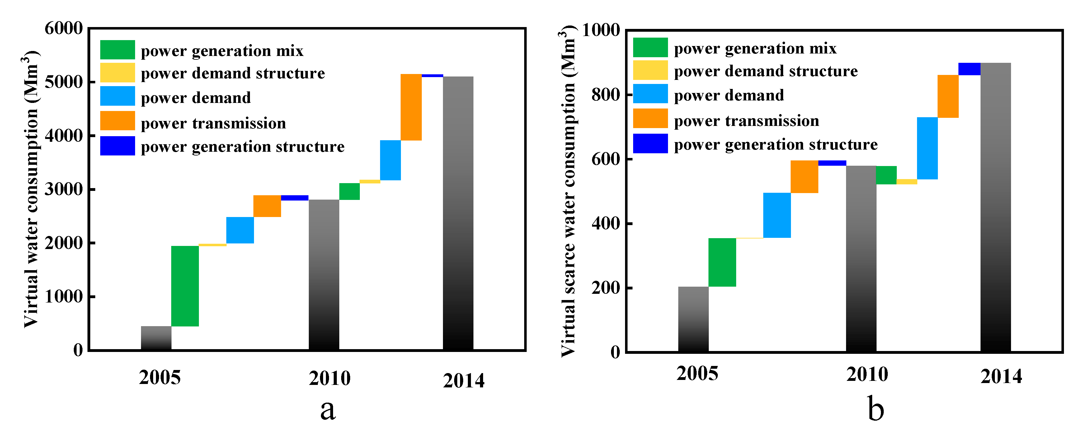
3.2. Driving Forces of Overall Virtual Water Transfers

Different driving factors (i.e., power generation mix, power transmission structure, power generation structure, power demand structure, and power demand) behind the evolution of the VWT network are determined by using a modified SDA model. Decomposition results at the national level for VWT and VSWT are illustrated in Figure 4 and Figure 5 respectively. Overall, changes in the power generation mix, power demand, and power transmission are the main drivers for the increase of VWT in 2005 to 2014. The contribution of the above-mentioned main drivers’ change differs between different periods (see Figure 4). For example, the changes in power generation mix contribute to the increase of VWT in 2005 to 2009, and then to the decrease of VWT in 2010 to 2011 and 2012 to 2013. Similar to the power generation mix, the contribution of power transmission changes is different in the decade. Excepted for the period between 2010 and 2011, the change of power transmission contributes to the increase of VWT. The change of power demand always contributes to the increase of VWT because of soaring power consumption in the decade. Furthermore, the contributions from power generation structure and power demand structure were very small compared to the other factors. This phenomenon can be ascribed to two reasons. First, although the electricity transmission increased by 3.1 times from 2005 to 2014, the power generation structure and power demand structure changed a little. In this case, the effects of power generation structure and power demand structure are limited.
In comparison with VWT, the contribution of each factor to the evolution of VSWT is different to some extent. Changes in power demand contribute most to the increase of VSWT while changes in the power generation mix and power transmission also played a vital role in leading the evolution of VSWT. In addition, the extent of effects for factors differs from different periods. For instance, the changes in the power generation mix are the main driver for the decrease of VSWT in 2011 to 2010 (−54%), and 2013 to 2014 (−19%), respectively. The contribution of changes in power transmission is very small (less than 1%) in 2012 to 2013, and it increased to a large share (57%) in 2013–2014. Additionally, changes of power demand structure and power generation structure contribute little to the evolution of VSWT, which is similar to VWT.
To clearly show different policies implemented in different periods, we divide the overall time span (2005–2014) into two periods i.e., 2005 to 2010 and 2010–2014 (see Figure 6). In the first period, the changes in power generation mix contribute most to the increase of VWT (60%) and VSWT (40%), which can be ascribed to the increasing amount of hydropower plants in this period. To reduce the air pollution of the power system, China encourages to improve the share of renewable energies, especially hydropower, as the cost of solar and wind power is expensive at that period. In the second period, the changes of power transmission (51%) are the main driver to the increase of VWT while it is power demand (61%) in VSWT. Additionally, the change of power generation mix contributes to the increase of VWT, but to the decrease of VSWT. It can be attributed to the different WSI of provinces.

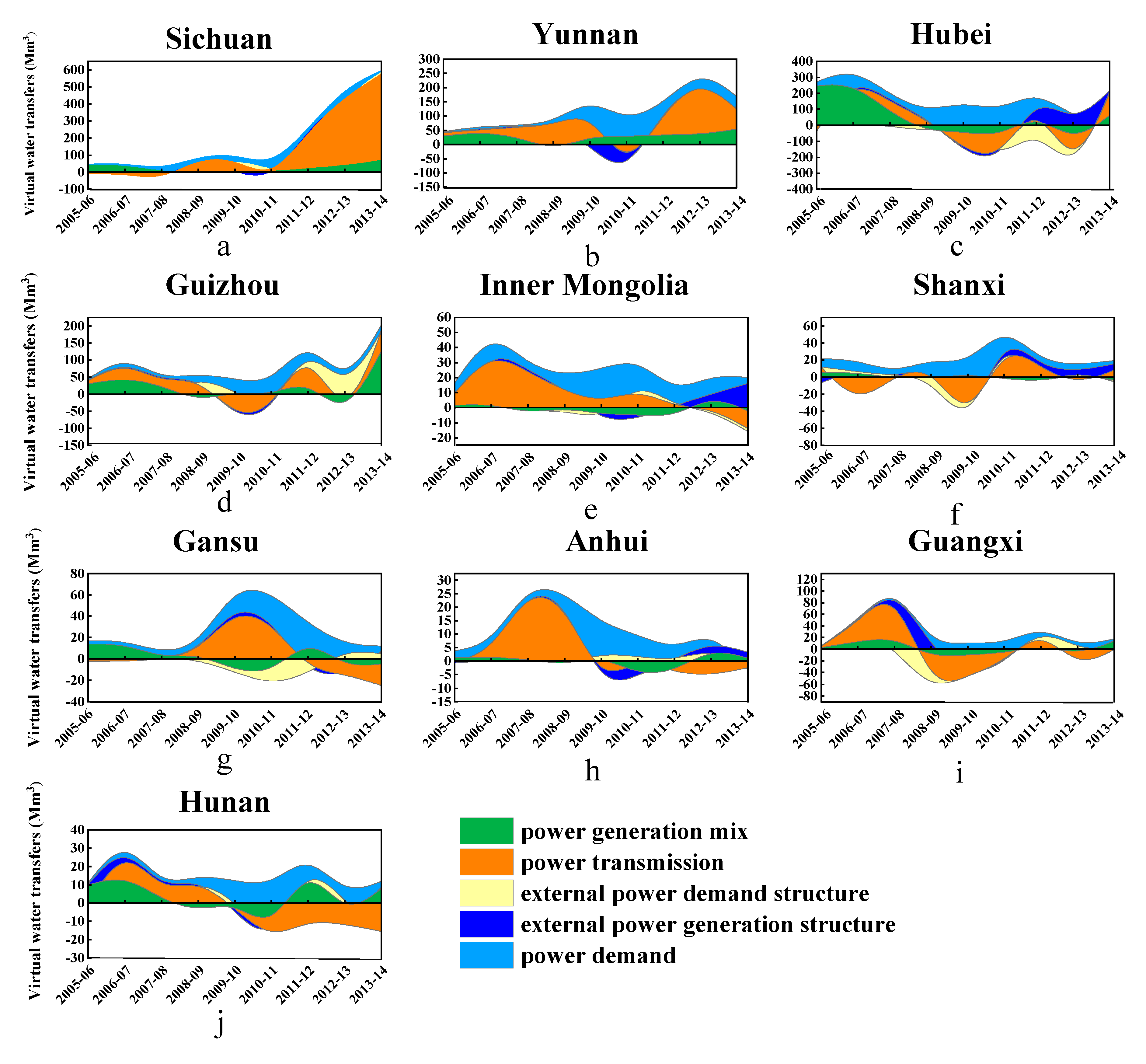
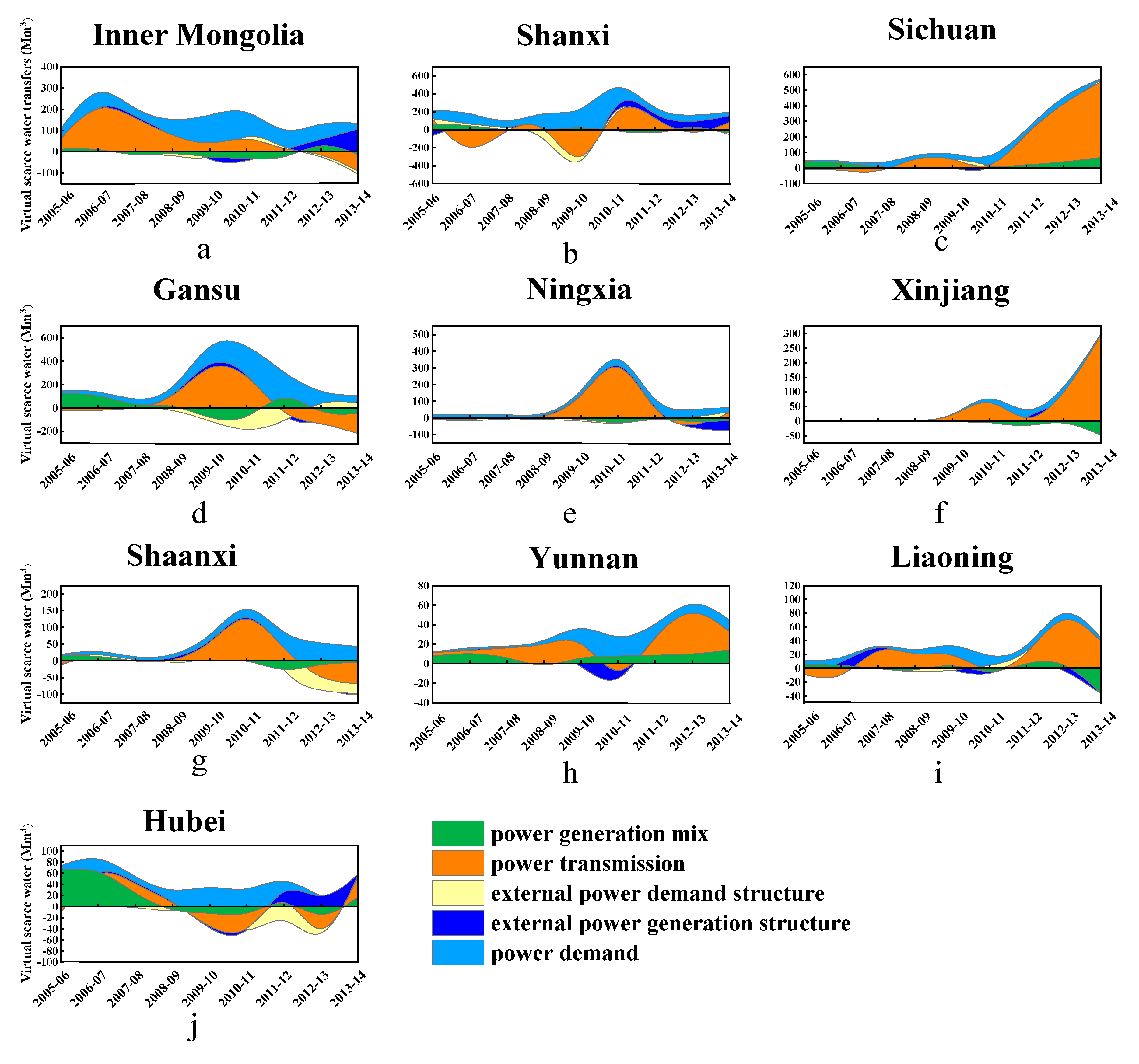
3.3. Driving Forces Analysis at the Provincial Level

The analysis at the national level reveals the overall contribution of factors to the evolution of the virtual water network but covers the details about the contribution of factors to the evolution of the virtual water network in each province. Thus, we investigated the effects of factors on the evolution of VWT and VSWT in the top ten VW and VSW exporters, respectively. The top ten VW exporters in 2014 are Sichuan, Yunnan, Hubei, Guizhou, Inner Mongolia, Shanxi, Gansu, Anhui, Guangxi, and Hunan, in which the VW exporting accounts for 91% of the total VWT. Additionally, at the provincial level, power generation structure and power demand structure should be considered as external power generation structure and external power demand structure based on modified SDA [32].
The factor decomposition results for the top ten VW exporters from 2005 to 2014 are shown in Figure 7. The contributions of factors differ from various provinces and periods. Generally, power demand, power transmission and power generation mix jointly determined the evolution of the VWT network. Sichuan is the largest VW exporter in 2014. In Sichuan, the changes in power generation mix (114%, 104%) dominated the increase of VWT in 2005–2006 and 2006–2007, while the changes of power transmission contribute mostly to the increase of VWT between 2011–2012 (89%) and 2013–2014 (85%). Excepted Sichuan, the same condition occurs in other southwestern exporters such as Hubei, Yunnan, and Guizhou. In those provinces, the power transmission is the main driver of the increase of VWT (see Figure 7) in some periods, but it can be the main driver of the decrease of VWT in other periods. For example, in the 2009–2010 and 2010–2011 periods, the power transmission contributes mostly to the decrease of VWT in Hubei. Compared to southwestern exporters, northwestern exporters show some different characters. Power transmission dominated the change of VWT, which is similar to the southwestern provinces, but the change of power demand replaced the power generation mix and contributes to the second-largest increase of VWT. Especially, between 2013 to 2014, the change of external power generation structure (36%) contributes to the most increase in Inner Mongolia while the change of power transmission is the main driver (25.9%) of the VWT’s decrease.
The top ten VSW exporters are Inner Mongolia, Shanxi, Sichuan, Gansu, Ningxia, Xinjiang, Shaanxi, Yunnan, Liaoning, and Hubei, in which the accumulation of VSW accounts for 88.9% of the total VSWT. Figure 8 shows the decomposition results of the VSWT network. The contribution of each factor differs from different periods and provinces. Inner Mongolia is the largest VSW exporter in 2014, and the power transmission contributes mostly to the increase of the VSWT between 2005 to 2009, but it is replaced by power demand in other periods. Similar to the VWT evolution, power generation mix, and power transmission play different roles in different periods. As for the change of external power generation structure and external power demand structure, it generally plays a small role in driving the change of VSWT. However, the change of external power generation structure contributes largely to the change of VSWT in a specific period. For example, it contributes mostly to the increase of VSWT in Inner Mongolia between 2013 and 2014, but to the decrease of VSWT in Ningxia between 2013 and 2014.
To further investigate the impacts posed by different policies on the evolution of VSWT, we further divided the decade into two periods, i.e., 2005 to 2010 and 2010 to 2014. Figure 9 shows the contributions of factors for the top ten VW and VSW exporters in the two periods. In the first period (here is 2005 to 2010), the power generation mix and power transmission are the main drivers to the change of VWT. In the second period (here is 2010–2014), power demand and power transmission contribute mostly to the change of VWT. However, the change of power transmission in one province (i.e., Shanxi) plays a negative role in the change of VWT in the first period, while it increased to five provinces in the second province. This phenomenon can be ascribed to the evolution of the transmission structure. In comparison with the first period, the power generation structure and the power demand structure play a more important role in the second period, especially in Inner Mongolia and Anhui.
Figure 9 also shows the decomposition results for the top ten VSW exporters in the two periods. In the first decade, Inner Mongolia is the largest VSW exporter, and the change of power transmission (64%) contributes mostly to the increase of VSWT. In the second decade, the power demand replaced the power transmission and plays the largest positive role (75%) in the evolution of VSWT in Inner Mongolia. The transform between the two periods can be ascribed to the different policies implemented in different periods. Especially, in the first period, the change of power transmission contributes mostly to the decrease of VWT and VSWT in Shanxi. In the second period, the power generation mix is the main driver of the VSWT’s decrease in Hubei.

4. Discussion

4.1. Impacts of Policies to the Virtual Water Transmission

The evolution of the virtual water network embodied in China’s power system was impacted by different policies implemented over periods. The decomposition model identified the change of power generation mix was a major factor impacting the evolution of VWT from 2005 to 2010 (Figure 9). The high proportion of thermal power generation has induced serious air pollution and made negative effects on climate change. The construction of hydropower plants was promoted to meet the power demand of developed regions. During the first period, the power generation from hydropower had increased from 397 TWh to 722 TWh, with a factor of 1.8. However, the water coefficient of hydropower is higher than that of thermal power, which drives more virtual water delivered from southwestern areas to load hubs concentrated in northeastern areas.
The power transmission and power demand are important factors that increased the virtual water transfers in the second period (2010–2014). They attributed to the increase of investment in power transmission lines. The maturity of UHV technologies exceeded the construction of the UHV-power transmission line. In the period, UHV electricity transmission in China had developed rapidly in relation to the long-distance transmission of alternating current and direct current electricity. In 2010, the 1000-kV Nanyang-Jingmen UHV AC project and the 800 kV UHV DC Yunnan-Guangdong project were put into operation. Besides, the 800 kV UHV DC transmission line from Xiangjiaba to Shanghai commenced operation. The UHV transmission project from Jinping to Southern Jiangsu was put into operation in 2012. The expand of transmission capacity made the power grid more feasible and released the hydropower potential of southeastern provinces, including Yunnan, Sichuan, Hubei, and Guizhou. The change of power transmission dominated the increase of VWT at national level, but that was the main driver of the decrease of VWT in terms of the individual province (e.g., Hubei). Even the overall transmission capacity increased, the amount of power transmission from Hubei significantly decreased in this period. It is noted that the power transmission directly from Sichuan and Guizhou can satisfy the power demand in Guangdong and Yangtze River Delta, which was one reason for the decrease of power export in Hubei. The contributions from the changes in power generation and demand structure were little when compared with the aforementioned factors. It can be referred that power generation and demand structure change had no direct relationship with power transmission change.

4.2. Advice for the Development of China’s Power System

Centralized spatial distribution of power generation and investment on the UHV project has led to the diverging between power generation and consumption. Driven by the soaring electricity consumption in load hubs, the magnitudes of electricity transmission will continuously increase in the future. For load hubs, importing electricity from western provinces could mitigate their water stress and air pollution, especially the already polluted Jing-Jin-Jiarea [42]. In the view of power generation provinces, exporting electricity can release their power generation potential and develop the local economy. However, the expanding of electricity transmission increasingly reallocated water resources in both the generation side and consumption side, which may aggravate the water scarcity in China because of the mismatch between water resources and energy resources.
We explored the evolution of VW transfers embodied in provincial electricity transmission and identified the related driving factors. According to the results, a large amount of VW was transferred from western to the eastern provinces, which exacerbated the water stress in western provinces. The water consumption of power plants competed with the water consumption of urbanization and agriculture. Many VW exporters suffering serious hydrological challenges [43]. For instance, Inner Mongolia exported VW to Jing-Ji-Jin area for decades, but Inner Mongolia faced high water stress pressure and the challenge of groundwater depletion. Exporting VW from Inner Mongolia exacerbated the conflicts between different sectors. Some northeastern exporters (i.e., Shanxi, Shaanxi, Ningxia, Xinjiang, and Gansu) facing the same conditions. The power-related VW in southwestern areas was mainly delivered to the Yangtze River Delta and Guangdong. In comparison with northwestern provinces dominated by thermal power, hydropower played a vital role in the southwestern provinces. The transfer of VW in hydroelectricity did not pose water stress to the local ecosystem because of rich abundant water resources in southwestern provinces. The transmission pattern of southeastern provinces is thus more positive than that of northeastern provinces.
Considering the competition for the demands of water resources among energy, urban consumption, and agriculture sectors [44], we suggest that policymakers should integrate across the water-electricity nexus at regional and national levels. To reduce the water pressure in China, the government issued the stringent regulation in 2012, which constrained the national freshwater withdrawals into a definite magnitude (670 billion Mm3). Although water-saving measures have been implemented on a single plant or sector, synergetic management taking water-electricity nexus into account has not yet been implemented by the government.
Instead of the water scarcity, other environmental impacts (e.g., carbon emission, air pollution, etc.) induced by power systems has raised attention worldwide as well [45]. How to deal with those problems with new technologies (renewable energies connecting technology, artificial intelligence technology, etc.) is associated with the development of power grids. Improving the share of renewable energies is a highlighted way to reduce pollution and emission.

4.3. Advantages and Limitations

This study constructed a virtual water network and explored its evolution, based on the long-time series of electricity transmission data. Compared to previous studies using MRIO tables [30], we directly used the power transmission table, which could avoid the bias from sector aggregation and monetary inhomogeneity in MRIO analysis. The water intensity data for power generation technologies dismissed the impacts of spatial distribution. For example, the special climate is various, and different temperatures and wind speed influence the water evaporation of the reservoir. Moreover, the water coefficient for thermal power plants had been reduced with the improvement of cooling systems in the decade [37].

5. Conclusions

This study investigated the dynamics of the virtual water network embodied in the interprovincial electricity transmission in China and identified its driving factors in different periods by dividing the decade into the two-periods of 2005–2010 and 2010–2014. First, the transfer of virtual water and virtual scarce water generally followed a west-to-east pattern, and their magnitude increased rapidly because of the soaring electricity demand. Considering spatial distribution, virtual water exporters deeply influenced the virtual scarce water network, because of various water stress degree. The export of virtual scarce water in northwestern areas was mainly driven by electricity consumption in Jing-Jin-Ji area, and it was mainly driven by electricity consumption in southeastern areas (e.g., Yangtze River Delta and Guangdong). Besides, the newly constructed transmission lines between Xinjiang and Henan made the Xinjiang-to-Henan virtual scarce water flow increased significantly. According to the water endowments in southeastern provinces and northwestern provinces, the virtual water transmission from southeastern provinces benefits the overall water resources, but that from northwestern provinces would aggravate regional water scarcity. Increasingly developed hydropower generation in the southeastern province can mitigate water scarcity in China even it is water-intensive.
The contribution of driving factors differs from different periods because of the implemental effects of policies. At the national level, the change of power generation mix dominated the increase of the virtual water network in the first period (2005–2010), while the change of power transmission dominated the increase in the second period. At the provincial level, power generation mix and power transmission were the main drivers of the change of virtual water transfers in the top ten provinces. Considering the development trend of the power system in the future, the investigation for co-benefits of dealing with different environmental impacts should be highlighted.

Supplementary Materials

The following are available online at https://www.mdpi.com/1996-1073/13/2/328/s1.

Author Contributions

Conceptualization, Y.Z. and S.H.; Methodology, S.H.; Investigation, S.H. and J.W.; Writing—Original Draft, S.H.; Writing—Review & Editing, J.W., Y.Z. and J.L.; Funding Acquisition, J.L. and H.Z.; Resources, C.Z.; Supervision, J.L. All authors have read and agreed to the published version of the manuscript.

Funding

This work was supported by the National Natural Science Foundation of China (51867003), the Basic Ability Promotion Project for Yong Teachers in Universities of Guangxi (2019KY0046; 2019KY0022), the Natural Science Foundation of Guangxi (2018JJB160056; 2018JJB160064; 2018JJA160176), the Guangxi thousand backbone teachers training program, the boshike award scheme for young innovative talents, and the Guangxi bagui young scholars special funding.

Conflicts of Interest

The authors declare no conflict of interest.

References

  1. Fang, D.; Chen, B. Linkage analysis for water-carbon nexus in China. Appl. Energy 2018, 225, 682–695. [Google Scholar] [CrossRef]
  2. Larsen, M.A.D.; Drews, M. Water use in electricity generation for water-energy nexus analyses: The European case. Sci. Total Environ. 2019, 651, 2044–2058. [Google Scholar] [CrossRef] [PubMed]
  3. Li, J.S.; Chen, G.Q. Water footprint assessment for service sector: A case study of gaming industry in water scarce Macao. Ecol. Indic. 2014, 47, 164–170. [Google Scholar] [CrossRef]
  4. China State Council (CSC). Opinions of the State Council on the Implementation of the Strictest Water Resources Management System. 2012. Available online: http://www.gov.cn/zwgk/2012-02/16/content_2067664.htm (accessed on 18 December 2019).
  5. Ministry of Water Resources of China. China Water Resources Bulletin in 2018. Available online: http://www.gov.cn/xinwen/2019-07/13/content_5408959.htm (accessed on 18 December 2019).
  6. Cai, B.; Zhang, B.; Bi, J.; Zhang, W. Energy’s Thirst for Water in China. Environ. Sci. Technol. 2014, 48, 11760–11768. [Google Scholar] [CrossRef] [PubMed]
  7. Nogueira Vilanova, M.R.; Perrella Balestieri, J.A. Exploring the water-energy nexus in Brazil: The electricity use for water supply. Energy 2015, 85, 415–432. [Google Scholar] [CrossRef]
  8. Farfan, J.; Breyer, C. Combining Floating Solar Photovoltaic Power Plants and Hydropower Reservoirs: A Virtual Battery of Great Global Potential. Energy Procedia 2018, 155, 403–411. [Google Scholar] [CrossRef]
  9. Zhang, J.; Lei, X.; Chen, B.; Song, Y. Analysis of blue water footprint of hydropower considering allocation coefficients for multi-purpose reservoirs. Energy 2019, 188, 116086. [Google Scholar] [CrossRef]
  10. Zaunbrecher, B.S.; Daniels, B.; Roß-Nickoll, M.; Ziefle, M. The social and ecological footprint of renewable power generation plants. Balancing social requirements and ecological impacts in an integrated approach. Energy Res. Soc. Sci. 2018, 45, 91–106. [Google Scholar] [CrossRef]
  11. Sharifzadeh, M.; Hien, R.K.T.; Shah, N. China’s roadmap to low-carbon electricity and water: Disentangling greenhouse gas (GHG) emissions from electricity-water nexus via renewable wind and solar power generation, and carbon capture and storage. Appl. Energy 2019, 235, 31–42. [Google Scholar] [CrossRef] [Green Version]
  12. He, G.; Zhao, Y.; Jiang, S.; Zhu, Y.; Li, H.; Wang, L. Impact of virtual water transfer among electric sub-grids on China’s water sustainable developments in 2016, 2030, and 2050. J. Clean. Prod. 2019, 239, 118056. [Google Scholar] [CrossRef]
  13. Murrant, D.; Quinn, A.; Chapman, L.; Heaton, C. Water use of the UK thermal electricity generation fleet by 2050: Part 1 identifying the problem. Energy Policy 2017, 108, 844–858. [Google Scholar] [CrossRef]
  14. Murrant, D.; Quinn, A.; Chapman, L.; Heaton, C. Water use of the UK thermal electricity generation fleet by 2050: Part 2 quantifying the problem. Energy Policy 2017, 108, 859–874. [Google Scholar] [CrossRef]
  15. Allan, J.A. Virtual Water: A Strategic Resource Global Solutions to Regional Deficits. Groundwater 1998, 36, 545–546. [Google Scholar] [CrossRef]
  16. Allan, T. (School of O and AS.) Fortunately there are substitutes for water: Otherwise our hydropolitical futures would be impossible. In Bibliographic Information; Overseas Development Administration: London, UK, 1993. [Google Scholar]
  17. Feng, K.; Hubacek, K.; Siu, Y.L.; Li, X. The energy and water nexus in Chinese electricity production: A hybrid life cycle analysis. Renew. Sustain. Energy Rev. 2014, 39, 342–355. [Google Scholar] [CrossRef] [Green Version]
  18. Pfister, S.; Saner, D.; Koehler, A. The environmental relevance of freshwater consumption in global power production. Int. J. Life Cycle Assess. 2011, 16, 580–591. [Google Scholar] [CrossRef] [Green Version]
  19. Zhang, C.; Anadon, L.D. Life Cycle Water Use of Energy Production and Its Environmental Impacts in China. Environ. Sci. Technol. 2013, 47, 14459–14467. [Google Scholar] [CrossRef] [Green Version]
  20. Zhu, X.; Guo, R.; Chen, B.; Zhang, J.; Hayat, T.; Alsaedi, A. Embodiment of virtual water of power generation in the electric power system in China. Appl. Energy 2015, 151, 345–354. [Google Scholar] [CrossRef]
  21. Guo, R.; Zhu, X.; Chen, B.; Yue, Y. Ecological network analysis of the virtual water network within China’s electric power system during 2007–2012. Appl. Energy 2016, 168, 110–121. [Google Scholar] [CrossRef]
  22. Zhang, C.; Zhong, L.; Liang, S.; Sanders, K.T.; Wang, J.; Xu, M. Virtual scarce water embodied in inter-provincial electricity transmission in China. Appl. Energy 2017, 187, 438–448. [Google Scholar] [CrossRef] [Green Version]
  23. Chini, C.M.; Djehdian, L.A.; Lubega, W.N.; Stillwell, A.S. Virtual water transfers of the US electric grid. Nat. Energy 2018, 3, 1115–1123. [Google Scholar] [CrossRef]
  24. Zhang, Y.Y.; Fang, J.K.; Wang, S.G.; Yao, H. Energy-water nexus in electricity trade network: A case study of interprovincial electricity trade in China. Appl. Energy 2020, 257, 113685. [Google Scholar] [CrossRef]
  25. NDRC (National Development and Reform Commission); NEA (National Energy Administration). Energy Production and Consumption Revolution Strategy; NDRC and NEA: Beijing, China, 2016. Available online: http://www.ndrc.gov.cn/gzdt/201704/t20170425_845304.html (accessed on 18 December 2019).
  26. Yan, D.; Lei, Y.; Li, L. Driving Factor Analysis of Carbon Emissions in China’s Power Sector for Low-Carbon Economy. Math. Probl. Eng. 2017, 2017, 4954217. [Google Scholar] [CrossRef] [Green Version]
  27. Hoekstra, R.; van den Bergh, J.C.J.M. Comparing structural decomposition analysis and index. Energy Econ. 2003, 25, 39–64. [Google Scholar] [CrossRef]
  28. Goh, T.; Ang, B.W.; Su, B.; Wang, H. Drivers of stagnating global carbon intensity of electricity and the way forward. Energy Policy 2018, 113, 149–156. [Google Scholar] [CrossRef]
  29. Liao, X.; Hall, J.W. Drivers of water use in China’s electric power sector from 2000 to 2015. Environ. Res. Lett. 2018, 13, 094010. [Google Scholar] [CrossRef]
  30. Zhang, Y.; Chen, Q.; Chen, B.; Liu, J.; Zheng, H.; Yao, H.; Zhang, C. Identifying hotspots of sectors and supply chain paths for electricity conservation in China. J. Clean. Prod. 2020, 251, 119653. [Google Scholar] [CrossRef]
  31. Cai, B.; Zhang, W.; Hubacek, K.; Feng, K.; Li, Z.; Liu, Y.W.; Liu, Y. Drivers of virtual water flows on regional water scarcity in China. J. Clean. Prod. 2019, 207, 1112–1122. [Google Scholar] [CrossRef]
  32. Wang, S.; Zhu, X.; Song, D.; Wen, Z.; Chen, B.; Feng, K. Drivers of CO2 emissions from power generation in China based on modified structural decomposition analysis. J. Clean. Prod. 2019, 220, 1143–1155. [Google Scholar] [CrossRef]
  33. Zhang, C.; He, G.; Zhang, Q.; Liang, S.; Zipper, S.C.; Guo, R.; Zhao, X.; Zhong, L.; Wang, J. The evolution of virtual water flows in China’s electricity transmission network and its driving forces. J. Clean. Prod. 2020, 242, 118336. [Google Scholar] [CrossRef]
  34. Dietzenbacher, E.; Los, B. Structural Decomposition Techniques: Sense and Sensitivity. Econ. Syst. Res. 1998, 10, 307–324. [Google Scholar] [CrossRef]
  35. NDRC (National Development and Reform Commission). The 13th Five-Year (2016–2020) Development Plan for Electric Power Industry; NDRC: Beijing, China, 2017. Available online: https://en.ndrc.gov.cn/ (accessed on 18 December 2019).
  36. Liu, M.; Huang, Y.; Ma, Z.; Jin, Z.; Liu, X.; Wang, H.; Liu, Y.; Wang, J.; Jantunen, M.; Bi, J.; et al. Spatial and temporal trends in the mortality burden of air pollution in China: 2004–2012. Environ. Int. 2017, 98, 75–81. [Google Scholar] [CrossRef] [PubMed] [Green Version]
  37. Zhang, C.; Zhong, L.; Wang, J. Decoupling between water use and thermoelectric power generation growth in China. Nat. Energy 2018, 3, 792–799. [Google Scholar] [CrossRef]
  38. CEC (China Electricity Council). Annual Compilation of Statistics of Power Industry; China Electricity Council: Beijing, China, 2005–2014. (In Chinese) [Google Scholar]
  39. Li, X.; Feng, K.; Siu, Y.L.; Hubacek, K. Energy-water nexus of wind power in China: The balancing act between CO2 emissions and water consumption. Energy Policy 2012, 45, 440–448. [Google Scholar] [CrossRef]
  40. Pfister, S.; Koehler, A.; Hellweg, S. Assessing the Environmental Impacts of Freshwater Consumption in LCA. Environ. Sci. Technol. 2009, 43, 4098–4104. [Google Scholar] [CrossRef] [PubMed] [Green Version]
  41. Krzywinski, M.; Schein, J.; Birol, İ.; Connors, J.; Gascoyne, R.; Horsman, D.; Jones, S.J.; Marra, M.A. Circos: An information aesthetic for comparative genomics. Genome Res. 2009, 19, 1639–1645. [Google Scholar] [CrossRef] [Green Version]
  42. Wang, Y.; Li, M.; Wang, L.; Wang, H.; Zeng, M.; Zeng, B.; Qiu, F.; Sun, C. Can remotely delivered electricity really alleviate smog? An assessment of China’s use of ultra-high voltage transmission for air pollution prevention and control. J. Clean. Prod. 2020, 242, 118430. [Google Scholar] [CrossRef]
  43. Liao, X.; Chai, L.; Xu, X.; Lu, Q.; Ji, J. Grey water footprint and interprovincial virtual grey water transfers for China’s final electricity demands. J. Clean. Prod. 2019, 227, 111–118. [Google Scholar] [CrossRef]
  44. Chen, B.; Han, M.Y.; Peng, K.; Zhou, S.L.; Shao, L.; Wu, X.F.; Wei, W.D.; Liu, S.Y.; Li, Z.; Li, J.S.; et al. Global land-water nexus: Agricultural land and freshwater use embodied in worldwide supply chains. Sci. Total Environ. 2018, 613–614, 931–943. [Google Scholar] [CrossRef]
  45. Guo, Y.; Chen, B.; Li, J.; Yang, Q.; Wu, Z.; Tang, X. The evolution of China’s provincial shared producer and consumer responsibilities for energy-related mercury emissions. J. Clean. Prod. 2019, 245, 118678. [Google Scholar] [CrossRef]
Figure 1. The water stress index (WSI) and electricity generation mix of each province in 2014.
Energies 13 00328 g001
Figure 2. Pair-wise virtual water flows between provinces in 2005 (a), and 2014 (b). The top five flows are labeled. The color of the ribbon represents the different subnational grid. The ribbon touches inner circle refers to the export, while out of touch means an import. AH―Anhui, BJ―Beijing, CQ―Chongqing, FJ―Fujian, GD―Guangdong, GS―Gansu, GX―Guangxi, GZ―Guizhou, HEB―Hebei, HEN―Henan, HLJ―Heilongjiang, HUB―Hubei, HUN―Hunan, IM―Inner Mongolia, JL―Jilin, JS―Jiangsu, JX―Jiangxi, LN―Liaoning, NX―Ningxia, QH―Qinghai, SAX―Shaanxi, SC―Sichuan, SD―Shandong, SH―Shanghai, SX―Shanxi, TJ―Tianjin, XJ―Xinjiang, YN―Yunnan, ZJ―Zhejiang.
Energies 13 00328 g002
Figure 3. Pair-wise virtual scarce water flows between provinces in 2005 (a), and 2014 (b). The top five flows are labeled. The color of the ribbon represents the different subnational grid. The ribbon touches inner circle refers to the export, while out of touch means an import. AH―Anhui, BJ―Beijing, CQ―Chongqing, FJ―Fujian, GD―Guangdong, GS―Gansu, GX―Guangxi, GZ―Guizhou, HEB―Hebei, HEN―Henan, HLJ―Heilongjiang, HUB―Hubei, HUN―Hunan, IM―Inner Mongolia, JL―Jilin, JS―Jiangsu, JX―Jiangxi, LN―Liaoning, NX―Ningxia, QH―Qinghai, SAX―Shaanxi, SC―Sichuan, SD―Shandong, SH―Shanghai, SX―Shanxi, TJ―Tianjin, XJ―Xinjiang, YN―Yunnan, ZJ―Zhejiang.
Energies 13 00328 g003
Figure 4. The contribution of driving factors to the changes of virtual water transmission.
Energies 13 00328 g004
Figure 5. The contribution of driving factors to the changes of virtual scarce water transmission.
Energies 13 00328 g005
Figure 6. The contribution of different factors to the change of (a) virtual water transmission; (b) virtual scarce water transmission.
Energies 13 00328 g006
Figure 7. (aj) The contribution of driving factors to the change of virtual water transmission in the top ten virtual water exporters in 2014.
Energies 13 00328 g007
Figure 8. (aj) The contribution of driving factors to the evolution of virtual scarce water transmission in the top ten exporters in 2014.
Energies 13 00328 g008
Figure 9. The evolution of virtual water transmission (a,b), and virtual scarce water transmission (c,d) of top ten provinces in two periods.
Energies 13 00328 g009

