Dynamic Tariff for Day-Ahead Congestion Management in Agent-Based LV Distribution Networks


Abstract
1. Introduction
- Day-ahead market-based congestion management through agent-based scheduling of the residential appliances;
- The estimated incurred cost of overloading is determined through the dynamic loading model of the transformer and used as the trigger for the procurement of flexibility;
- The dynamic network tariff has been calculated through a robust formulation considering uncertainties in loading and correlation among loading in different time steps.
2. Approach
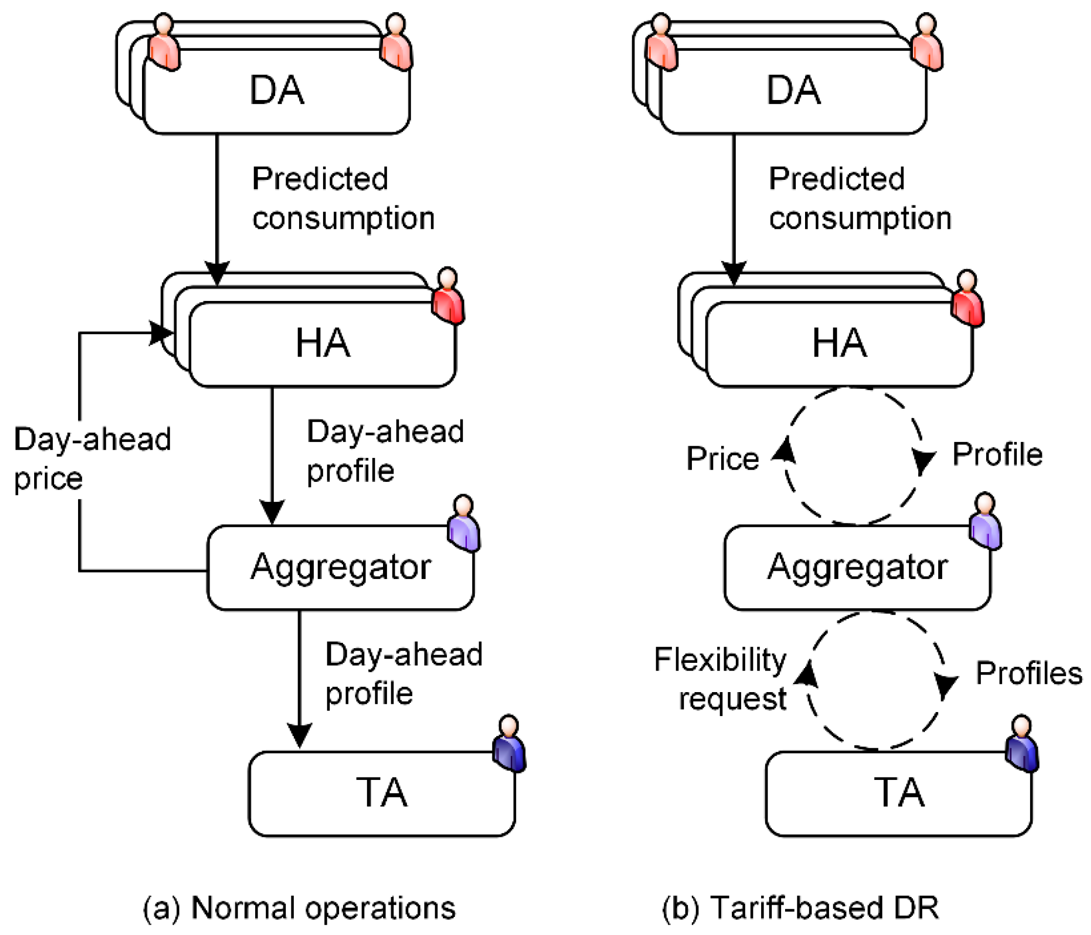
2.1. Overview
2.2. MAS-Based System Architecture
3. Modeling
3.1. Response to Dynamic Pricing
3.2. Price Adjustments
3.2.1. Overloading Cost of the Transformer
3.2.2. Calculation of Dynamic Tariff
4. Simulation Setup
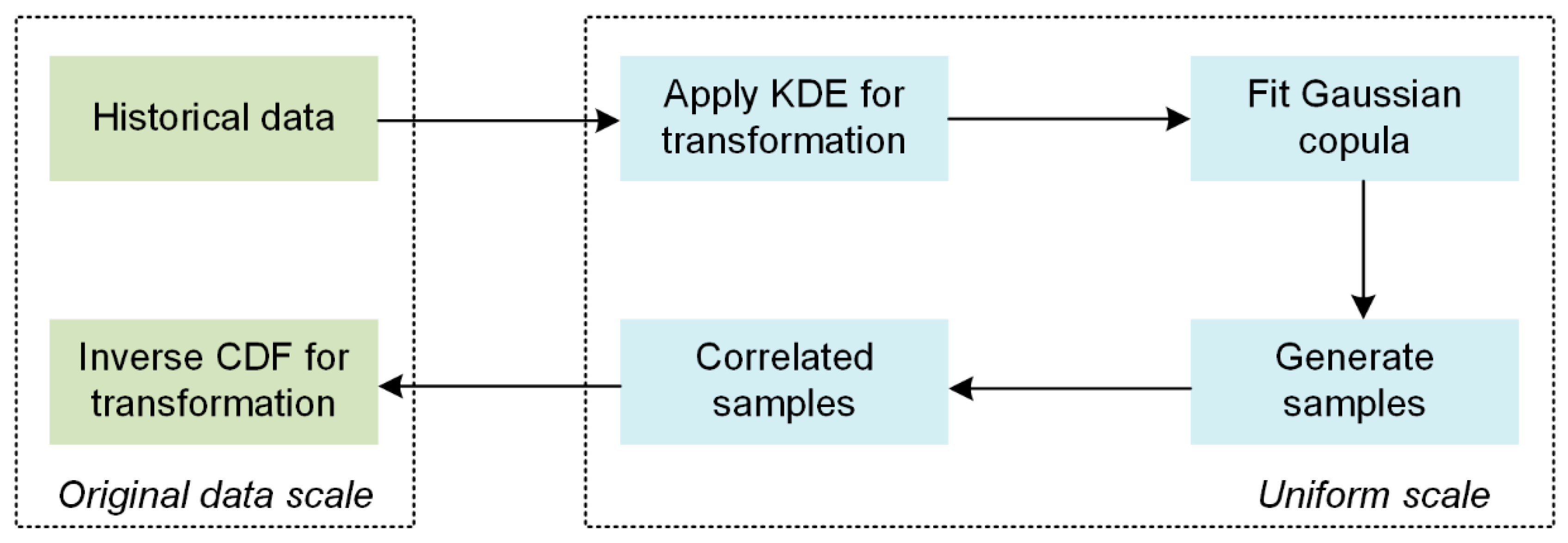
4.1. Load Modeling
4.2. Network
4.3. Simulation Platform
5. Numerical Results
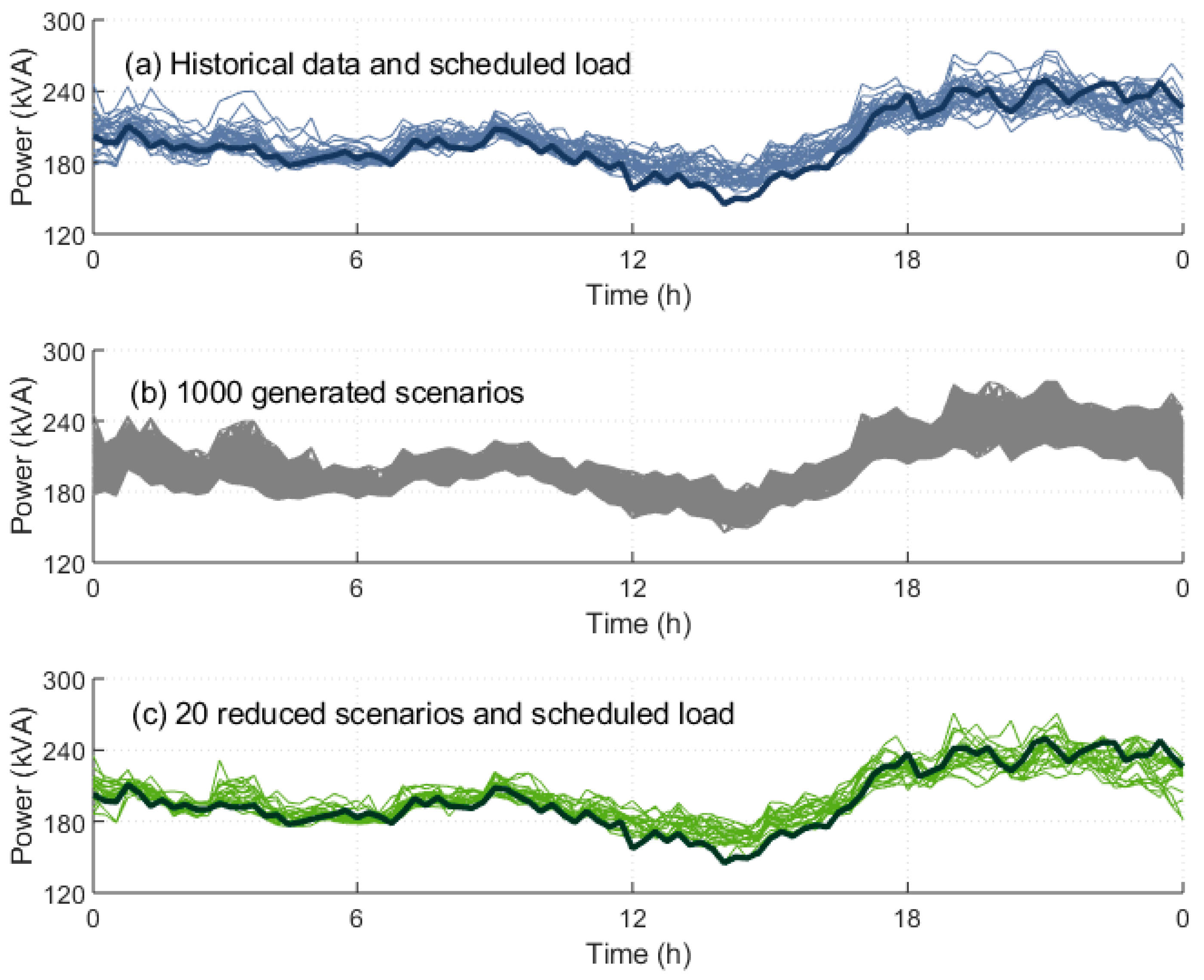
5.1. Scenarios of Loading
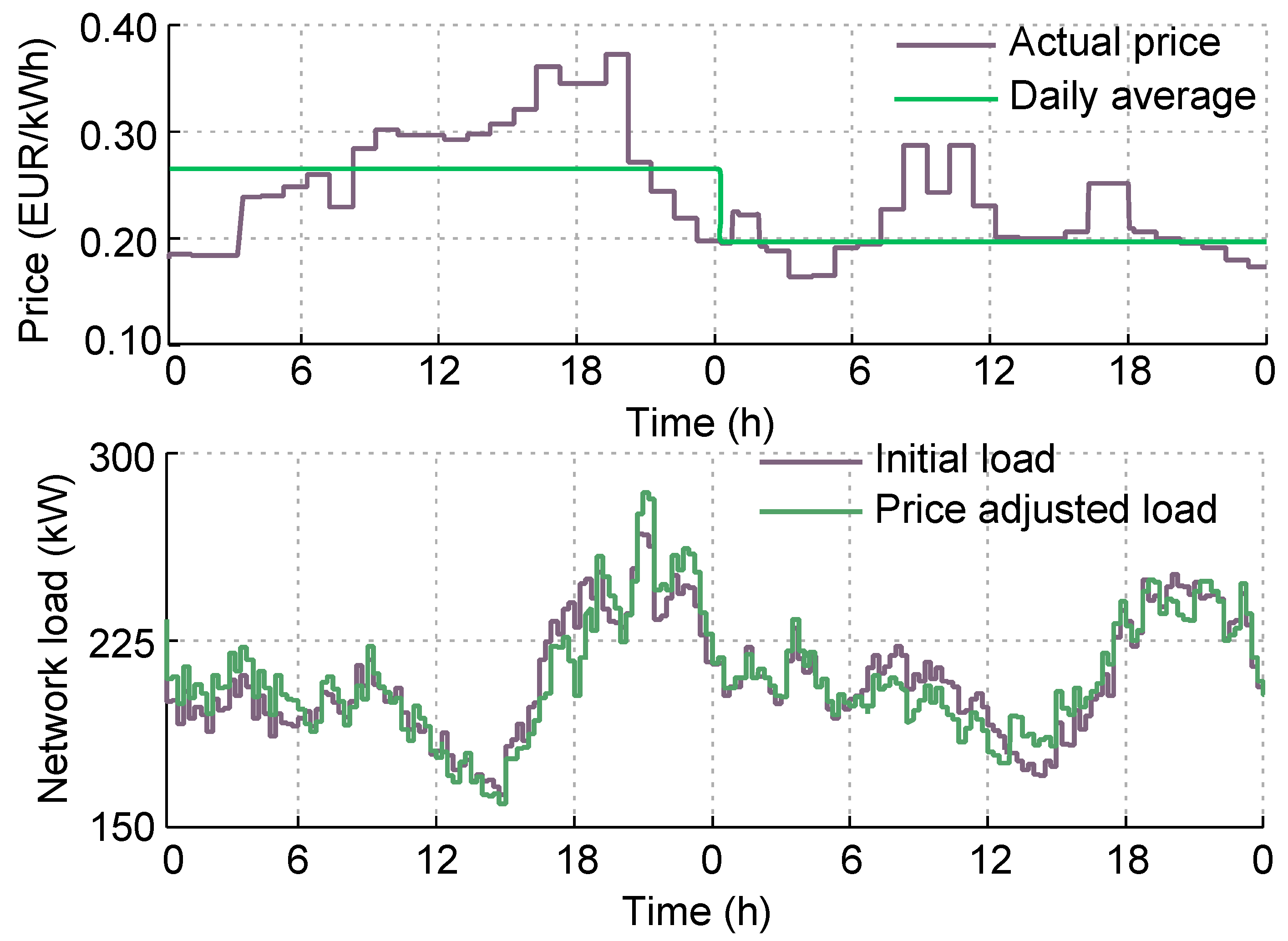
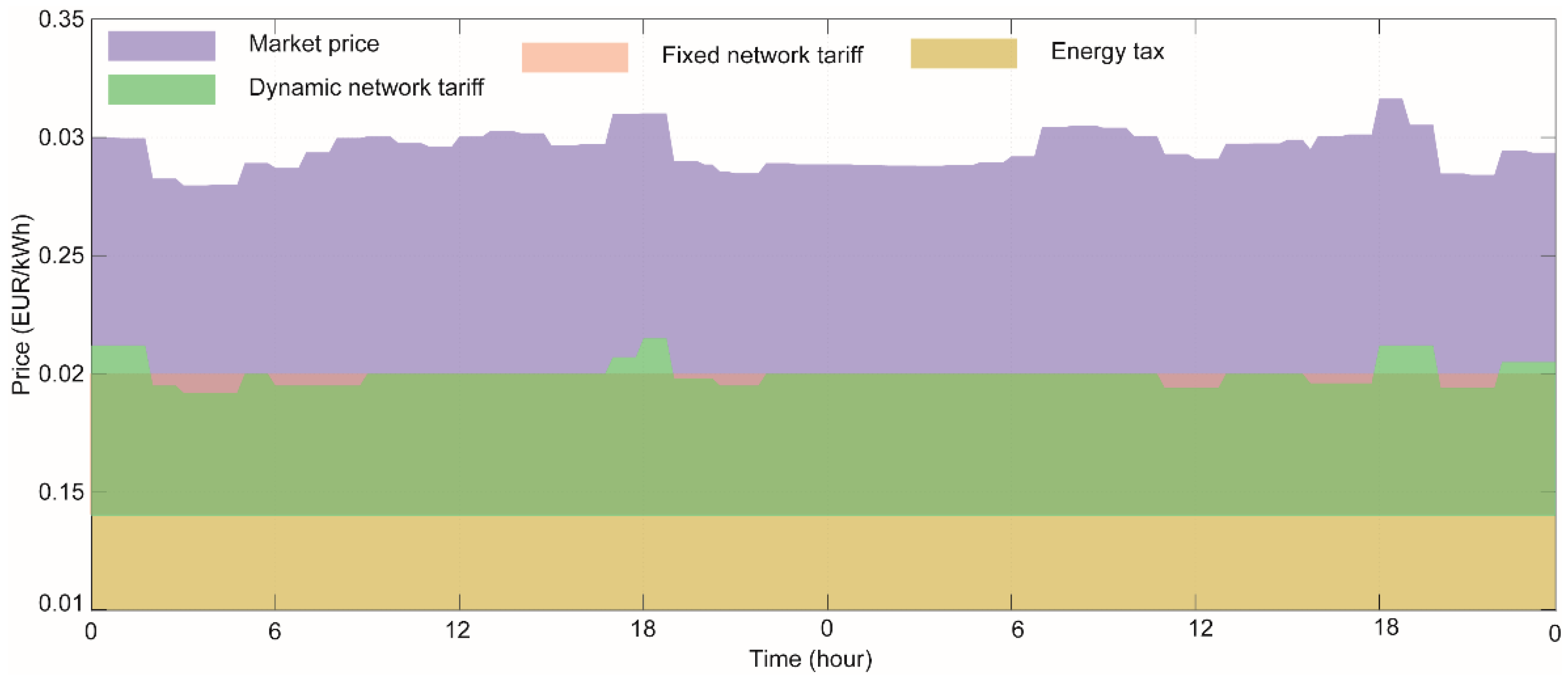
5.2. Effects of Dynamic Market Price
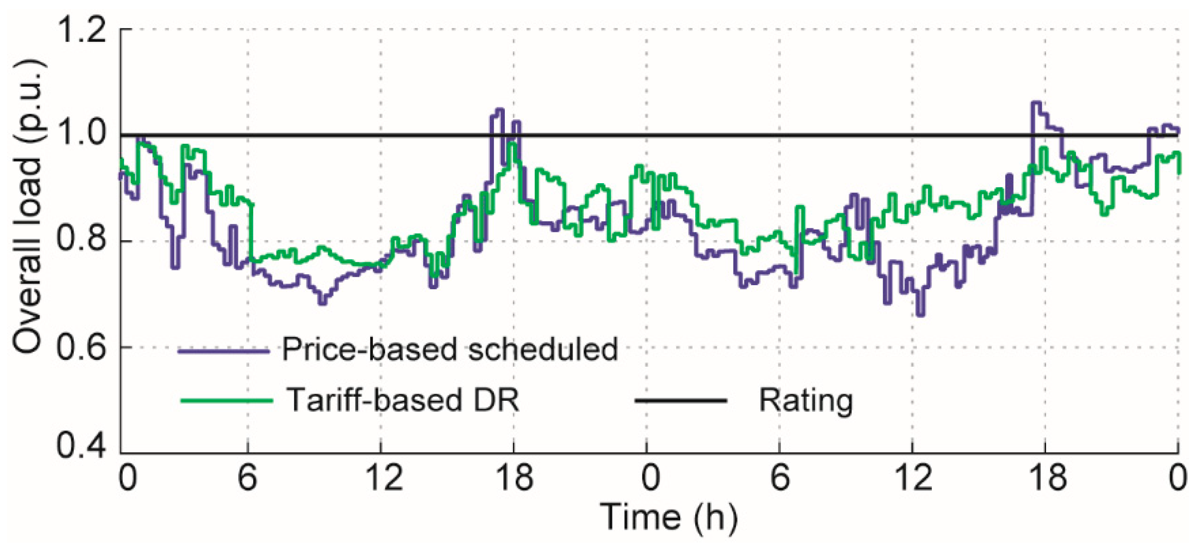
5.3. Dynamic Network Tariff for Peak Reduction
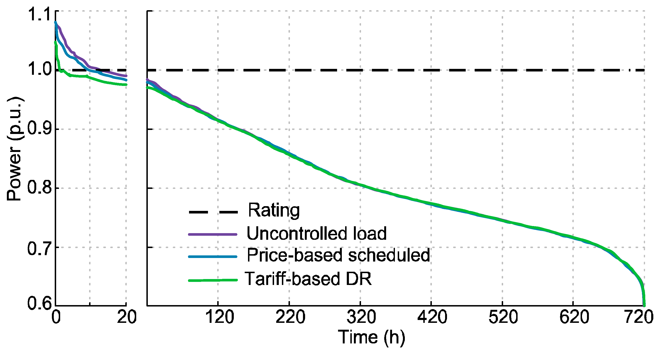
5.4. Monthly Assessment
6. Conclusions
Author Contributions
Funding
Conflicts of Interest
Nomenclature
| List of Abbreviations | |||
| CDF | Cumulative Distribution Function | KDE | Kernel Density Estimator |
| DA | Device Agent | LV | Low-voltage |
| DR | Demand Response | MAS | Multi-Agent Systems |
| DS | Dynamic Subsidy | MV | Medium-voltage |
| DSO | Distribution System Operator | PV | Photovoltaics |
| EPRI | Electric Power Research Institute | RES | Renewable Energy Sources |
| EV | Electric Vehicle | TA | Transformer Agent |
| HA | House Agent | TOC | Total Owning Cost |
| HP | Heat Pump | ||
| List of Symbols | |||
| Indices | hottest spot temperature | ||
| a | index of appliances | ambient temperature | |
| t | index of time steps | FAA | ageing acceleration factor |
| bf | index of buffer appliances | Feqv | equivalent factor |
| ts | index of time shifting appliances | Cag | ageing cost |
| D | index of day | Tlol | loss of life |
| s | index of scenarios | COL | overloading cost |
| Sets | Parameters | ||
| A | set of appliances | Nt | number of daily time steps |
| T | set of all time steps | duration of a time step in hour | |
| S | set of all scenarios | x | buffer time |
| Variables | lower limit of allowable time shift | ||
| p | electricity price | upper limit of allowable time shift | |
| P | active power | top oil temperature rise at rated load | |
| k | time shift of buffer appliances | hottest-spot temperature at rated load | |
| time shift of time shifting appliances | R | ratio of load loss to no-load loss | |
| K | load multiplex | Tinl | normal insulation life of transformer |
| top oil temperature rise | CP | purchase cost | |
| hottest spot temperature rise | CNL, CLL | cost of no-load loss and load loss | |
References
- Haque, A.N.M.M.; Nguyen, P.H.; Vo, T.H.; Bliek, F.W. Agent-based unified approach for thermal and voltage constraint management in LV distribution network. Electr. Power Syst. Res. 2017, 143, 462–473. [Google Scholar] [CrossRef]
- Haque, A.N.M.M.; Shafiullah, D.S.; Nguyen, P.H.; Bliek, F.W. Real-Time Congestion Management in Active Distribution Network based on Dynamic Thermal Overloading Cost. In Proceedings of the Power Systems Computation Conference (PSCC), Genoa, Italy, 20–24 June 2016; pp. 1–7. [Google Scholar]
- Veldman, E.; Verzijlbergh, R.A. Distribution Grid Impacts of Smart Electric Vehicle Charging from Different Perspectives. IEEE Trans. Smart Grid 2015, 6, 333–342. [Google Scholar] [CrossRef]
- Haque, A.N.M.M. Smart Congestion Management in Active Distribution Networks; Eindhoven University of Technology: Eindhoven, The Netherlands, 2017. [Google Scholar]
- Klaassen, E.A.M. Demand Response Benefits from a Power System Perspective; Eindhoven University of Technology: Eindhoven, The Netherlands, 2016. [Google Scholar]
- Haque, A.; Nijhuis, M.; Ye, G.; Nguyen, P.; Bliek, F.; Slootweg, J. Integrating Direct and Indirect Load Control for Congestion Management in LV Networks. IEEE Trans. Smart Grid 2017, 10, 741–751. [Google Scholar] [CrossRef]
- Li, Y.; Li, N. Mechanism design for reliability in demand response with uncertainty. In Proceedings of the American Control Conference, Seattle, WA, USA, 24–26 May 2017. [Google Scholar]
- Ma, H.; Parkes, D.C.; Robu, V. Generalizing demand response through reward bidding. In Proceedings of the International Joint Conference on Autonomous Agents and Multiagent Systems AAMAS, São Paulo, Brazil, 8–12 May 2017. [Google Scholar]
- Hu, J.; You, S.; Lind, M.; Østergaard, J. Coordinated charging of electric vehicles for congestion prevention in the distribution grid. IEEE Trans. Smart Grid 2014, 5, 703–711. [Google Scholar] [CrossRef]
- Liu, W.; Wu, Q.; Wen, F.; Ostergaard, J. Day-ahead congestion management in distribution systems through household demand response and distribution congestion prices. IEEE Trans. Smart Grid 2014, 5, 2739–2747. [Google Scholar] [CrossRef]
- Nguyen, P.H.; Kling, W.L.; Ribeiro, P.F. A game theory strategy to integrate distributed agent-based functions in smart grids. IEEE Trans. Smart Grid 2013, 4, 568–576. [Google Scholar] [CrossRef]
- Palensky, P.; Dietrich, D. Demand side management: Demand response, intelligent energy systems, and smart loads. IEEE Trans. Ind. Inf. 2011, 7, 381–388. [Google Scholar] [CrossRef]
- Ghazvini, M.A.F.; Lipari, G.; Pau, M.; Ponci, F.; Monti, A.; Soares, J.; Castro, R.; Vale, Z. Congestion management in active distribution networks through demand response implementation. Sustain. Energy Grids Netw. 2019, 17, 100185. [Google Scholar] [CrossRef]
- Garcia, T.S.; Shafie-Khah, M.; Osório, G.J.; Catalão, J.P.S. Optimal bidding strategy of responsive demands in a new decentralized market-based scheme. In Proceedings of the 17th IEEE International Conference on Environment and Electrical Engineering and 1st IEEE Industrial and Commercial Power Systems Europe, Milan, Italy, 6–9 June 2017. [Google Scholar]
- Chai, B.; Chen, J.; Yang, Z.; Zhang, Y. Demand response management with multiple utility companies: A two-level game approach. IEEE Trans. Smart Grid 2014, 5, 722–731. [Google Scholar] [CrossRef]
- Haque, A.N.M.M.; Nguyen, P.H.; Bliek, F.W.; Slootweg, J.G. Demand response for real-time congestion management incorporating dynamic thermal overloading cost. Sustain. Energy Grids Netw. 2017, 10, 65–74. [Google Scholar] [CrossRef]
- Nizami, M.S.H.; Haque, A.N.M.M.; Nguyen, P.H.; Bliek, F.W. HEMS as Network Support Tool: Facilitating Network Operator in Congestion Management and Overvoltage Mitigation. In Proceedings of the 16th International Conference on Environment and Electrical Engineering (EEEIC), Florence, Italy, 6–8 June 2016; pp. 1–6. [Google Scholar]
- Torbaghan, S.S.; Gibescu, M.; Rawn, B.G.; van der Meijden, M. A market-based transmission planning for HVDC grid—Case study of the North Sea. IEEE Trans. Power Syst. 2015, 30, 784–794. [Google Scholar] [CrossRef]
- Hu, J.; Saleem, A.; You, S.; Nordström, L.; Lind, M.; Østergaard, J. A multi-agent system for distribution grid congestion management with electric vehicles. Eng. Appl. Artif. Intell. 2015, 38, 45–58. [Google Scholar] [CrossRef]
- Zhang, C.; Ding, Y.; Østergaard, J.; Bindner, H.W.; Nordentoft, N.C.; Hansen, L.H.; Brath, P.; Cajar, P.D. A flex-market design for flexibility services through DERs. In Proceedings of the 4th IEEE/PES Innovative Smart Grid Technologies Europe, Copenhagen, Denmark, 6–9 October 2013. [Google Scholar]
- Huang, S.; Wu, Q.; Cheng, L.; Liu, Z.; Zhao, H. Uncertainty Management of Dynamic Tariff Method for Congestion Management in Distribution Networks. IEEE Trans. Power Syst. 2016, 3053, 1–12. [Google Scholar] [CrossRef]
- Huang, S.; Wu, Q. Dynamic Subsidy Method for Congestion Management in Distribution Networks. IEEE Trans. Smart Grid 2018, 9, 2140–2151. [Google Scholar] [CrossRef]
- Zhao, J.; Wang, Y.; Song, G.; Li, P.; Wang, C.; Wu, J. Congestion Management Method of Low-Voltage Active Distribution Networks Based on Distribution Locational Marginal Price. IEEE Access 2019, 7, 32240–32255. [Google Scholar] [CrossRef]
- Lampropoulos, I.; van den Broek, M.; van der Hoofd, E.; Hommes, K.; van Sark, W. A system perspective to the deployment of flexibility through aggregator companies in the Netherlands. Energy Policy 2018, 118, 534–551. [Google Scholar] [CrossRef]
- Biggar, D.; Reeves, A. Network Pricing for the Prosumer Future: Demand-Based Tariffs or Locational Marginal Pricing? In Future of Utilities–Utilities of the Future: How Technological Innovations in Distributed Energy Resources Will Reshape the Electric Power Sector; Academic Press: Cambridge, MA, USA, 2016. [Google Scholar]
- Torbaghan, S.S.; Blaauwbroek, N.; Nguyen, P.; Gibescu, M. Local market framework for exploiting flexibility from the end users. In Proceedings of the 2016 13th International Conference on the European Energy Market (EEM), Porto, Portugal, 6–9 June 2016; pp. 1–6. [Google Scholar] [CrossRef]
- Eid, C.; Codani, P.; Perez, Y.; Reneses, J.; Hakvoort, R. Managing electric flexibility from Distributed Energy Resources: A review for incentives, aggregation and market design. Renew. Sustain. Energy Rev. 2015, 64, 237–247. [Google Scholar] [CrossRef]
- Nwulu, N.I.; Xia, X. Optimal dispatch for a microgrid incorporating renewables and demand response. Renew. Energy 2017, 101, 16–28. [Google Scholar] [CrossRef]
- Pratt, B.A.; Krishnamurthy, D.; Ruth, M. Transactive Home Energy Management Systems. IEEE Electrif. Mag. 2016, 4, 8–14. [Google Scholar] [CrossRef]
- Minniti, S.; Haque, N.; Nguyen, P.; Pemen, G. Local markets for flexibility trading: Key stages and enablers. Energies 2018, 11, 3074. [Google Scholar] [CrossRef]
- Nijhuis, M.; Gibescu, M.; Cobben, J.F.G. Bottom-up Markov Chain Monte Carlo approach for scenario based residential load modelling with publicly available data. Energy Build. 2016, 112, 121–129. [Google Scholar] [CrossRef]
- Flexible Power Alliance Interface (FPAI). Available online: http://www.flexiblepower.org/downloads/ (accessed on 21 December 2019).
- Ni, F.; Nguyen, P.H.; Cobben, J.F.G. Basis-Adaptive Sparse Polynomial Chaos Expansion for Probabilistic Power Flow. IEEE Trans. Power Syst. 2017, 32, 694–704. [Google Scholar] [CrossRef]
- ABB. Distribution Transformer Handbook IEC/CENELEC Related Specifications ABB; ABB: Zurich, Switzerland, 2003. [Google Scholar]
- Downing, D.J.; McConnell, B.W.; Barnes, P.R.; Hadley, S.W.; van Dyke, J.W. Economic Analysis of Efficient Distribution Transformer Trends; Oak Ridge National Laboratory: Oak Ridge, TN, USA, 1998. [Google Scholar]
- Verzijlbergh, R.A.; Lukszo, Z.; Veldman, E.; Slootweg, J.G.; Ilic, M. Deriving electric vehicle charge profiles from driving statistics. In Proceedings of the IEEE Power & Energy Society General Meeting, Detroit, MI, USA, 24–28 July 2011; pp. 1–6. [Google Scholar]
- Verzijlbergh, R.A. The Power of Electric Vehicles; Delft University of Technology: Delft, The Netherlands, 2013. [Google Scholar]
- IEEE PES Distribution Test Feeder Working Group. Distribution Test Feeders. Available online: https://site.ieee.org/pes-testfeeders/resources/ (accessed on 21 December 2019).
- EPRI. OpenDSS, Distribution System Simulator. Available online: http://sourceforge.net/projects/electricdss (accessed on 26 June 2018).


| Performance Indicators | Uncontrolled Load | Price-Based Scheduling | Tariff-Based Dr |
|---|---|---|---|
| Maximum load (p.u.) | 1.07 | 1.07 | 1.05 |
| Duration of congestion (h) | 11.50 | 9.75 | 1.75 |
| Supplied energy (MWh) | 148.22 | 148.34 | 148.07 |
| Average domestic cost (EUR) | 43.88 | 41.23 | 42.02 |
© 2020 by the authors. Licensee MDPI, Basel, Switzerland. This article is an open access article distributed under the terms and conditions of the Creative Commons Attribution (CC BY) license (http://creativecommons.org/licenses/by/4.0/).
Share and Cite
Haque, N.; Tomar, A.; Nguyen, P.; Pemen, G. Dynamic Tariff for Day-Ahead Congestion Management in Agent-Based LV Distribution Networks. Energies 2020, 13, 318. https://doi.org/10.3390/en13020318
Haque N, Tomar A, Nguyen P, Pemen G. Dynamic Tariff for Day-Ahead Congestion Management in Agent-Based LV Distribution Networks. Energies. 2020; 13(2):318. https://doi.org/10.3390/en13020318
Chicago/Turabian StyleHaque, Niyam, Anuradha Tomar, Phuong Nguyen, and Guus Pemen. 2020. "Dynamic Tariff for Day-Ahead Congestion Management in Agent-Based LV Distribution Networks" Energies 13, no. 2: 318. https://doi.org/10.3390/en13020318
APA StyleHaque, N., Tomar, A., Nguyen, P., & Pemen, G. (2020). Dynamic Tariff for Day-Ahead Congestion Management in Agent-Based LV Distribution Networks. Energies, 13(2), 318. https://doi.org/10.3390/en13020318