Pressure-Transient Performances of Fractured Horizontal Wells in the Compartmentalized Heterogeneous Unconventional Reservoirs

Abstract

In order to investigate pressure performance of multiple fractured horizontal wells (MFHWs) penetrating heterogeneous unconventional reservoir and avoid the high computational cost of numerical simulation, a semi-analytical model for MFHWs combining Green function solution and boundary element method has been obtained, where the reservoir is divided into different homogeneous substructures and coupled at interface boundaries by plane source function in a closed rectangular parallelepiped. Hydraulic fractures are assumed uniform flux and dual porosity model is used for natural fractures system. Then the model is validated by compared with analytical solution of MFHWs in a homogeneous reservoir and trilinear flow model, which shows that this model can achieve high accuracy even with a small interface discretization number, and it can consider the radial flow around each hydraulic fractures. Finally, the pressure responses with heterogeneous parameters of reservoirs are discussed including heterogeneous permeability, non-uniform block-length and fracture half-length distribution as well as dual porosity parameters like elastic storage ratio and crossflow ratio.

1. Introduction

With the rapid development of unconventional reservoirs, the horizontal well intercepted by hydraulic fractures has become the main technology [1,2], which can significantly increase contact areas between fractures and formation zone. Thus, the transient performances of Multiple Fractured Horizontal Wells (MFHWs) have attracted more and more scholars’ attention. There have been extensive studies [3,4,5] on the MFHWs of unconventional reservoir, which generally can be classified into analytical model, numerical model and semi-analytical model.

To consider the effect of formation heterogeneity, one of the most common analytical models is the trilinear flow model with three different flow areas of outer region, inner region and hydraulic fracture, which is proposed by Brown [6]. To describe the hydraulic fractures surrounding by the stimulated area, Stalgorova [7,8] subdivided the trilinear flow regions into five flow regions model. Guo [9] extended the flow area into seven parts including various fracture distribution along the horizontal wellbore. Later, on account of the fractal nature of fractured media, the new formulations are implemented in the trilinear flow model using fractal theory [3,10,11]. The fundamental petro-physical characteristic of unconventional reservoirs is considered, but all multi-linear models are based on two critical assumptions. One assumption is that fluid flow obeys linear flow in all regions. As a result, some other flow regimes are ignored such as first radial flow around hydraulic fractures and later elliptical flow [12]. The other assumption is that the formation properties around each fracture are assumed to be the same, and the interference between different fractures is not investigated. However, Zawilla [13] and Liu [14] indicated that heterogeneous properties are commonly existed in the unconventional reservoir formation and different fracturing stages.

The numerical simulation is an effective method to model the flow performance of MFHWs, which can deal with the formation heterogeneity easily. Especially, Discrete Fracture Model (DFM) [4,15,16] is used for complex fracture network with high computational costs, which accounts the effects of individual fractures explicitly. In order to avoid lots of meshing of unstructured grid around each fracture, Embedded Discrete Fracture Method (EDFM) is proposed [17] by orthogonal coarse grid instead of fine small unstructured grid, but the transient performance of MFHWs needs detailed pressure solution by small space scale and time scale.

Since Gringarten [18] (1973) introduced the source/Green’s function solution into the fluid flow in porous media, this semi-analytical method has greatly expanded our ability to solve different well problems. The transient performances of MFHWs are calculated by many authors [19,20]. Then, Ozkan and Raghavan [21,22] (1991) used Laplace transformation into the source function, which can easily extend to the naturally fractured media and variable rate production condition. After that, relevant transient solutions of MFHWs are obtained [23,24,25]. Most of their works focus on the different fracture distributions and different reservoir types, while reservoir heterogeneity is less studied. To consider the Stimulated Reservoir Volume (SRV) in the unconventional reservoir, a composite model [5,26,27] is built by deriving point source solution from circular composite reservoir. However, the structure of MFHWs in composite circular reservoirs cannot match the linear flow around the SRV area and the reservoir heterogeneity around each fracture is not considered either.

For the heterogeneous reservoirs, Kikani [28] (1993) modeled the pressure performance of different sectional homogeneous reservoir by BEM (boundary element method). Idorenyin [29] (2016) considered the arbitrary-shaped composite reservoirs by extending Kikani’s model. Based on the element boundary method and Green’s function, Medeiros [30] (2010) presented a semi-analytical model for the pressure transient analysis of horizontal wells in heterogeneous reservoirs. Based on the fact that the main contribution for hydrocarbon flow rate of MFHWs is the SRV area [31], so this paper is to build a semi-analytical model for MFHWs in heterogeneous stimulated reservoir volume of naturally fractured media. To avoid fine grid of numerical reservoir simulator around fractures and wells, the plane source functions in the closed domain and boundary element method are applied, where stimulated reservoir volume is divided into compartmentalized heterogeneous blocks. In addition, the result is verified with other analytical methods. Finally, heterogeneous effects on pressure and production performance are presented.

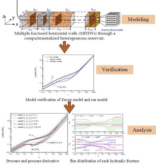
2. Modeling of MFHWs

Firstly, we will present basic the physical model and assumption for hydraulic fractures and stimulated reservoir volume (SRV). Then, the Green’s function formulation of the pressure-transient solution for a locally homogeneous reservoir substructure will be given with inner and outer boundaries.

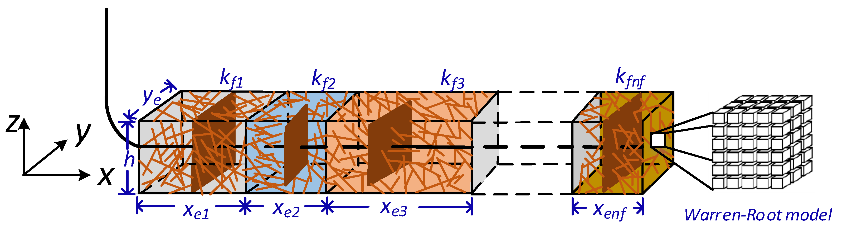
2.1. Physical Model and Assumptions

A Multiple fractured horizontal well passing through a heterogeneous reservoir with different properties is shown in Figure 1, where each block is the subsections of the reservoir characterized by uniform average properties. Except for the interfaces between the blocks, other boundaries of the blocks are assumed to be impermeable. The basic assumptions of the model are as follows:

(1)

The reservoir is heterogeneous along the horizontal wellbore with n_f blocks of different length x_ei (i = 1, 2, 3, …, n_f), and there is one hydraulic fracture distributed in each block. The thickness of the stimulated reservoir volume is uniform h and width is y_e. The initial pressure is assumed p_i.

(2)

The artificial hydraulic fractures are vertical to the horizontal wellbore, with fracture half-length L_fi, fracture height h_fi, (i = 1, 2, 3, …, n_f), and uniform flux distribution assumed in each hydraulic fracture.

(3)

Each block of unconventional reservoir was established by Warren and Root’s (1963) dual porosity model, where natural fractures and matrix follow the Darcy’s flow model. For each blocks, different natural fracture permeability k_fi, crossflow coefficient λ_i, and elastic storage ratio ω_i (i = 1, 2, 3, …, n_f) can be defined.

(4)

The fluid assumed slightly compressible with constant viscosity and compressibility.

(5)

Gravity and capillary effect are negligible.

2.2. Pressure Solution for a Reservoir Substructure

Based on the Green’s function, the pressure transient solution of dimensionless space and time in porous media can be written as follows [18,31,32], where the domain boundary is divided into the inner and outer boundaries, represented by B_wD, and B_eD, respectively:

$$\begin{array}{cc}\Delta p\left(M_D,t_D\right)=& -{{\displaystyle \int }}_0^{t_D}{{\displaystyle \int }}_{{\mathrm{B}}_{\mathrm{wD}}}{\left[G\left(M_D,M_D^{\prime },t_D-\tau \right)\frac{\partial p\left(M_D^{\prime },\tau \right)}{\partial n_{B_{wD}}}-p\left(M_D^{\prime },\tau \right)\frac{\partial G\left(M_D,M_D^{\prime },t_D-\tau \right)}{\partial n_{B_{wD}}}\right]}_{M_D^{\prime }\in B_{wD}}d{M}_D^{\prime }d\tau \\ & -{{\displaystyle \int }}_0^{t_D}{{\displaystyle \int }}_{{\mathrm{B}}_{\mathrm{eD}}}{\left[G\left(M_D,M_D^{\prime },t_D-\tau \right)\frac{\partial p\left(M_D^{\prime },\tau \right)}{\partial n_{B_{eD}}}-p\left(M_D^{\prime },\tau \right)\frac{\partial G\left(M_D,M_D^{\prime },t_D-\tau \right)}{\partial n_{B_{eD}}}\right]}_{M_D^{\prime }\in B_{eD}}d{M}_D^{\prime }d\tau \end{array}$$

(1)

where $\Delta p\left(M_D,t_D\right)$ is the pressure drop, $G\left(M_D,M_D^{\prime },t_D-\tau \right)$ is the Green’s function, $p\left(M_D^{\prime },\tau \right)$ is the pressure. The $B_{wD}$ corresponds to well surface and $B_{\mathrm{e}D}$ is the outer surface of the dimensionless domain, the points $M_D$ and $M_D^{\prime }$ represent the observation and source locations in dimensionless space, respectively, and t_D is dimensionless time, and defined as:

$$t_D=\frac{k}{\varphi C_t\mu {\ell }^2}t$$

(2)

where, $\mu$ is the fluid viscosity, k is the permeability, $\ell$ is the characteristic reference length, $C_t$ is the total compressibility, $\varphi$ is the porosity and t is time.

Then, the homogeneous Neumann boundary condition is used to eliminate partial derivative of Green function. The point flux term is obtained by Darcy’s law to represent the normal pressure derivatives on the boundary surfaces. Therefore, we can rewrite Equation (1) as follows:

$$\begin{gathered} \Delta p\left(M_D,t_D\right)=\underset{0}{\overset{t_D}{{\displaystyle \int }}}\underset{{\mathrm{B}}_{\mathrm{wD}}}{{\displaystyle \int }}{\tilde{q}}_w\left(M_D^{\prime },\tau \right)G\left(M_D,M_D^{\prime },t_D-\tau \right)d{M}_D^{\prime }d\tau \\ \hspace{1em}\hspace{1em}\hspace{1em}\hspace{1em}\hspace{1em}+\underset{0}{\overset{t_D}{{\displaystyle \int }}}\underset{{\mathrm{B}}_{\mathrm{eD}}}{{\displaystyle \int }}{\tilde{q}}_e\left(M_D^{\prime },\tau \right)G\left(M_D,M_D^{\prime },t_D-\tau \right)d{M}_D^{\prime }d\tau \end{gathered}$$

(3)

where,${\tilde{q}}_w\left(M_D^{\prime },\tau \right)$, ${\tilde{q}}_e\left(M_D^{\prime },\tau \right)$ are the point flux of well surface and outer surface, respectively. We divide the inner and outer boundary surface into n and m segments of uniform flux, and the source function are defined as

$$B_{wD}={\displaystyle \sum }_{j=1}^n{B}_{wDj}\begin{array}{ccc}& & j=1,2,3,\cdots ,n\end{array}$$

(4)

$$B_{eD}={\displaystyle \sum }_{k=1}^m{B}_{eDk}\begin{array}{ccc}& & k=1,2,3,\cdots ,m\end{array}$$

(5)

$$S_{\alpha }\left(M_D,t_D\right)=\underset{B_{\alpha }}{{\displaystyle \int }}G\left(M_D,M_D^{\prime },t_D-\tau \right)d{M}_D^{\prime }\begin{array}{cc}& \mathrm{for}\begin{array}{cc} \alpha =wDj \begin{array}{cc}\mathrm{or} \begin{array}{cc}eDk& \end{array}& \end{array}& \end{array}\end{array}$$

(6)

Therefore, the Equation (3) can be rewritten as follows:

$$\begin{gathered} \Delta p\left(M_D,t_D\right)={\displaystyle \sum }_{j=1}^n\underset{0}{\overset{t_D}{{\displaystyle \int }}}{\tilde{q}}_{wj}\left(\tau \right)S_{wDj}\left(M_D,t_D-\tau \right)d\tau \\ \hspace{1em}\hspace{1em}\hspace{1em}\hspace{1em}\hspace{1em}+{\displaystyle \sum }_{k=1}^m\underset{0}{\overset{t_D}{{\displaystyle \int }}}{\tilde{q}}_{ek}\left(\tau \right)S_{eDk}\left(M_D,t_D-\tau \right)d\tau \end{gathered}$$

(7)

Ozkan and Raghavan [21] applied the Laplace transformation into Equation (7), the variable flow rate condition and naturally fractured media can be easily implemented by Green’s function. Convert the convolution integrals into algebraic expressions. Then, Equation (7) can be rewritten as

$$\overline{\Delta p}\left(M_D,s\right)={\displaystyle \sum }_{j=1}^{n}s\times {\overline{\tilde{q}}}_{wj}\left(s\right){\overline{S}}_{wDj}\left(M_D,s\right)+{\displaystyle \sum }_{k=1}^{m}s\times {\overline{\tilde{q}}}_{ek}\left(s\right){\overline{S}}_{eDk}\left(M_D,s\right)$$

(8)

The function with bar signs in Equation (8) indicates their function in Laplace transforms with respect to the time t_D, and s is the Laplace-transform variable.

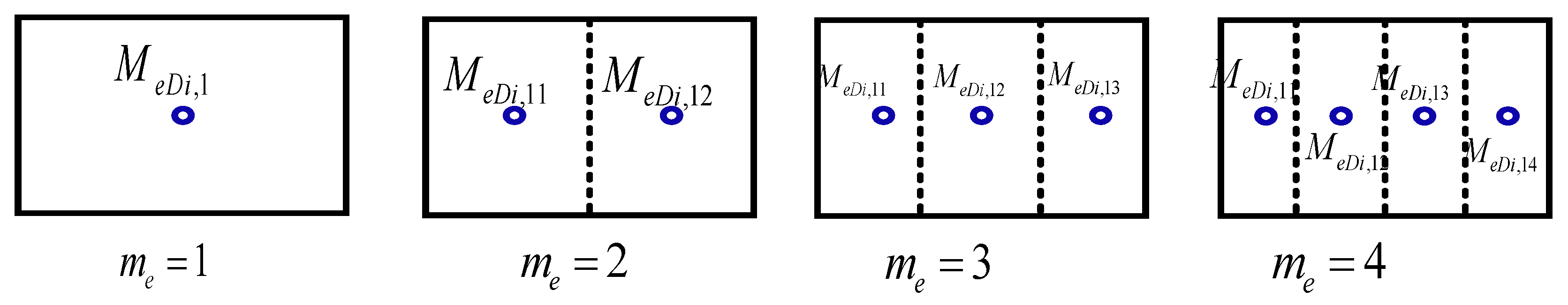
2.3. Source Functions for the Inner and Outer Boundaries

To obtain the transient pressure solution of fractured horizontal well in a rectangular parallelepiped, the source functions of inner and outer boundaries are evaluated by the Green’s function. For the partial and full penetration of the hydraulic fractures in the reservoir, 3D plane source and 2D line source should be considered.

Corresponding to the point source in the rectangular parallelepiped, the Green’s function in dual porous media can be expressed as [21]

$$\begin{array}{c}\overline{G}\left(M_D,M_D^{\prime },s\right)=\frac{\mu }{2k_f\ell y_{eD}{h}_D}\{\frac{\mathrm{ch}\left(\sqrt{u}{x}_{D1}\right)+\mathrm{ch}\left(\sqrt{u}{x}_{D2}\right)}{\sqrt{u}\mathrm{sh}\left(\sqrt{u}{x}_{eD}\right)}\\ \hspace{1em}\hspace{1em}\hspace{1em}+2{\displaystyle {\displaystyle \sum }_{k=1}^{\infty }}\cos k\pi \frac{y_D}{y_{eD}}\cos k\pi \frac{y_D^{\prime }}{y_{eD}}\frac{\mathrm{ch}\left({\epsilon }_k{x}_{D1}\right)+\mathrm{ch}\left({\epsilon }_k{x}_{D2}\right)}{{\epsilon }_k\mathrm{sh}\left({\epsilon }_k{x}_{eD}\right)}\\ \hspace{1em}\hspace{1em}\hspace{1em}+2{\displaystyle {\displaystyle \sum }_{n=1}^{\infty }}\cos n\pi \frac{z_D}{h_D}\cos n\pi \frac{z_{wD}}{h_D}[\frac{\mathrm{ch}\left({\epsilon }_n{x}_{D1}\right)+\mathrm{ch}\left({\epsilon }_n{x}_{D2}\right)}{{\epsilon }_n\mathrm{sh}\left({\epsilon }_n{x}_{eD}\right)}\\ \hspace{1em}\hspace{1em}\hspace{1em}+2{\displaystyle {\displaystyle \sum }_{k=1}^{\infty }}\cos k\pi \frac{y_D}{y_{eD}}\cos k\pi \frac{y_D^{\prime }}{y_{eD}}\frac{\mathrm{ch}{\epsilon }_{k,n}{x}_{D1}+\mathrm{ch}{\epsilon }_{k,n}{x}_{D2}}{{\epsilon }_{k,n}\mathrm{sh}\left({\epsilon }_{k,n}{x}_{eD}\right)}]\}\end{array}$$

(9)

In Equation (9), we have defined$M_D=\left(x_D,y_D,z_D\right)$,$M_D^{\prime }=\left(x_D^{\prime },y_D^{\prime },z_D^{\prime }\right)$,$x_{\mathrm{eD}}=\frac{x_e}{\ell }$,$y_{\mathrm{eD}}=\frac{y_e}{\ell }{h}_{\mathrm{D}}=\frac{h}{\ell }$, $x_{\mathrm{D}1}=x_{eD}-\left|x_D-x_{\mathrm{D}}^{\prime }\right|$,$x_{\mathrm{D}2}=x_{eD}-\left|x_D+x_{\mathrm{D}}^{\prime }\right|$,${\epsilon }_n=\sqrt{u+{\left(n\pi /h_D\right)}^2}$,${\epsilon }_k=\sqrt{u+{\left(k\pi /y_{eD}\right)}^2}$,${\epsilon }_{k,n}=\sqrt{u+{\left(k\pi /y_{eD}\right)}^2+{\left(n\pi /h_D\right)}^2}$ and $u=sf\left(s\right)$, $f\left(s\right)=\frac{s\omega \left(1-\omega \right)+\lambda }{\lambda +s\left(1-\omega \right)}$ for naturally fractured reservoir.

The inner and outer boundaries consist of the planar surfaces in the rectangular parallelepiped, which represented hydraulic fractures and boundary planes. The source function for a plane is perpendicular to the x-axis, so a planar source in the y-z plane can be calculated by integration of Equation (9) (shown in Figure 2)

$$\begin{array}{c}\overline{S}\left(M_D,s\right)={{\displaystyle \int }}_{-h_{wD}/2}^{h_{wD}/2}{{\displaystyle \int }}_{-L_{fD}}^{L_{fD}}\overline{G}\left(M_D,M_D^{\prime },s\right)d{y}_D^{\prime }d{z}_D^{\prime }\\ =\frac{\mu L_{fD}{h}_{wD}}{kh{\mathrm{y}}_{eD}}\{\frac{\mathrm{ch}\left(\sqrt{u}{x}_{D1}\right)-\mathrm{ch}\left(\sqrt{u}{x}_{D2}\right)}{\sqrt{u}sh\left(\sqrt{u}{x}_{eD}\right)}+\frac{2y_{eD}}{\pi L_{fD}}{\displaystyle \sum }_{k=1}^{\infty }\frac{1}{k}\cos \left(k\pi \frac{y_D}{y_{eD}}\right)\cos \left(k\pi \frac{y_{wD}}{y_{eD}}\right)\sin \left(k\pi \frac{L_{fD}}{y_{eD}}\right)\\ \frac{\mathrm{ch}{\epsilon }_k{x}_{D1}-\mathrm{ch}{\epsilon }_k{x}_{D2}}{{\epsilon }_{k}sh{\epsilon }_k{x}_{eD}}\}+\frac{\mu }{\pi kh}\times \frac{4h_D{L}_{fD}}{{\mathrm{y}}_{eD}s}{\displaystyle \sum }_{n=1}^{\infty }\frac{1}{n}\cos \left(n\pi \frac{z_D}{h_D}\right)\sin \left(n\pi \frac{z_{wD}}{h_D}\right)\cos \left(n\pi \frac{h_{wD}}{2h_D}\right)\\ \{\frac{\mathrm{ch}{\epsilon }_n{x}_{D1}-\mathrm{ch}{\epsilon }_n{x}_{D2}}{{\epsilon }_{n}sh{\epsilon }_n{x}_{eD}}+\frac{2y_{eD}}{\pi L_{fD}}{\displaystyle \sum }_{k=1}^{\infty }\frac{1}{k}\sin \left(k\pi \frac{y_D}{y_{eD}}\right)\cos \left(k\pi \frac{y_{wD}}{y_{eD}}\right)\sin \left(k\pi \frac{L_{fD}}{y_{eD}}\right)\frac{\mathrm{ch}{\epsilon }_{n,k}{x}_{D1}-\mathrm{ch}{\epsilon }_{n,k}{x}_{D2}}{{\epsilon }_{n,k}sh{\epsilon }_{n,k}{x}_{eD}}\}\end{array}$$

(10)

When the reservoir is fully penetrated by hydraulic fractures, the boundary surface is at full penetration, namely $h_{wD}=h_D$; thus, Equation (10) can simplify to (the second item of Equation (10) is equal to 0)

$$\begin{array}{c}\overline{S}\left(M_D,s\right)=\frac{\mu L_{fD}{h}_{wD}}{kh{\mathrm{y}}_{eD}}\{\frac{\mathrm{ch}\left(\sqrt{u}{x}_{D1}\right)-\mathrm{ch}\left(\sqrt{u}{x}_{D2}\right)}{\sqrt{u}sh\left(\sqrt{u}{x}_{eD}\right)}+\frac{2y_{eD}}{\pi L_{fD}}{\displaystyle \sum }_{k=1}^{\infty }\frac{1}{k}\cos \left(k\pi \frac{y_D}{y_{eD}}\right)\cos \left(k\pi \frac{y_{wD}}{y_{eD}}\right)\sin \left(k\pi \frac{L_{fD}}{y_{eD}}\right)\\ \frac{\mathrm{ch}{\epsilon }_k{x}_{D1}-\mathrm{ch}{\epsilon }_k{x}_{D2}}{{\epsilon }_{k}sh{\epsilon }_k{x}_{eD}}\}\end{array}$$

(11)

3. Solution of Coupling Multiple Blocks

To obtain the pressure drop solution of MFHW in multiple reservoir blocks, we will demonstrate the coupling process of n_f rectangular reservoir blocks in series in the x direction as shown in Figure 1. Then, the pressure solution process of the linear system of equations is presented.

The fractured horizontal well extends through a heterogeneous reservoir with rectangular parallelepiped blocks. All block boundary surfaces are assumed to be impermeable, except for the interface between different blocks. We will assume that the hydraulic fractures are uniform flux distribution. For the infinite conductivity condition, the pressure response can be achieved by subdividing each fracture or assumed by 0.732 point pressure of fracture, and finite conductivity fractures can be obtained by incorporating pressure drop with hydraulic fractures [24]. Here, each hydraulic fracture as one segment represents inner boundary of each block, while boundary surfaces are discretized into m_e segments. From Equation (8), the pressure drop at the center of the ith fracture can be given by

$$\begin{array}{c}\overline{\Delta p}\left(M_{Dwi},s\right)\hfill \\ =\{\begin{array}{c}{\overline{\tilde{q}}}_{w1}\left(s\right){\overline{S}}_{wD1}\left(M_{Dw1},s\right)+{\displaystyle {\displaystyle \sum }_{k=1}^{m_e}}{\overline{\tilde{q}}}_{e1,2k}\left(s\right){\overline{S}}_{eD1,2k}\left(M_{Dw1},s\right)i=1\\ {\overline{\tilde{q}}}_{wi}\left(s\right){\overline{S}}_{wDi}\left(M_{Dwi},s\right)+{\displaystyle {\displaystyle \sum }_{k=1}^{m_e}}{\overline{\tilde{q}}}_{ei,1k}\left(s\right){\overline{S}}_{eDi,1k}\left(M_{Dwi},s\right)+{\displaystyle {\displaystyle \sum }_{k=1}^{m_e}}{\overline{\tilde{q}}}_{ei,2k}\left(s\right){\overline{S}}_{eDi,2k}\left(M_{Dwi},s\right)i=2,3,\dots ,n_f-1\\ {\overline{\tilde{q}}}_{w{n}_f}\left(s\right){\overline{S}}_{wD{n}_f}\left(M_{Dw{n}_f},s\right)+{\displaystyle {\displaystyle \sum }_{k=1}^{m_e}}{\overline{\tilde{q}}}_{e{n}_f,1k}\left(s\right){\overline{S}}_{eD{n}_f,1k}\left(M_{Dw{n}_f},s\right)i=n_f\end{array}\hfill \end{array}$$

(12)

where $M_{Dwi}$ indicate the center point of ith fracture, so ${\overline{\tilde{q}}}_{wi}$ is the point $M_{Dwi}$ flux, ${\overline{S}}_{eDi,1k}\left(M_{Dwi},s\right)$ and ${\overline{S}}_{eDi,2k}\left(M_{Dwi},s\right)$ are the source function of left and right surface at point $M_{Dwi}$ in ith block, respectively.

The pressure drop at the kth segment of two interfaces of ith block, where the left face marked 1, and right face marked 2, can be given by

$$\begin{array}{c}\overline{\Delta p}\left(M_{Dei,1k},s\right)\hfill \\ =\{\begin{array}{c}{\overline{\tilde{q}}}_{wi}\left(s\right){\overline{S}}_{wDi}\left(M_{Dei,1k},s\right)+{\displaystyle {\displaystyle \sum }_{k=1}^{m_e}}{\overline{\tilde{q}}}_{ei,1k}\left(s\right){\overline{S}}_{eDi,1k}\left(M_{Dei,1k},s\right)+\\ +{\displaystyle {\displaystyle \sum }_{k=1}^{m_e}}{\overline{\tilde{q}}}_{ei,2k}\left(s\right){\overline{S}}_{eDi,2k}\left(M_{Dei,1k},s\right), i=2,3,\cdots ,n_f-1\\ {\overline{\tilde{q}}}_{w{n}_f}\left(s\right){\overline{S}}_{wD{n}_f}\left(M_{De{n}_f,1k},s\right)+{\displaystyle {\displaystyle \sum }_{k=1}^{m_e}}{\overline{\tilde{q}}}_{e{n}_f,1k}\left(s\right){\overline{S}}_{eD{n}_f,1k}\left(M_{De{n}_f,1k},s\right),\begin{array}{ccc}& & i=n_f\end{array}\end{array}\hfill \end{array}$$

(13)

$$\begin{array}{c}\overline{\Delta p}\left(M_{Dei,2k},s\right)\hfill \\ =\{\begin{array}{c}{\overline{\tilde{q}}}_{w1}\left(s\right){\overline{S}}_{wD1}\left(M_{De1,2k},s\right)+{\displaystyle {\displaystyle \sum }_{k=1}^{m_e}}{\overline{\tilde{q}}}_{e1,2k}\left(s\right){\overline{S}}_{eD1,2k}\left(M_{De1,2k},s\right), i=1\\ {\overline{\tilde{q}}}_{wi}\left(s\right){\overline{S}}_{wDi}\left(M_{Dei,2k},s\right)+{\displaystyle {\displaystyle \sum }_{k=1}^{m_e}}{\overline{\tilde{q}}}_{ei,1k}\left(s\right){\overline{S}}_{eDi,1k}\left(M_{Dei,2k},s\right)+\\ +{\displaystyle {\displaystyle \sum }_{k=1}^{m_e}}{\overline{\tilde{q}}}_{ei,2k}\left(s\right){\overline{S}}_{eDi,2k}\left(M_{Dei,2k},s\right), i=2,3,\cdots ,n_f-1 \end{array}\hfill \end{array}$$

(14)

where $k=1, 2, 3,\dots .,m_e$, $M_{Dei,1k}$, $M_{Dei,2k}$ indicate the center point of kth segment of left and right surface in ith block, so ${\overline{\tilde{q}}}_{ei,1k}{\overline{\tilde{q}}}_{ei,2k}$ is the according flux of point $M_{Dei,1k}$ and$M_{Dei,2k}$, respectively.

Except the first and last block of SRV, each block has 1 + 2m_e points with unknown parameters of pressure and flux, therefore there are $\left(1+2m_e\right)\times 2\times n_f-4m_e$ unknown. Based on Equations (12)–(14), we yield $n_f+2\left(n_f-1\right)\times m_e$ linear equations. In order to get the same number of equations as the unknowns, the pressure and flux continuity condition can be applied.

(1)

Continuity conditions of pressure and flux at the interface

The pressure drop of the same interface should be equal for each segment k of different blocks, and the flux of interfaces should be continuous, so we have

$$\{\begin{array}{cc}\begin{array}{c}\overline{\Delta p}\left(M_{Dei,2\mathrm{k}},s\right)=\overline{\Delta p}\left(M_{Dei+1,1k},s\right)\\ \overline{\tilde{q}}\left(M_{Dei,2\mathrm{k}},s\right)=-\overline{\tilde{q}}\left(M_{Dei+1,1k},s\right)\end{array}& \begin{array}{cc}& i=1,2,3,\dots ,n_f-1\end{array}\begin{array}{cc}& \end{array}k=1,2,3,\dots ,m_e\end{array}$$

(15)

(2)

Horizontal wellbore conditions

Assuming that the horizontal wellbore is infinite conductivity, the pressure drop of each fracture mid-point $M_{Dwi}$ should be equal to the pressure drop of horizontal wellbore $\overline{\Delta p}\left(M_{Dw},s\right)$, so we can have n_f − 1 additional equations

$$\overline{\Delta p}\left(M_{Dwi},s\right)=\overline{\Delta p}\left(M_{Dw},s\right)\begin{array}{cc}& i=1,2,3,\dots ,n_f\end{array}$$

(16)

Moreover, the sum of the fluxes from all hydraulic fractures should be equal to the total production rate q_total.

$${\displaystyle \sum }_{i=1}^{n_f}{\overline{\tilde{q}}}_{wi}2L_{fi}{h}_{ei}=q_{total}/s$$

(17)

The linear system defined by Equations (12)–(17) has $\left(1+2m_e\right)\times 2\times n_f-4m_e$ equations for $\left(1+2m_e\right)\times 2\times n_f-4m_e$ unknowns, which can be written in the matrix-vector form AX = B. Here, take a multiple fractured horizontal well with n_f fractures and boundary segment m_e = 1; for example, the components of coefficient matrix A is

$$A={\left[\begin{array}{ccccccccc}s\times {\overline{S}}_{w1}^{w1}& s\times {\overline{S}}_{e1,2}^{w1}& 0& 0& 0& \cdots & 0& 0& -1\\ s\times {\overline{S}}_{w1}^{e1,2}& s\times \left({\overline{S}}_{e1,2}^{e1,2}+{\overline{S}}_{e2,1}^{e2,1}\right)& -s\times {\overline{S}}_{w2}^{e2,1}& -s\times {\overline{S}}_{e2,2}^{e2,1}& 0& \cdots & 0& 0& 0\\ 0& -s\times {\overline{S}}_{e2,1}^{w2}& s\times {\overline{S}}_{w2}^{w2}& s\times {\overline{S}}_{e2,2}^{w2}& 0& \cdots & 0& 0& -1\\ 0& -s\times {\overline{S}}_{e2,1}^{e2,2}& -s\times {\overline{S}}_{w2}^{e2,2}& s\times \left({\overline{S}}_{e2,2}^{e2,2}+{\overline{S}}_{e3,1}^{e3,1}\right)& -s\times {\overline{S}}_{w3}^{e3,1}& \cdots & 0& 0& 0\\ 0& 0& 0& -s\times {\overline{S}}_{e3,1}^{w3}& -s\times {\overline{S}}_{w3}^{w3}& \cdots & 0& 0& -1\\ ⋮& ⋮& ⋮& ⋮& ⋮& \ddots & ⋮& ⋮& ⋮\\ 0& 0& 0& 0& 0& \cdots & -s\times {\overline{S}}_{e{n}_f,1}^{w{n}_f}& s\times {\overline{S}}_{w{n}_f}^{w{n}_f}& -1\\ 2L_{f1}{h}_{1}s& 0& 2L_{f2}{h}_{3}s& 0& 2L_{f3}{h}_{3}s& \cdots & 2L_{f{n}_f}{h}_{e{n}_f}s& 0& 0\end{array}\right]}_{\left(2n_f\right)\times \left(2n_f\right)}$$

(18)

where to simplify writing, ${\overline{S}}_{Dwi}^{Dwi}={\overline{S}}_{Dwi}\left(M_{Dwi},s\right)$, ${\overline{S}}_{eDi,2k}^{Dwi}={\overline{S}}_{eDi,2k}\left(M_{Dwi},s\right)$. The solution vector, X, has the following components:

$$X={\left[{\overline{\tilde{q}}}_{w1},{\overline{\tilde{q}}}_{e1,2},{\overline{\tilde{q}}}_{w2},{\overline{\tilde{q}}}_{e2,2},{\overline{\tilde{q}}}_{w3},{\overline{\tilde{q}}}_{e3,2},\cdots \cdots ,{\overline{\tilde{q}}}_{w\left(n_f-1\right)},{\overline{\tilde{q}}}_{e\left(n_f-1\right),2},{\overline{\tilde{q}}}_{w{n}_f},{\overline{\Delta p}}_{wD}\right]}_{2n_f\times 1}^T$$

(19)

and the components of the right-hand side vector, B, are

$$B={\left[0,0,0,0,\cdots \cdots ,0,q_{total}\right]}_{\left(2n_f\right)\times 1}^T$$

(20)

The pressure and flux solution of this linear system can be solved. Then, the solution in the Laplace transform domain can be inverted into real-time domain by the Stehfest Algorithm [33]. The dimensionless pressure and dimensionless fluxes of ith fracture are defined as:

$$p_D=\frac{2\pi kh}{\mu q_{total}}\Delta p_{wD};q_{fi}=2L_{fDi}{h}_{wDi}{\overline{\tilde{q}}}_{wi};q_{fDi}=\frac{2L_{fDi}{h}_{wDi}{\overline{\tilde{q}}}_{wi}}{q_{total}},i=1,2,\cdots ,n_f.$$

(21)

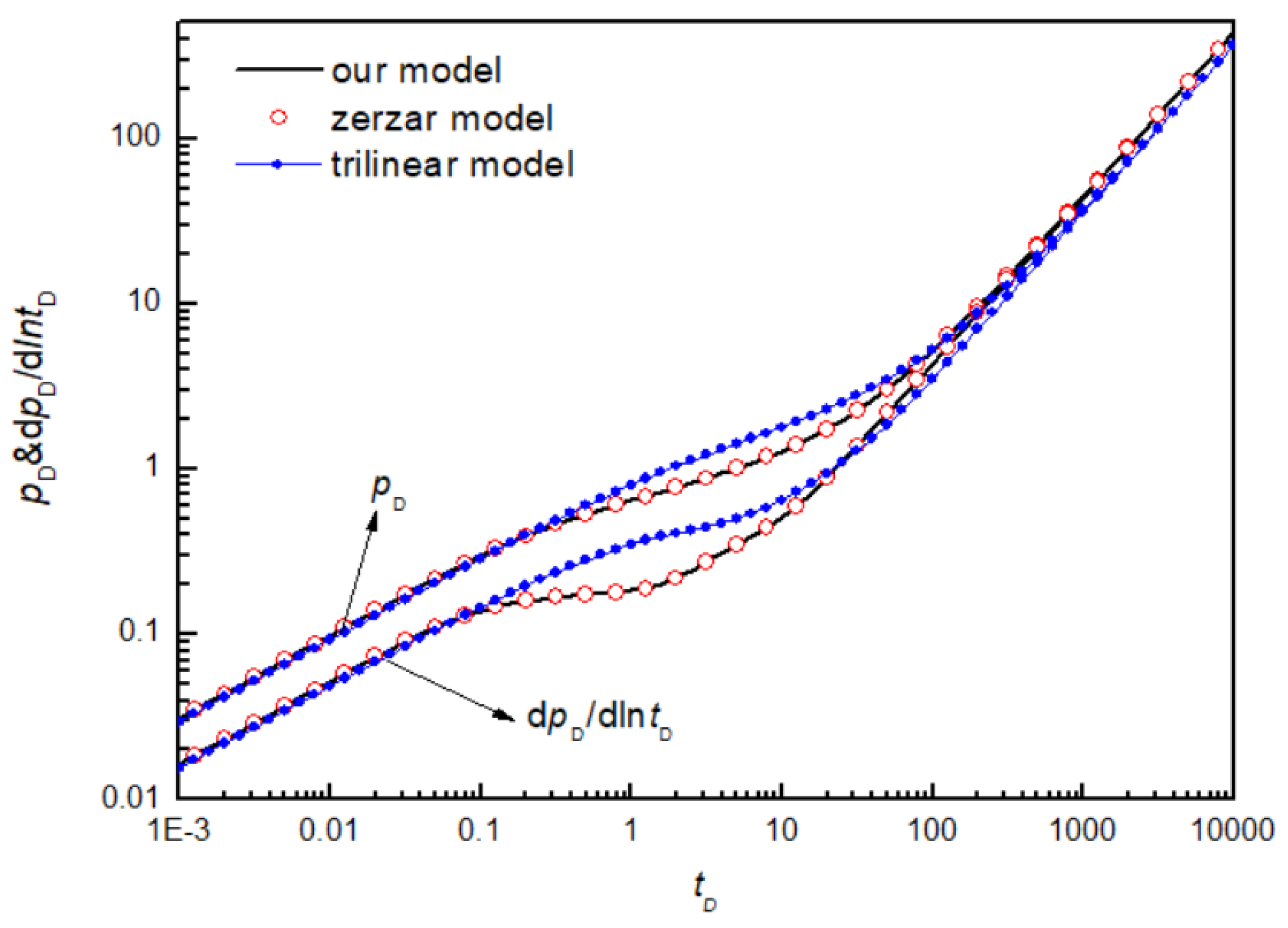
4. Comparison and Verification

In order to verify the accuracy of our model, a relatively simple model of MFHW is discussed, which located in the center of a closed, homogenous- and single-porosity media, rectangular reservoir with three blocks. The transient pressure performance of MFHW in homogeneous reservoirs is calculated by [24] using the source function and the principle of superposition method. The properties of the hydraulic fractures and reservoir are given in

Table 1. Values of well and reservoir parameters.

Parameters	Value	Unit
Reference length, ℓ	100	m
Hydraulic fracture number	3	-
Reservoir size in x, y-direction xe, ye	1200	m
Each block size in x, y direction, xei, yei	400	m
Half-length of each hydraulic fracture, Lfi	60	m
Formation thickness, h	100	m
hydraulic fracture height, hfi	100	m
Natural fracture permeability, kfi	100	mD
Matrix Permeability, km	1	mD
Initial pressure	35	MPa
elastic storage ratio ωfi	0.1	-
crossflow coefficient λfi	2	-

, and the results with different discretized number m_e (Figure 3) are shown in

Table 2. Comparison of the model results with different segments of block interfaces.

tD	Zerar 2004		me = 1		me = 2		me = 3		me = 4
	pD	dpD/dlntD	pD	dpD/dlntD	pD	dpD/dlntD	pD	dpD/dlntD	pD	dpD/dlntD
0.001	0.031139	0.016465	0.031139	0.016465	0.031139	0.016465	0.031139	0.016465	0.031139	0.016465
0.01	0.098465	0.052051	0.098465	0.052051	0.098465	0.052051	0.098465	0.052051	0.098465	0.052051
0.1	0.298781	0.138895	0.298781	0.138895	0.298781	0.138895	0.298781	0.138895	0.298781	0.138895
1	0.644286	0.184087	0.644049	0.183229	0.644049	0.183229	0.644049	0.183229	0.644049	0.183229
10	1.289051	0.50975	1.285585	0.509678	1.285585	0.509678	1.285585	0.509678	1.285585	0.509678
100	5.237377	4.36373	5.237641	4.366273	5.237641	4.366273	5.237641	4.366273	5.237641	4.366273
1000	44.5198	43.70941	44.53383	43.78088	44.53383	43.78088	44.53383	43.78088	44.53383	43.78088
10,000	437.4155	437.3679	437.1711	435.6028	437.1711	435.6028	437.1711	435.6028	437.1711	435.6028
Errors	-	-	0.0664%	0.2043%	0.0654%	0.2003%	0.065%	0.2001%	0.065%	0.2001%

and plotted in Figure 4.

Table 2 presents the comparisons of our models with Zerzar’s model about pressure and pressure derivatives. Four cases of different interface discretization between the blocks are shown in Figure 3. Table 2 demonstrates that there are almost no differences among the four cases. All of them can match the Zerzar’s model very well. The maximum error (m_e = 1) between the Zerzar’s model and our model is 0.0664% of dimensionless pressure drop, 0.2043% of dimensionless pressure derivative, which is too small to be distinguished on the log-log plot of Figure 4, which shows high correctness of our model. To simplify the calculation process, we assumed m_e = 1 for the following discussion.

In Figure 4, the flow stages of MFHW can be identified including first linear flow, first radial flow and late pseudo-steady boundary flow, which are different from traditional MFHWs flow regimes. As hydraulic fractures are close to the impermeable boundaries in our model, the second linear and radial flows do not appear. In addition, we compare our model with trilinear flow model [6], which is widely used for unconventional reservoir because of its concise formula and convenient calculation. In Figure 4, it shows that the pressure and pressure derivative of our model can be matched perfectly with trilinear model at first linear flow and late pseudo-steady boundary flow period. However, radical flow around each hydraulic fracture is missing in trilinear flow model, which is not in line with real situation. Therefore, our model is more accurate than trilinear flow model.

5. Results and Discussion

The semi-analytical pressure solution for MFHWs within some rectangular reservoir blocks of different parameters is obtained. This section presents pressure behavior and flux distribution of each hydraulic fracture with some heterogeneous parameters. We assume that there are three compartments of the reservoir, the horizontal well penetrates these three compartments and there are three hydraulic fractures in the middle of each block. Besides the basic properties given in Table 1, the parameters in dual porosity media includes elastic storage ratio ${\omega }_f=0.1$ and crossflow coefficient ${\lambda }_f=2$. The heterogeneous parameter ratio values of three blocks are shown in

Table 3. The heterogeneous parameter ratio of three blocks.

Parameters	Case 1	Case 2	Case 3	Case 4	Case 5
$k_{f1}:k_{f2}:k_{f3}$	1:1:1	1:2:1	1:1/2:1	1:2:3	1:1/2:1/4
$x_{e1}:x_{e2}:x_{e3}$	1:1:1	1:2:1	1:1/2:1	-	-
${\omega }_{f1}:{\omega }_{f2}:{\omega }_{f3}$	1:1:1	1:2:1	1:2:3	-	-
${\lambda }_{f1}:{\lambda }_{f2}:{\lambda }_{f3}$	1:1:1	1:2:1	1:2:3	-	-
$L_{f1}:L_{f2}:L_{f3}$	1:1:1	1:2:1	2:1:2	-	-

.

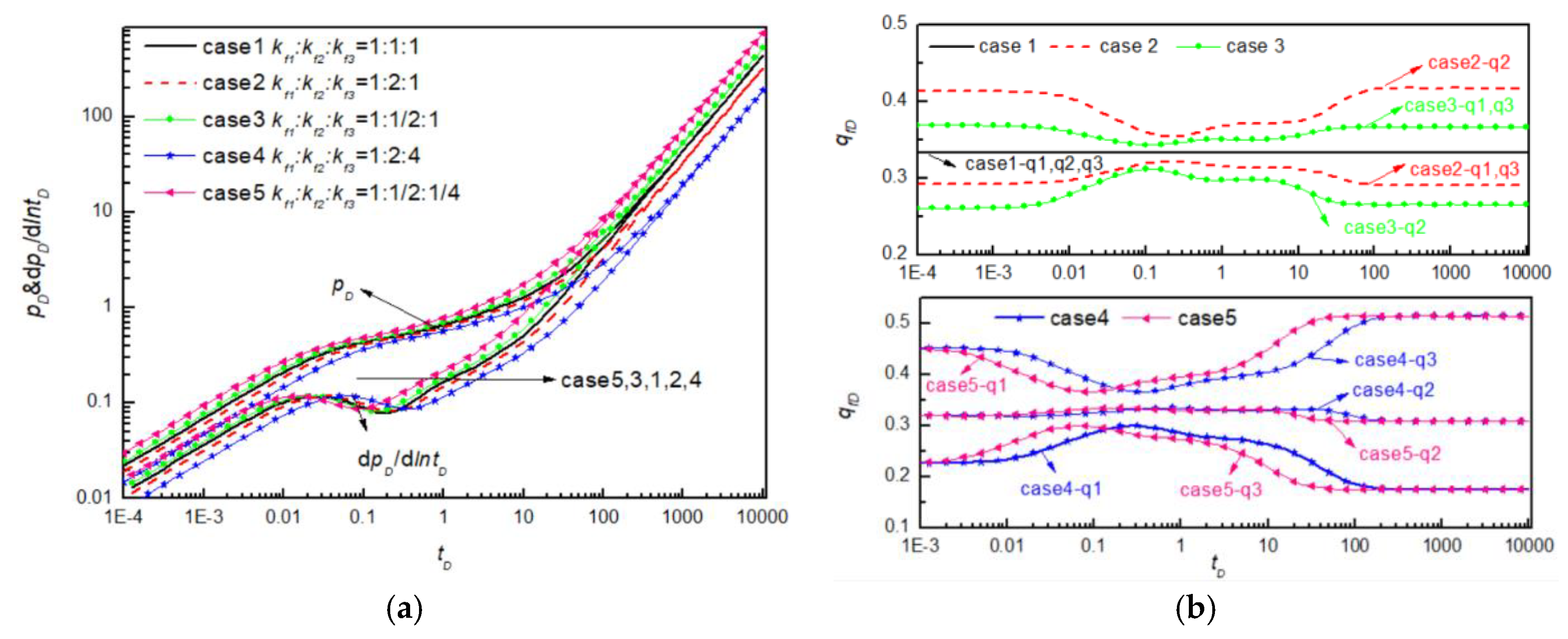
5.1. Heterogeneous Permeability

We consider five cases of heterogeneous permeability distribution, and the natural fracture permeability ratio of these three blocks is shown in Table 3. In cases 2 and 4, the permeability increases in second and third compartment, while in cases 3 and 5, the permeability decreases in second and third compartment. Figure 5 shows the pressure and pressure derivative responses as well as the flux distribution of three different hydraulic fractures.

In Figure 5a, for the pressure-transient responses, we can see that the heterogeneous permeability distribution of different drainage blocks affects both arriving time and the pressure drop of the whole MFHW flow regimes including first linear flow, crossflow regime, first radial flow and late pseudo-steady boundary flow. The higher the permeability of cases 2 and 4, the earlier different regimes arrive, and the less the pressure drop compared with reference case 1 (homogeneous permeability), which is beneficial to production. On the contrary, with the lower permeability of cases 3 and 5, the higher-pressure transient curve means more pressure drop demands for constant flow rate condition of horizontal wellbore. Figure 5b shows the effect of heterogeneous permeability on the flux of each fracture. As shown in Figure 5b, there are great differences between different fracture fluxes with unequal permeability distribution. In homogeneous permeability case 1, the flux of each fracture is equal to q_total/3. For the other heterogeneous permeability cases, the flux of fractures in higher permeability blocks is larger during the early linear flow period. Then, the difference will decrease because of crossflow between each block. Finally, the differences will become stable in the last pseudo-steady boundary period. Simultaneously, for lower-permeability case 5, the crossflow period appears earlier compared to the higher-permeability case 4, which is the same as the pressure response in Figure 5a.

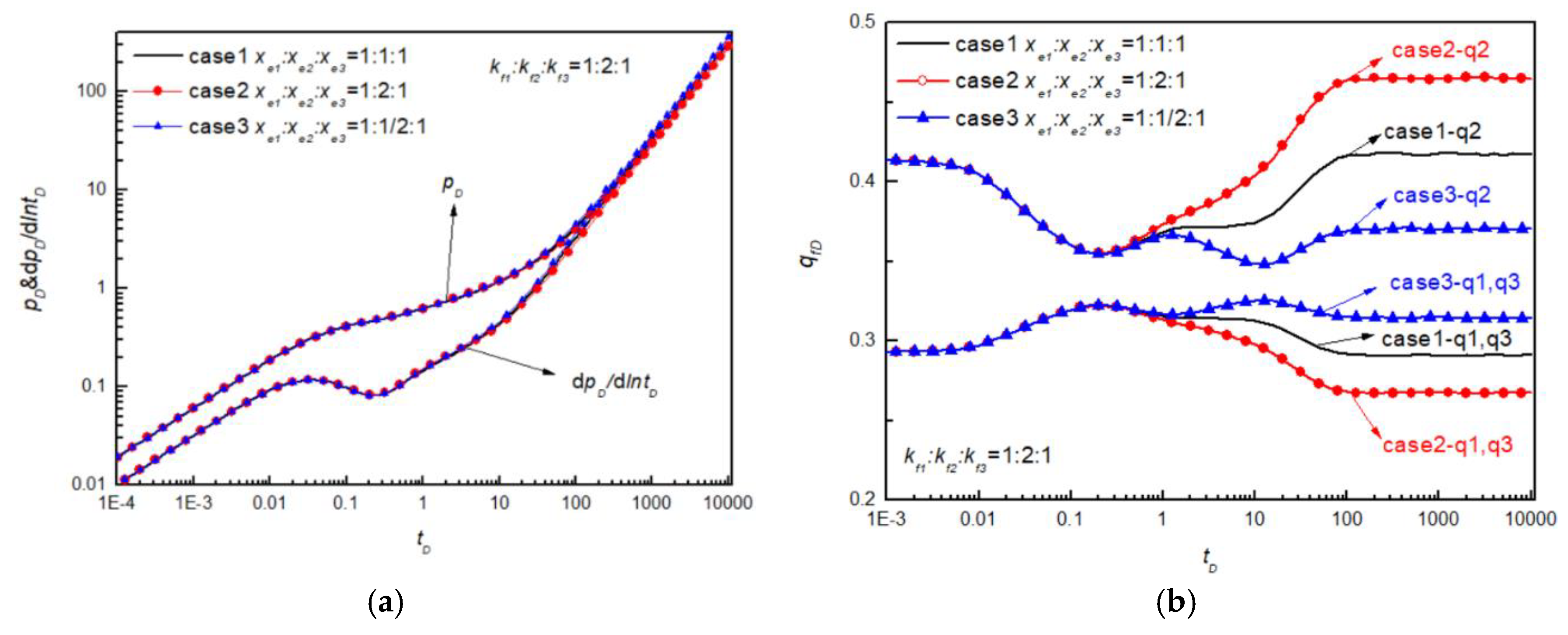
5.2. Non-Uniform Length of Blocks

To consider the non-uniform length distribution effect, we use a heterogeneous permeability model with k_f1:k_f2:k_f3 = 1:2:1. Three different cases with unequal length distributions of each compartment are considered in Table 3 under the constant whole drainage length condition. Then, the pressure response and flux distribution are shown in Figure 6.

From Figure 6a, we can see that if the whole drainage length is constant, the dimensionless pressure drop and pressure derivative curves have no change when the drainage length of each fracture is different. However, in Figure 6b, the flux distribution of each fracture is different after considering the block length heterogeneity. Non-uniform block length only affects the final flux proportion of each fracture. It has no effect on the arriving time to the crossflow and last pseudo-steady flow period. In other words, there is no obvious effect on the wellbore pressure drop when the partial section area is damaged or stimulated in the same drainage area, which only affect the flux proportion of each fracture.

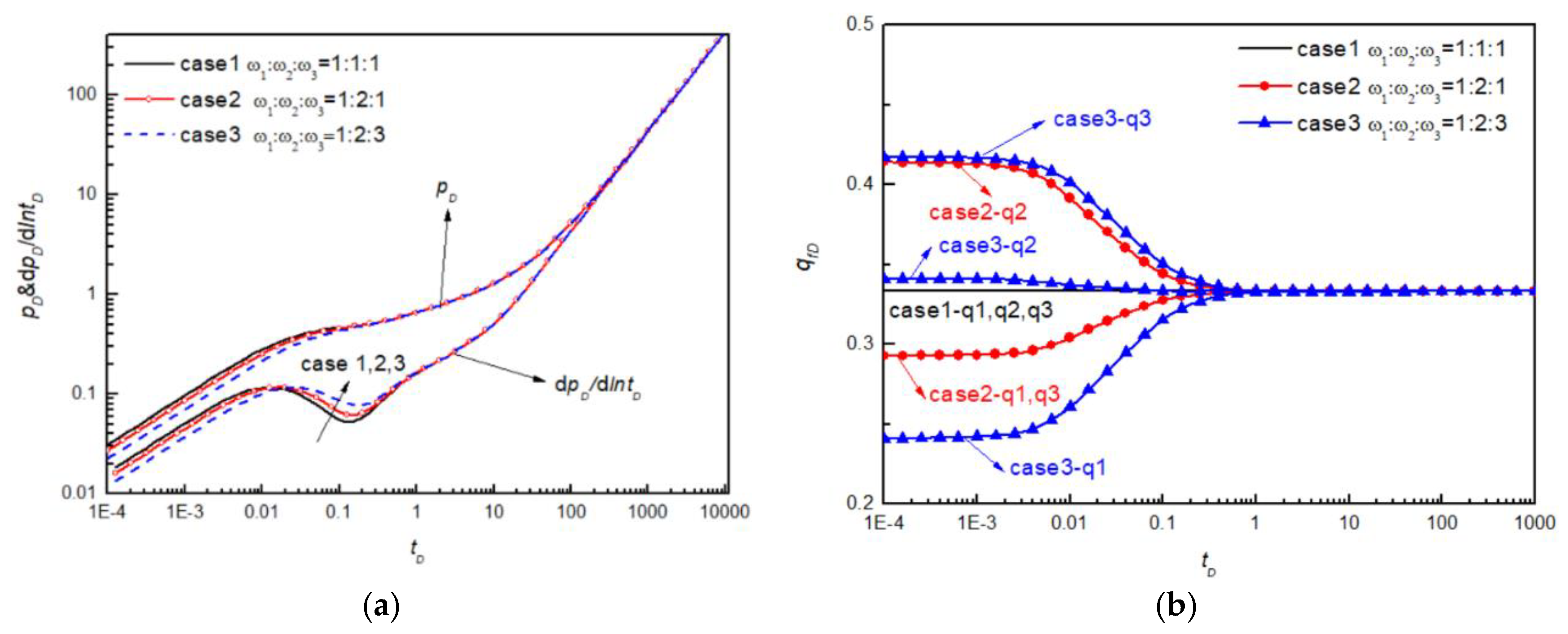
5.3. Different Elastic Storage Ratio

To consider the different elastic storage ratio effect of each block in drainage area, three cases are considered in Table 3, and corresponding pressure and flux curves are shown in Figure 7.

Figure 7a illustrates that the elastic storage ratio between different drainage blocks mainly affects the first linear flow, first radial flow and crossflow regimes. When the elastic storage ratio increases from case 1 to case 2 and case 3, which means the storage capacity of natural fracture system is greater and more fluid is stored in the natural fractures, the dimensionless pressure derivative curves show smaller groove because of less fluid transfer between natural fractures and matrix. From Figure 7b, it shows the same performance as pressure response. The flux distribution is only affected in the early stages, while the flux of each fracture converges to the same q_total/3 at the later pseudo-steady flow period. Similarly, the less natural fracture storage capacity ω, the less corresponding flux of hydraulic fracture.

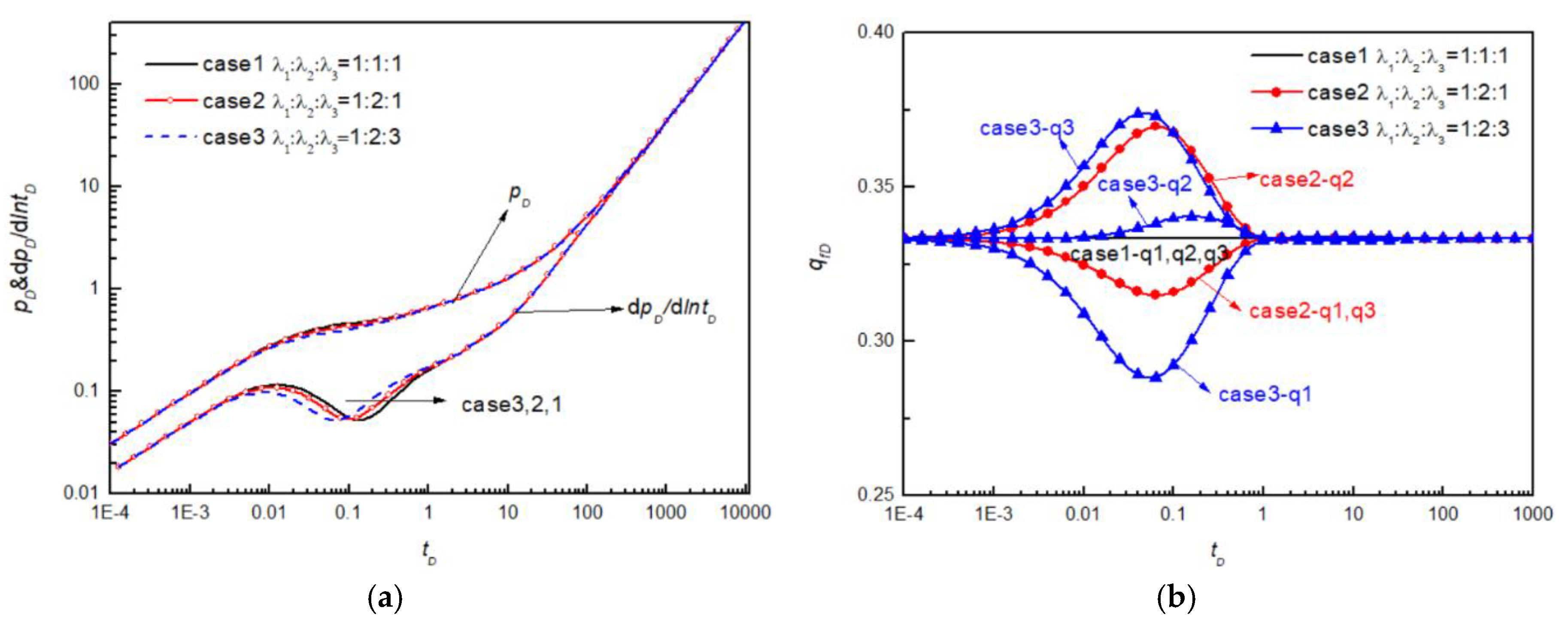
5.4. Different Crossflow Ratio

Another important parameter of dual porosity for naturally fracture system is crossflow ratio. Three cases are investigated in Table 3, and the pressure responses and flux distribution are shown in Figure 8.

The crossflow ratio represents the fluid flowing ability from the matrix to the natural fracture system. As shown in Figure 8, the different crossflow ratio only affects crossflow stage in the pressure responses and flux distribution. The larger λ value of the block is, the earlier the crossflow appears between different cases and the higher the flux is during the crossflow period.

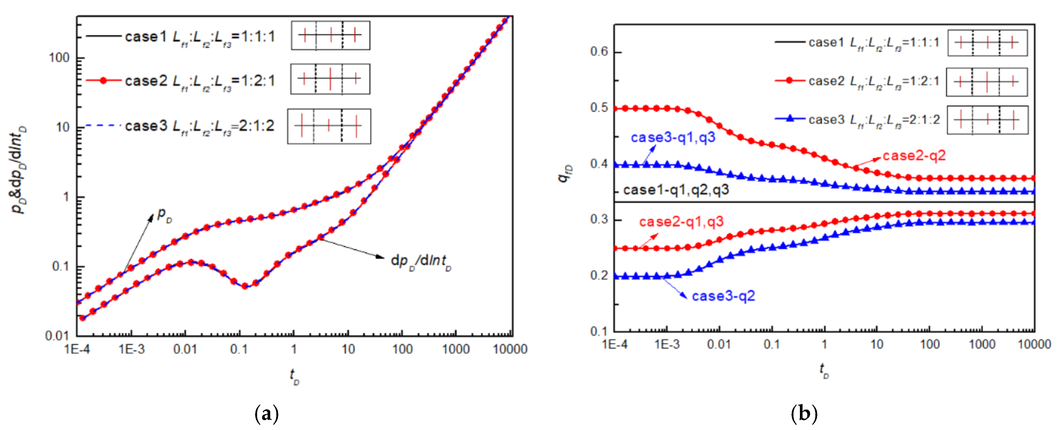
5.5. Non-Uniform Half-Length Distribution of Fractures

With the constant total fracture length, we consider three cases of non-uniform fracture half-length distribution. The ratio of three hydraulic fracture half-lengths is shown in Table 3. Figure 9 gives the pressure response and flux distribution.

From Figure 9a, we can see that if the total fracture half-length is constant, pressure response curves have nothing to do with different half-length distribution. However, In Figure 9b, the flux distribution of each fracture is changed by half-length heterogeneity. The flux difference between each fracture becomes smaller as the flow time increases, and becomes stable gradually after crossflow stages.

6. Conclusions

This work investigates the pressure transient solutions of MFHWs in heterogeneous systems where the sections of the naturally fractured reservoir display different characteristics. A semi-analytical method is presented which combines source function and boundary element method. Major conclusions are summarized below:

(1)

This model only discretizes hydraulic fractures and interface boundaries. With a small number of segments interface discretization, it can match verified model very well on the log–log plots. As a result, this model can greatly reduce fine gridding required by numerical approach.

(2)

Compared to the trilinear flow model, this model can consider the radial flow around the hydraulic fracture, and the interference effect between hydraulic fractures with different formation properties.

(3)

As the permeability increases along the horizontal well direction, the pressure drop decreases and flow regimes become earlier. The fractures flux fluctuates with flow regimes, where the difference between high- and low-permeability blocks decreases firstly, then increases gradually, and tends to be stable finally. When the entire drainage length keeps constant, the pressure responses have nothing to do with non-uniform heterogeneous block length while flux distribution has been changed obviously.

(4)

The elastic storage ratio mainly affects the early flow regimes including first linear flow, first radial flow and crossflow periods. The bigger the elastic storage ratio, the smaller the groove and the greater the flux. However, the crossflow ratio only affects the crossflow period. The bigger the crossflow ratio, the earlier the crossflow arrives.

References

1. Soliman, M.; Daal, J.; East, L. Fracturing unconventional formations to enhance productivity. J. Nat. Gas Sci. Eng. 2012, 8, 52–67. [Google Scholar] [CrossRef]
2. Nguyen-Le, V.; Shin, H. Development of reservoir economic indicator for Barnett Shale gas potential evaluation based on the reservoir and hydraulic fracturing parameters. J. Nat. Gas Sci. Eng. 2019, 66, 159–167. [Google Scholar] [CrossRef]
3. Dian, F.; Amin, E. Semi-analytical modeling of shale gas flow through fractal induced fracture networks with micro-seismic data. Fuel 2017, 193, 444–459. [Google Scholar]
4. Fan, D.Y.; Yao, J.; Sun, H.; Zeng, H.; Wang, W. A composite model of hydraulic fractured horizontal well with stimulated reservoir volume in tight oil & gas reservoir. J. Nat. Gas Sci. Eng. 2015, 24, 115–123. [Google Scholar]
5. Zhao, Y.; Zhang, L.-H.; Luo, J.-X.; Zhang, B.-N. Performance of fractured horizontal well with stimulated reservoir volume in unconventional gas reservoir. J. Hydrol. 2014, 512, 447–456. [Google Scholar] [CrossRef]
6. Brown, M.; Ozkan, E.; Ragahavan, R.; Kazemi, H. Practical solutions for pressure transient responses of fractured horizontal wells in unconventional reservoirs. SPE Res. Eval. Eng. 2011, 14, 663–676. [Google Scholar] [CrossRef]
7. Stalgorova, E.; Mattar, L. Practical analytical model to simulate production of horizontal wells with branch fractures. In Proceedings of the SPE Paper 162515 Presented at SPE Canadian Unconventional Resources Conference, Calgary, AB, Canada, 30 October–1 November 2012. [Google Scholar]
8. Stalgorova, K.; Mattar, L. Analytical model for unconventional multi-fractured composite systems. SPE Reserv. Eval. Eng. 2013, 16, 246–256. [Google Scholar] [CrossRef]
9. Guo, J.; Zeng, J.; Wang, X. Analytical model for multi-fractured horizontal wells in heterogeneous shale reservoirs. In Proceedings of the SPE Asia Pacific Oil & Gas Conference and Exhibition, Society of Petroleum Engineers (SPE), Perth, Australia, 25–27 October 2016. [Google Scholar]
10. Ozcan, O.; Sarak, H.; Ozkan, E.; Raghavan, R. A trilinear flow model for a fractured horizontal well in a fractal unconventional reservoir. In Proceedings of the SPE Paper 170971 Presented at SPE Annual Technical Conference and Exhibition, Amsterdam, The Netherlands, 27–29 October 2014. [Google Scholar]
11. Wang, W.; Su, Y.; Sheng, G.; Cossio, M.; Shang, Y. A mathematical model considering complex fractures and fractal flow for pressure transient analysis of fractured horizontal wells in unconventional reservoirs. J. Nat. Gas Sci. Eng. 2015, 23, 139–147. [Google Scholar] [CrossRef]
12. Salam, A.R.; Tiab, D. Partially penetrating hydraulic fractures: Pressure responses and flow dynamics. In Proceedings of the SPE Paper 164500 Presented at SPE Production and Operation Symposium, Oklahoma City, OK, USA, 23–26 March 2013. [Google Scholar]
13. Zawila, J.; Fluckiger, S.; Hughes, G.; Kerr, P.; Hennes, A.; Hofmann, M. An integrated, multi-disciplinary approach utilizing stratigraphy, petro-physics, and geophysics to predict reservoir properties of tight unconventional sandstones in the Powder River basin, Wyoming, USA. In Proceedings of the SEG Paper 5852423 Presented at SEG Annual Meeting, New Orleans, LA, USA, 19–20 August 2015. [Google Scholar]
14. Liu, P.; Ju, Y.; Ranjith, P.G.; Zheng, Z.; Chen, J. Experimental investigation of the effects of heterogeneity and geostress difference on the 3D growth and distribution of hydro-fracturing cracks in unconventional reservoir rocks. J. Nat. Gas Sci. Eng. 2016, 35, 541–554. [Google Scholar] [CrossRef]
15. Karimi-Fard, M.; Durlofsky, L.J.; Aziz, K. An efficient Discrete-Fracture model applicable for general-purpose reservoir simulators. In Proceedings of the SPE Paper 79699 Presented at SPE Reservoir Simulation Symposium, Houston, TX, USA, 3–5 February 2004. [Google Scholar]
16. Warpinski, N.; Mayerhofer, M.; Vincent, M.; Cipolla, C.; Lolon, E. Stimulating Unconventional Reservoirs: Maximizing Network Growth While Optimizing Fracture Conductivity. J. Can. Pet. Technol. 2009, 48, 39–51. [Google Scholar] [CrossRef]
17. Yan, X.; Huang, Z.; Yao, J.; Li, Y.; Fan, D. An efficient embedded discrete fracture model based on mimetic finite difference method. J. Pet. Sci. Eng. 2016, 145, 11–21. [Google Scholar] [CrossRef]
18. Gringarten, A.C.; Ramey, H.J. The Use of Source and Green’s Functions in Solving Unsteady-Flow Problems in Reservoirs. Soc. Pet. Eng. J. 1973, 13, 285–296. [Google Scholar] [CrossRef]
19. Chen, C.-C.; Rajagopal, R. A Multiply-Fractured Horizontal Well in a Rectangular Drainage Region. SPE J. 1997, 2, 455–465. [Google Scholar] [CrossRef]
20. Guo, G.; Evans, R.D. Pressure-transient behavior and inflow performance of horizontal wells intersecting discrete fractures. In Proceedings of the SPE paper 26446 Presented at SPE Annual Technical Conference and Exhibition, Houston, TX, USA, 3–6 October 1993. [Google Scholar]
21. Ozkan, E.; Raghavan, R. New Solutions for Well-Test-Analysis Problems: Part 1-Analytical Considerations (includes associated papers 28666 and 29213 ). SPE Form. Eval. 1991, 6, 359–368. [Google Scholar] [CrossRef] [Green Version]
22. Özkan, E.; Raghavan, R. New Solutions for Well-Test-Analysis Problems: Part 2 Computational Considerations and Applications. SPE Form. Eval. 1991, 6, 369–378. [Google Scholar] [CrossRef]
23. Jia, P.; Cheng, L.; Huang, S.; Wu, Y. A semi-analytical model for the flow behavior of naturally fractured formations with multi-scale fracture networks. J. Hydrol. 2016, 537, 208–220. [Google Scholar] [CrossRef]
24. Zerzar, A.; Bettam, Y. Interpretation of multiple hydraulically fractured horizontal wells in closed systems. In Proceedings of the SPE Paper 84888 Presented at SPE International Improved Oil Recovery Conference in Asia Pacific, Kuala Lumpur, Malaysia, 8–10 June 2003. [Google Scholar]
25. Zhao, Y.; Zhang, L.-H.; Zhao, J.-Z.; Luo, J.-X.; Zhang, B.-N. “Triple porosity” modeling of transient well test and rate decline analysis for multi-fractured horizontal well in shale gas reservoirs. J. Pet. Sci. Eng. 2013, 110, 253–262. [Google Scholar] [CrossRef]
26. Xu, J.; Guo, C.; Wei, M.; Jiang, R. Production performance analysis for composite shale gas reservoir considering multiple transport mechanisms. J. Nat. Gas Sci. Eng. 2015, 26, 382–395. [Google Scholar] [CrossRef]
27. Zeng, H.; Fan, D.; Yao, J.; Sun, H. Pressure and rate transient analysis of composite shale gas reservoirs considering multiple mechanisms. J. Nat. Gas Sci. Eng. 2015, 27, 914–925. [Google Scholar] [CrossRef]
28. Kikani, J.; Horne, R.N. Modeling Pressure-Transient Behavior of Sectionally Homogeneous Reservoirs by the Boundary-Element Method. SPE Form. Eval. 1993, 8, 145–152. [Google Scholar] [CrossRef]
29. Idorenyin, E.H.; Shirif, E. Transient response in arbitrary-shaped composite reservoirs. SPE Res. Eval. Eng. 2016, 9, 1–13. [Google Scholar] [CrossRef]
30. Medeiros, F.; Özkan, E.; Kazemi, H. A Semianalytical Approach to Model Pressure Transients in Heterogeneous Reservoirs. SPE Reserv. Eval. Eng. 2010, 13, 341–358. [Google Scholar] [CrossRef]
31. Mayerhofer, M.J.; Lolon, E.; Warpinski, N.R.; Cipolla, C.L.; Walser, D.W.; Rightmire, C.M. What Is Stimulated Reservoir Volume? SPE Prod. Oper. 2010, 25, 89–98. [Google Scholar] [CrossRef]
32. Carslaw, H.S.; Yaeger, J.C. Conduction of Heat in Solids; Oxford University Press: Oxford, UK, 1959. [Google Scholar]
33. Stehfest, H. Numerical Inversion of Laplace Transforms. Commun. ACM 1970, 13, 47–49. [Google Scholar] [CrossRef]
Figure 1. Multiple fractured horizontal wells (MFHWs) through a compartmentalized heterogeneous reservoir.
Energies 13 05204 g001
Figure 2. A plane perpendicular to the x-axis in the rectangular parallelepiped. (a) One block with hydraulic fracture; (b) the fracture plane.
Energies 13 05204 g002
Figure 3. Different discretization schemes at the block interfaces.
Energies 13 05204 g003
Figure 4. Model verification of Zerzar model and our model (nf = 3, me = 1).
Energies 13 05204 g004
Figure 5. Pressure response and flux distribution of heterogenous permeability. (a) Pressure and pressure derivative; (b) flux distribution of each hydraulic fracture.
Energies 13 05204 g005
Figure 6. Pressure response and flux distribution of non-uniform length distribution. (a) Pressure and pressure derivative; (b) Flux distribution of each hydraulic fracture.
Energies 13 05204 g006
Figure 7. Pressure response and flux distribution of different elastic storage ratio. (a) Pressure and pressure derivative; (b) Flux distribution of each hydraulic fracture.
Energies 13 05204 g007
Figure 8. Pressure response and flux distribution of different crossflow ratio. (a) Pressure and pressure derivative; (b) Flux distribution of each hydraulic fracture.
Energies 13 05204 g008
Figure 9. Pressure response and flux distribution of different half-length distribution. (a) Pressure and pressure derivative; (b) Flux distribution of each hydraulic fracture.
Energies 13 05204 g009