Abstract
In comparison to high-voltage alternating current (HVAC) cable systems, high-voltage direct current (HVDC) systems have several advantages, e.g., the transmitted power or long-distance transmission. The insulating materials feature a non-linear dependency on the electric field and the temperature. Applying a constant voltage, space charges accumulate in the insulation and yield a slowly time-varying electric field. As a complement to measurements, numerical simulations are used to obtain the electric field distribution inside the insulation. The simulation results can be used to design HVDC cable components such that possible failure can be avoided. This work is a review about the simulation of the time-varying electric field in HVDC cable components, using conductivity-based cable models. The effective mechanisms and descriptions of charge movement result in different conductivity models. The corresponding simulation results of the models are compared against measurements and analytic approximations. Different numerical techniques show variations of the accuracy and the computation time that are compared. Coupled electro-thermal field simulations are applied to consider the environment and its effect on the resulting electric field distribution. A special case of an electro-quasistatic field describes the drying process of soil, resulting from the temperature and electric field. The effect of electro-osmosis at HVDC ground electrodes is considered within this model.
1. Introduction
For the transmission of high electric power over long distances, high-voltage direct current (HVDC) is used due to less losses in comparison to high-voltage alternating current (HVAC) [1]. Vanishing capacitive and inductive losses in HVDC power cables result in no theoretical limit for the cable length. A HVDC cable system consists of the cable itself, the cable joint and the cable termination. The cable joint is used to connect two cable segments. Cable terminations are installed at the end of a cable or connected e.g., to a “gas-insulated substation” (GIS) [1,2,3,4].
Worldwide HVDC projects show that the two main insulation materials are mass-impregnated paper (MI) and extruded materials. Extruded insulations are polymeric materials such as different types of polyethylene (PE), e.g., “cross-linked polyethylene” (XLPE) or “low-density polyethylene” (LDPE). The applications of extruded cables have increased in recent years due to significant advantages in manufacturing, installation, transportation and maintenance [5]. The world’s first HVDC cable was put into service in 1954, with a voltage of 80 kV and an insulation of MI. Polymeric insulation materials appeared in the late 1960s and have been used for HVAC cables. In 1999, the first commercial polymeric HVDC cable was put into service, with a voltage of 80 kV [6,7]. Today, the voltage has increased up to 640 kV and modern HVDC cables commonly consist of XLPE, but due to their high reliability, MI cables are still in service [1,3,8,9].
Both insulations, MI and XLPE have a non-linear electric conductivity that depends on many factors, where the most important ones are the temperature and the electric field [3,8,10]. The applied voltage results in generated heat, due to the current in the conductor and a leakage current within the insulation. Both heat losses yield a temperature gradient within the insulation [11]. Due to the applied voltage and the temperature, a space charge density accumulate within the insulating material [12]. The electric field of the accumulated space charges superimpose the applied electric field and the total electric field varies in time. Using the time constant,
where ε0 = 8.854 × 10⁻¹² As/(Vm) is the dielectric constant, εr is the relative permittivity and is the electric field and temperature T dependent electric conductivity, a stationary electric field is obtained at approximately 10∙τ. Due to the non-linear electric conductivity, a stationary field may be obtained after hours or weeks [1,3,13,14]. For example, Figure 1a shows the electric field within a MI insulation with conductor temperature T(ri) = Ti = 55 °C, sheath temperature T(ra) = Ta = 35 °C and applied voltage U = 450 kV. A stationary electric field is seen above the black dashed line. The cylindrical geometry is depicted in Figure 1b, where the electric field is computed along the red evaluation line due to its radial dependency only [11,13].
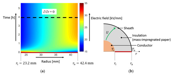
Figure 1.
(a) Time-dependent electric field within a mass-impregnated paper (MI) insulation. The stationary electric field is obtained above the black dashed line; (b) geometry of the cylindrical insulation. The electric field is computed along the red evaluation line [11,13].
During the operation time, the electric field varies from a purely capacitive field (t = 0), determined by the permittivity, to a purely resistive field (t ≈ 4 h), determined by the electric conductivity [11]. With accumulated space charges, the electric field decreases in the vicinity of the conductor and increases near the sheath, called the “inversion of field” [8]. Due to the field-changing behavior of accumulated space charges, the electric field may exceed the breakdown strength of the dielectric that can cause reliability problems or failure of HVDC cable components. Furthermore, high electric field values and increased losses within the insulation may result in a thermal breakdown [1,15,16].
In addition to measurements, numerical simulations are used to determine the space charge and electric field distribution inside the insulation. The simulated electric field and charge distribution can be used to prevent HVDC cable components from possible failure.
In the last years, several research and review papers (e.g., [1,4,11,15]) have been published within the field of HVDC cables systems, where the modeling and the numerical simulation of the electric field are mainly of minor interest. Different conductivity models and simulation methods are found throughout the literature. This work is a review about the simulation of the time-varying electric field in HVDC cable components, using conductivity-based cable models. Based on the effective mechanisms and descriptions of charge movement, different conductivity models are presented. With a comparison of the simulation results against measurements and analytic solutions, the main results of the electric field in HVDC cable systems are summarized.
The simulation of the electric field under constant stress covers various topics, which makes it necessary to divide this paper into several parts. After the introduction, the next section consists of the charge movement within the insulations and the resulting non-linear electric conductivity. Section 3 gives a short review about the accumulation of charges and their influence on the electric field. The necessary equations and possible pseudo codes to obtain the electric and thermal fields are described in Section 4. Simulation results of the time-varying and the stationary electric fields are presented in Section 5. The results in Section 5 neglect the effect of interfaces or moving charges, which are seen in Section 6. A comparison between different simulation techniques, focusing the simulation time and the accuracy, is presented in Section 7. A special case of a time-varying electric field in the vicinity of ground electrodes is described in Section 8, followed by the conclusions and an outlook into further research areas in Section 9.
2. High-Voltage Direct Current (HVDC) Cable Insulation Materials and the Non-Linear Electric Conductivity
MI as insulation material consists of high-density paper that is lapped and then impregnated with a high-viscosity mineral oil [5]. XLPE and LDPE are based on PE, where e.g., XLPE is manufactured within an additional cross-linking process. PE is a semicrystalline polymer that consists of amorphous and crystalline regions. Within the crystalline regions, polymer chains contain an orderly configuration and align themselves in crystalline lamellae. During the crystallization, many lamellae may grow from a single nucleus and form a spherulite within which the lamellae are radially aligned. The amorphous regions between the lamellae and spherulites, consists e.g., of chain ends or branches [3,17,18,19]. The final insulation material consists of the dielectric (PE) and two semiconducting layers (semicon), where all three layers are usually extruded within the same production step [1].
Using the band diagram to describe both materials, single states (traps) form the conduction band and the valence band, resulting in a mean band gap energy W. These traps are the result of oil and cellulose molecules in MI, the semicrystalline structure of PE and different impurities that are seen in both insulations, coming from the manufacturing process. Charges are caught within the traps and facing a potential barrier, when trying to escape. For example, the band diagram of XLPE is seen in Figure 2a, where charges are trapped and released.
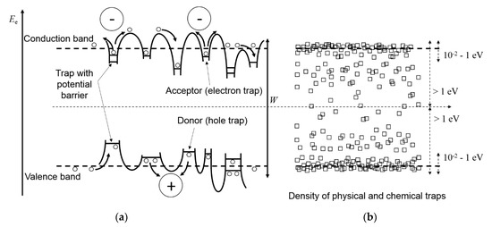
Figure 2.
(a) Band structure for an insulation material like cross-linked polyethylene (XLPE), where states with different energy levels are formed due to the semicrystalline structure of polyethylene (PE) and impurities within the material. Because of these states, only a mean band gap energy W is defined; (b) density of traps as a function of the trap depth. A high density of shallow traps (trap depth 10−2–1 eV) is seen near the conduction band and the valence band. With increasing trap depth and thus distance to the conduction band and the valence band, the trap density is decreasing [17,20,21].
The traps are called “physical traps” or “shallow traps” and “chemical traps” or “deep traps”, depending on the trap depth. For XLPE, shallow traps have a depth of 10−2–1 eV, while the depth of deep traps is >1 eV [17,20,21]. The density of the traps is high near the conduction and valence band and decreases with increasing distance, as illustrated in Figure 2b.
Depending on the trap depth ETrap, charges remain in traps that may range from a few seconds to years. The time tTrap is given by:
where kB = 1.38 × 10⁻²³ J/K is the Boltzmann constant and 1/tTrap,0 ≈ (kB∙T)/hP is the “escape frequency”, with hP = 6.626 × 10⁻³⁴ Js as the Plank constant [17,20,22,23,24].
Charges correspond to the conduction mechanism if they are released from traps. Consider one charge within a trap, facing a potential barrier. With a sufficiently high temperature, the charge has enough energy to escape. This process is supported by an external electric field that lowers the potential barrier in the direction of the field, resulting in the characteristic sinh-dependency of the electric field [10,23]. In general, the electric conductivity depends on many factors, e.g., the morphology, the local electric field and temperature or the humidity. In literature, the conductivity is commonly given with a dependency on the local electric field and temperature only (see e.g., [14,17,20,23,25]), which are the most important factors [26].
With (2), the electric conductivity is described by:
where EA,1 is the activation energy and K1 and γ1 are constants. All three constants EA,1, K1 and γ1 are determined by measurements [17,22,23,27]. In [3,14,28,29], the temperature dependency within the hyperbolic sine is neglected and the conductivity is described by:
where EA,2, K2 and γ2 are different constants. The electric conductivity in (3) and (4) is based on the hopping theory. Using the Poole–Frenkel effect, the conductivity is described by:
and similar to (3) and (4), whereas the dependence on the electric field differs [17,20]. In (5), the constants are EA,3, K3 and γ3 that have to be determined by measurements as well. The conductivity models in (3)–(5) are described by analogies to the semiconductor technology. Based on worldwide experience and a narrow range of the operation temperature, the electric conductivity is commonly given in a double exponential form with:
where the constants are κ0, α and β [22,30,31,32]. For MI, α ≈ 0.1 °C−1 and β ≈ 0.03 mm/kV [30]. In the case of XLPE, α ≈ 0.1 °C−1 and β ≈ 0.1 mm/kV [31]. Thus, the temperature dependency of both materials is approximately equal, but the electric field dependency is 3.5 times higher in XLPE [22,30,31]. A different formulation of (6) is:
where the constants κ0 and α are equal to (6), but the electric field dependency is determined by the constants ERef and v. Considering a cable geometry, as depicted in Figure 1b, the approximations ERef = U∙exp(−1)/(ra − ri) and v = U∙β/(ra − ri), with ri as the radius of the conductor and ra as the radius of the sheath, hold true [25,26,30].
There is still a gap of knowledge to describe the charge transport and the electric conductivity of the insulating material in detail, due to the complex morphology. This results in many different possibilities to describe non-linear variations over temperature and electric field. In [33], further conductivity models are shown. The conductivity models (3)–(7) are valid for high field conduction ( > 10 kV/mm), which comes e.g., from injection processes at the electrode-insulation- interface [8,20,34]. Below the electric field threshold (10 kV/mm), the dependency on the electric field is negligible [23]. Using the non-linear electric conductivity, space charge accumulation is described. As mentioned in the next section, the charges are characterized by their position within the insulation, having different effects on the electric field.
3. Space Charges, Surface Charges and Charge Packets
Space charges accumulate within the material due to injection processes, the ionization of impurities, the polarization of the material, and a varying ratio of permittivity over conductivity [8,35,36]. Homocharges are located near the electrode with the same polarity and heterocharges are located near the electrode with the opposite polarity. The effect of both charge distributions on the resulting electric field, between planar electrodes with distance D and applied voltage U, is depicted in Figure 3. Homocharges decrease the electric field at the electrodes and increase the field within the bulk. Heterocharges increase the field at the electrodes, while it is decreased in the bulk (see Figure 3b,c) [2].
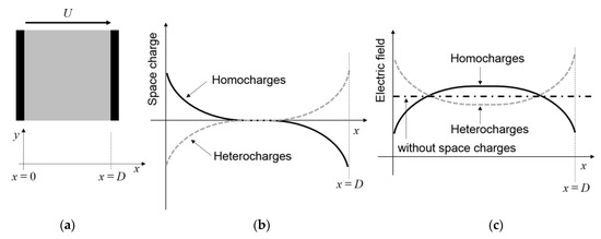
Figure 3.
(a) Insulation material with thickness D between two planar electrodes with applied voltage U; (b) schematic homocharge and heterocharge distribution; (c) effect of the charge distribution on the resulting electric field [2,8].
Homocharges are injected charges that are trapped close to the electrode, if charge injection exceeds the drift [2,37]. The presence of some impurities, e.g., cumyl alcohol, a byproduct of the XLPE crosslinking agent dicumyl peroxide (DCP), increase the trap density near the electrodes and supports the accumulation of homocharges [38].
Heterocharges are formed with and without a temperature gradient. In the absence of a temperature gradient, heterocharge accumulation results from the ionization of impurities. A spatial varying distribution of permanent dipole molecules form an inhomogeneous polarization and, thus, heterocharges [36,39]. Charges that have dissociated from molecules move to the electrodes and may also form heterocharges. With a temperature gradient, charges are injected at the high temperature electrode and move to the low temperature electrode, where they might not be extracted [2,40,41].
Surface charges at both electrodes are the result of the polarization of the material under an applied electric field and the presence of bulk space charges [40].
Injected charges may also form charge packets (charge pulses) that move to the opposite electrode. Measured charge packets are mainly found in polymeric insulation materials [42,43]. A description of the physics of charge pulses is reviewed in [43]. According to [44], charge packets are observable at electric fields of 10–50 kV/mm. At electric fields of >40 kV/mm a repetitive injection of charges is seen and several pulses move through the insulation. In [42], measured charge packets are divided into “fast” and “slow” packets. Fast charge packets have a mobility of up to 10−10 m2/(Vs) and a density of 0.07–0.1 C/m3. By contrast, slow charge packets have a mobility of 10−16–10−14 m2/(Vs) with a density >0.1 C/m3 [45]. The semicon interface between the polymeric insulation and the electrode shows a blocking behavior for charge packets, resulting in the accumulation of heterocharges and in a decrease of the lifetime [42,46].
4. Numerical Simulation of Charge Transport and the Electric Field in Direct Current (DC) Cable Insulations
Numerical simulations are a powerful tool to determine the charge transport and the corresponding electric field distribution within the insulation material and furthermore a complement to measurements. Two models are commonly described in literature to compute the charge transport and the electric field in DC insulations, where the corresponding equations are presented in Section 4.1 and the discretization with possible pseudo codes is shown in Section 4.2.
4.1. Equations to Simulate the Time-Varying Charge and Electric Field Distribution
The macroscopic description (“conductivity model”) of charge accumulation is based on the electric conductivity of the insulation and simulates an average value of positive and negative charge carriers (see e.g., [11,14]). The conduction is described at different temperatures and electric fields, but it does not describe the involved mechanisms (e.g., trapping or detrapping of charges). These mechanisms are modeled within the microscopic description (“bipolar-charge-transport- model”) [22,47].
The governing equations for the simulation, using the conductivity model, are the continuity equation, Poisson’s equation and Ohm’s law, i.e.,
with the current density inside the insulation , the magnitude of the electric field , the electric potential φ and the space charge density ρ [11,32]. Inserting (9) and (10) in (8), the electro-quasistatic field formulation:
is obtained [48,49,50]. The space charge oriented field formulation (8)–(10) and the scalar potential oriented field formulation (11) are approximations of Maxwell’s equations which holds under assumption that inductive effects can be neglected, i.e., [51].
For the simulation, using the bipolar-charge-transport-model, the continuity equation is extended by a “source-term” s and the electric conductivity is described by the charge density n and their mobility μ, i.e.,
where nμ is the density of mobile charge carriers, nt is the density of trapped charge carriers and κ = nμ∙μ is the definition of the electric conductivity. Charge generation results from injection processes that is described by the Schottky law [47,52,53,54,55]. Equal to the electric conductivity, the mobility is also a function of the temperature and the electric field [53,56]. Positive and negative trapped and mobile charge carriers have to be considered separately, resulting in 4 equations of the source-term:
where ne,μ is the density of negative mobile charges, nh,μ is the density of positive mobile charges (nμ = nh,μ + ne,μ), ne,t is the density of negative trapped charges and nh,t is the density of positive trapped charges (nt = nh,t + ne,t). The recombination coefficients are S0,1,2,3 and the trapping (detrapping) coefficients for positive and negative charges are Bh (Dh) and Be (De), respectively. The trap density for positive charges is nh,t,0 and for negative charges ne,t,0 [54]. To obtain the density of mobile charges, (12) is solved using the splitting method, which consists of first solving (12) with s = 0 and then solving s1 for mobile electrons and s2 for mobile holes in (15). For the density of trapped charges, only s3 for electrons and s4 for holes are evaluated [47].
Due to a temperature dependency of the conductivity and the mobility, the temperature distribution is computed by the heat conduction equation:
with the density of the insulation material δ, its specific heat capacity cp and thermal conductivity λ. The heat source is represented by [14].
4.2. Discretisation and Numerical Calculation Scheme
To use the bipolar-charge-transport-model several constants have to be determined. Furthermore, this model can only be solved with an explicit time integration. Alternatively to this, the conductivity model needs only 3 constants and can be solved with an explicit and an implicit time integration, where the implicit time integration can only be used for the scalar potential oriented field formulation (11). That makes, the conductivity model also applicable for complex HVDC cable components, like cable joints [57]. Thus, only the conductivity model is considered in the following.
Applying the finite integration technique (FIT) or the finite element method (FEM) to (8)–(10) results in a non-linearly coupled system of equations:
with the discrete divergence matrix GT, the vector of current densities j, the vector of electric dual cell charges q, the permittivity matrix Mε, the gradient matrix G, the vector of nodal scalar potentials Φ, the electric conductivity matrix Mκ, the vector of nodal temperatures uT and the boundary conditions for the electric problem b [58]. The discretization of (11) is:
showing that (17)–(19) and (20) are mathematically equivalent [58,59]. Applying an explicit Euler method to (20), the solution of Φ(tm+1) = Φm+1 is:
where m is the discrete time index and Δt is the time step length that has to be lower than ΔtCFL, determined by the Courant–Friedrich–Levy (CFL) criterion, for stability reasons [52]. Similarly as with (11), the time discretization of the heat conduction Equation (16), using an explicit Euler method, yields the update scheme:
where Mδ is the density matrix, Mc is the matrix of the specific heat capacity, Mλ is the thermal conductivity matrix, qT = Mκ(uT,Φ)GΦGΦ is the vector of heat sources and bT contains the boundary conditions for the thermal problem [48,49,60,61]. A possible calculation scheme to obtain the electric field and the space charge density, using (8)–(10), is depicted in Figure 4 and using (11) in Figure 5.
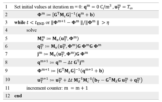
Figure 4.
Numerical computation scheme, to obtain the electric field and the space charge density, using the space charge-oriented field formulation (8)–(10) [11,58,59].
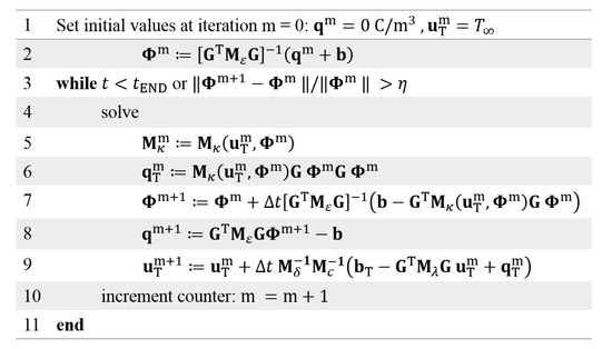
Figure 5.
Numerical computation scheme, to obtain the electric field and the space charge density, using the scalar potential field formulation (11) [11,58,59].
The computation starts with an assumed vanishing space charge distribution ρ = 0 C/m3 (q = 0) and a constant temperature equal to the environment temperature T∞. The vanishing space charge density results in a purely capacitive field that is determined by the permittivity and the geometry only. The time integration stops if a predefined time t = tEND or is obtained, where η 1 is the stop threshold and is the absolute value of the vector Φ at the discrete time step tm [11,58,59].
The simulation of an HVDC cable system includes the cable, the cable joint and the cable termination. From a numerical perspective, the cable joint and the cable termination are equally difficult to simulate. Both include different field-grading techniques and they consists of multiple subcomponents, resulting in interfaces between different dielectrics. Thus, the following simulations include cables and cable joints only.
5. Simulation of the Electric Field and the Space Charge Density within a Cable Insulation
Simulation results of a cable insulation are presented in this section, showing the behavior of the electric field and the space charge density under different thermal stress. In Section 5.1, the time-varying electric field is simulated and approximated, using the analytic solution of the stationary electric field. Furthermore, the stationary electric field and the corresponding charges are analyzed under different temperature gradients. The computation of the stationary electric field may result in instabilities during the iteration process, as shown in Section 5.2. Considering a varying environment of the cable, varying temperature and electric field distributions are computed and presented in Section 5.3.
5.1. Transient and Stationary Electric Field under Various Thermal Stresses
Several authors have studied space charge phenomena in DC power cables, after one of the first works of Lau in 1970. The space charge evolution in time has been described for the first time, using a non-linear electric conductivity, depending on the temperature only [62]. Within Eoll’s work in 1975, the stationary electric field is described, considering the dependency on the temperature and on the electric field and the losses within the insulation [30]. In [62] and [30] the electric conductivity is described by (6), where the expression is used in [62], due to a temperature dependency only. Equation (6) or the approximation (7) are also used in the following years (see e.g., [11,14,25,26,63,64]).
Considering a MI cable insulation, depicted in Figure 1b, the transient electric field stress and space charge distribution during the load of the cable is shown in Figure 6. The electric conductivity is given by (6) and the constants for the computation are summarized in Table 1. A convective heat flux is assumed at the outer sheath and described by
where αout is the heat transmission coefficient [65,66,67,68]. Using Figure 6, the maximum space charge density (Figure 6c) and thus, the maximum field inversion (Figure 6b) are obtained for a stationary temperature distribution, showing the maximum temperature gradient (Figure 6a).
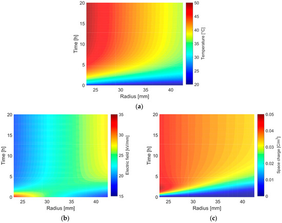
Figure 6.
(a) Transient temperature distribution within a MI insulation; (b) corresponding transient electric field stress; (c) corresponding transient space charge density.

Table 1.
Constants to simulate the transient electric field under load conditions in a MI cable insulation [11,30,65,66].
In [62], it is assumed that the thermal time constant is low in comparison to the electric time constant (1) and a stationary temperature is already obtained at t = 0 [64]. Thus, in several studies only the stationary temperature distribution is considered [11,14,25,26].
With (7), the stationary electric field is given in a closed analytic form. An analytic derivation of the stationary electric field and charge density starts from Gauss’ law (9), where Ohm’s law (10) is used to replace the electric field with the electric conductivity and the current density. Applying the chain rule and using the stationary current , one obtains:
With (24), a varying electric conductivity, either by a varying electric field and/or temperature or other processes will automatically result in accumulated charges [14,26]. For a radial symmetric electric field E(r), space charge ρ(r) and temperature profile T(r), (24) is reduced to:
With the Gauss law (9) to replace the charge density ρ(r) in (25) and an assumption of a constant permittivity (εr = const.), the stationary electric field is the solution of:
With the electric conductivity (7), the electric field is obtained by solving:
Considering negligible insulation losses and with constant parameters δ∙cp and λ, the stationary temperature is the solution of (16) for ∂/∂t = 0 [69] and is given by:
With (28), the solution of (27) is:
where C is a constant. Using the definition ab = exp(b∙ln(a)), (29) is reduced to:
With the applied voltage U, the constant C is:
In [3,62], the temperature is described by the thermal conductivity λ of the material and the heat losses of the conductor PV and is given by:
With (32) the electric field is:
Applying Gauss’ law, the corresponding stationary space charge distribution is:
Utilizing the stationary electric field E(r) and the initial electric field at t = 0 (E0(r) = U∙r−1∙ln(ra/ri)−1), a rough estimation of the transient electric field is obtained. With (11) and Figure 6b, a reasonable assumption for the time dependence of the transient electric field is an exponential function. The stationary electric field E(r) is equivalently given by (30) or (33), respectively. With an exponential approach and the time constant τ in (1), the transient electric field is:
With an electric field depending time constant, an approximation for τ is determined with the mean electric field U/(ra − ri). Using (7), the constants in Table 1 and the temperature distribution (28), with Ti = 50 °C and Ta = 35 °C, the numerically computed solution and the relative error of the approximation (35) are depicted in Figure 7. The relative error of (35) has the highest values in the vicinity of the conductor and the sheath, during the inversion of the field. The maximum error is about +13.58%. If the electric field approaches the stationary solution, the error decreases and is close to zero.
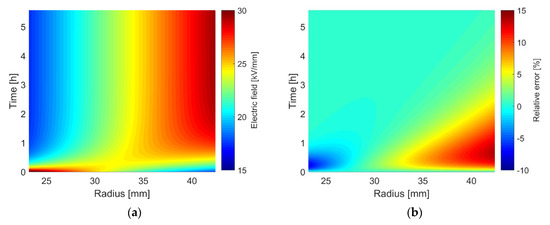
Figure 7.
(a) Numerically computed electric field distribution; (b) relative error between the numerically computed transient electric field and the approximation (35).
The stationary electric fields (30) within a MI insulation for a constant conductor temperature of Ti = 50 °C and a varying sheath temperature Ta are depicted in Figure 8 [11,22]. As depicted in Figure 8a, the inversion of the electric field is seen at temperature gradients higher than 5 °C. Temperature gradients higher than 20 °C result in a sheath electric field that is higher than the maximum electric field at t = 0, which is about 32 kV/mm. The space charge distribution in Figure 8b for a temperature gradient of ΔT = 0 °C results from the dependency of the conductivity on the electric field. At temperature gradients higher than 15 °C the charge density increases towards the sheath, resulting from the constant δE that is <−1 and the negative exponent of the radius r in (34).
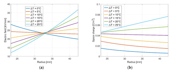
Figure 8.
(a) Stationary electric field within a MI insulation; (b) corresponding space charge distribution [11,22].
Within the insulation, a homogeneous electric field is desirable. To obtain a homogeneous electric field, δE needs to vanish, resulting in E(r) = U/(ra − ri). With (30), δE vanishes at a temperature gradient Ti − Ta = ln(ra/ri)/α ≈ 6 °C. Utilizing (33) this temperature gradient corresponds to losses of PV = 2πλ/α ≈ 10.5 W/m, with λMI = 0.167 W/(Km) [30]. With losses higher than 10.5 W/m, the field inversion increases and with lower losses the electric field is higher at the conductor in comparison to the field at the sheath [70]. The temperature coefficient α is approximately equal for XLPE and MI, but the thermal conductivity of XLPE is higher (λXLPE = 0.27–0.32 W/(Km)) in comparison to MI. Using an equal XLPE cable insulation, the losses are PV ≈ 17–20 W/m to obtain a homogeneous electric field. Thus, a better heat dissipation of XLPE results in higher transmitted power until the risk of high field values at the outer sheath occurs [5]. According to [25,26] the charge density is separated into two parts. One corresponds to the temperature dependency of the electric conductivity (ρT) and one corresponds to the electric field dependency (ρE). With a given temperature gradient both charge parts are of the opposite sign. With increasing field dependency (v) the effect of field inversion decreases, but the net charge density (|ρT| + |ρE|) increases. In comparison to MI, the electric field dependency of XLPE is 3.5 times higher [30,31]. Thus, the net charge density (|ρT| + |ρE|) is higher in polymeric cable insulations, whereby XLPE usually operate under lower applied electric fields [2,3].
5.2. Fast Calculation of the Steady State Charge Distribution
In the case of overvoltage (e.g., impulse voltage) or other effects, a transient simulation is mandatory. Under the assumption of no disturbances and a pure stationary electric field, the transient computation the field stress is often not necessary, because of the long operation time of power cables [1,11,25,26]. Thus, for the reliability of the insulation material it is sufficient to analyze the stationary electric field that is above the black dotted line in Figure 1a (∂/∂t ≈ 0). Excluding the conductivity model (7), the stationary electric field is not given in a closed analytic form. In addition to the explicit time integration of (8)–(10) or the explicit/implicit time integration of (11), the stationary electric potential is also obtained by a pseudo time stepping of the stationary current:
The corresponding charge distribution is obtained from Poisson’s Equation (9).
Using an explicit Euler method, the time step length Δt has to satisfy the CFL-criterion. With an implicit Euler method, there is no limit for Δt and the stationary electric field is theoretically obtained after the first iteration. Resulting from the rather low number of degrees of freedom, the explicit Euler method allows a fast computation of many time steps, while the benefit of the implicit method is reduced, because of solving a non-linear system. By using different acceleration techniques, the computation time, using an explicit Euler method, is further reduced, [60,61].
During the pseudo time stepping of (36), oscillations may occur, resulting from high electric field values and the non-linear electric conductivity. A diverging electric field is seen in Figure 9a, resulting from these oscillations [71]. A planar MI insulation with thickness D = 20 mm is considered. The electric conductivity is described by (6) and the conductivity constants are seen in Table 1. The conductor temperature Ti = 50 °C and the sheath temperature Ta = 35 °C. Using an applied voltage of 470 kV, oscillations at the sheath start to increase after 5 iterations. High electric field values result in increased conductivity values, having an effect on the computation of the electric potential φ in (36). Decreasing the voltage from 470 kV to 400 kV yields lower and converging field values (Figure 9b). Further possibilities to reduce the charge density and thus, the field strength are a lower temperature gradient and lower constants α and β [71].
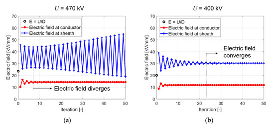
Figure 9.
Electric field at the conductor and the sheath in a 20 mm-thick MI insulation. (a) with an applied voltage of U = 470 kV, the electric field diverges after 5 iterations; (b) with a reduced voltage of U = 400 kV, the electric field converges [71].
Introducing an under-relaxation parameter ω, with ω [0, 1], the oscillations are minimized and the electric potential at the iteration step m + 1 is:
Using ω < 1, more iterations are required to obtain a stationary solution, but the result does not diverge. As depicted in Figure 10b, with U = 470 kV and ω = 0.95, the electric field after the first iteration is slightly reduced to 44.5 kV/mm and convergence is obtained after 30 iterations [71].
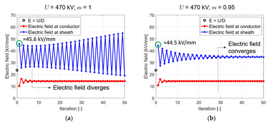
Figure 10.
Electric field at the conductor and the sheath in a 20 mm thick MI insulation. (a) with an applied voltage of U = 470 kV and ω = 1, the electric field diverges after 5 iterations; (b) with a voltage of U = 470 kV and ω = 0.95, the electric field converges [71].
A comparison between the explicit Euler time integration and the fixed point iteration, to obtain the measured stationary charge distribution in [72,73], shows a faster computation using the fixed point iteration. Depending on the electric field and spatial resolution, the fixed point iteration yields a faster computation of about one order of magnitude. High electric fields result in fast charge movements that need to be considered with a small time step, using the explicit time integration. This results in more time steps and a higher computation time until a stationary solution is obtained. Fast charge dynamics are neglected using the fixed point iteration, which yields a lower computation time [71].
5.3. Electric Fields in Power Cables, Considering the Environment
HVDC power cables are typically buried within the earth or the sea bed. The thermal conductivity of the insulation material and the environment have an effect on the resulting temperature gradient within the insulation and thus, on the operation current and voltage. The calculations of the thermal rating of power cables go back to the late 19th and early 20th centuries, due to the advent of electricity. Simplified formulas are derived to compute the temperature of the cable sheath and in the vicinity of the cable, by using analogous descriptions to electrostatic fields [74,75,76]. In [77,78], temperature gradients within the cable insulation and the sheath are also considered to obtain the conductor and sheath temperature. Furthermore, a humidity-dependent electric conductivity of the soil is used.
To obtain the stationary temperature distribution, (16) is solved with ∂/∂t = 0. Typically the density δ and the specific heat capacity cp of the insulation material or the soil are constant, but the thermal conductivity λ of soil or air depends on the humidity and on the temperature. A coupling between the thermal and the electric field results from the thermal heat source . As insulation losses have only a negligible influence on the resulting temperature distribution, the non-linear coupling can be reduced, resulting in a simplified temperature calculation [51,58,69].
A MI cable, buried 1.5 m, is considered and depicted in Figure 11 [77,78,79]. The electric conductivity is given by (6) and the necessary parameters are taken from Table 1, with rout = 52.4 mm and Ti = 55 °C.
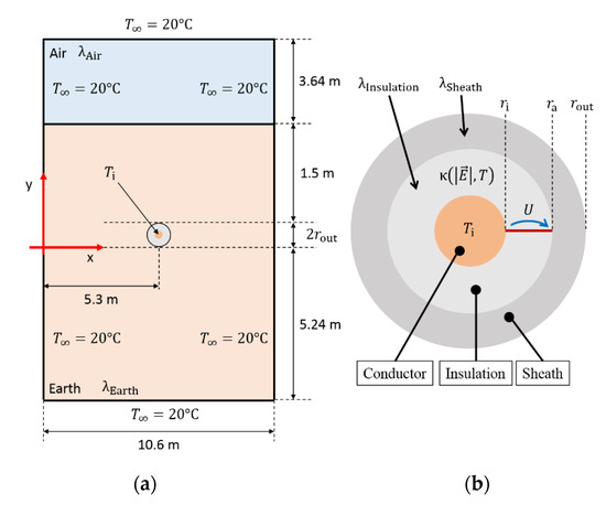
Figure 11.
(a) Two-dimensional geometry of a single cable within the earth; (b) the cable consists of conductor, insulating material and outer sheath [51].
Temperature-independent thermal conductivities of MI and the outer PE sheath are assumed with λMI = 0.167 W/(K∙m) and λPE = 0.3–0.4 W/(K∙m) [30,67,80]. Within the range of −30 °C and +90 °C, the thermal conductivity of air λAir depends on the temperature and is given by:
where T is the absolute temperature in Kelvin [51,67]. The thermal conductivity of soil is more complex to describe, but a good assumption is a dependency on the humidity only [77,78]. For moderate humidity values, the thermal conductivity attains values between 0.47 W/(K∙m) and 2.1 W(K∙m) and increases with increasing humidity [51,67]. Depending on the soil thermal conductivity, the temperature gradient within the insulation and the soil itself varies. This results in different temperatures at the earth–air interface (x = 5.3 m, y = 2rout + 1.5 m). For example, with a soil thermal conductivity of 0.47 W/(K∙m), the temperature at the earth–air interface is T = 32.4 °C and with 2.1 W/(K∙m), the temperature is reduced to T = 26.7 °C.
Within the insulation, an increased thermal conductivity results in an increased temperature gradient and, thus, in an increased field stress at the sheath (Figure 12). Due to the large distance of 1.5 m between the cable and the earth–air interface, the temperature distribution within the insulation is approximately radial symmetric. The temperature within the insulation and the outer sheath is depicted in Figure 12a. The vertical black dotted line shows the interface between the insulation and the outer sheath. The corresponding electric field is seen in Figure 12b.
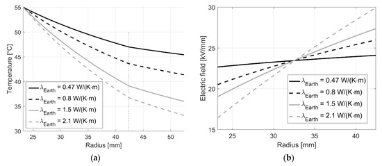
Figure 12.
(a) Simulated temperature distribution inside a MI insulation. The vertical block dotted line is the interface between the insulation and the outer sheath; (b) stationary electric fields stress, resulting from the temperature distribution [51].
The temperature gradient within the insulation increases from 8 °C (0.47 W/(K∙m)) to 18.3 °C (2.1 W/(K∙m)), resulting in a decreasing electric field at the conductor of 27.5% and an increasing field at the sheath of 24.2%. With a varying environment temperature (T∞), the effect on the insulation temperature also varies. With increasing T∞, the temperature gradient and the field stress at the outer sheath decreases. By contrast, the soil around the cable heats up and the temperature at the earth–air interface assumes its maximum value for dry soil (λ = 0.47 W/(K∙m)). With decreasing T∞, the effect on the environment is reduced, but the insulation is facing higher stress levels [51]. Considering a buried cable pair, a higher influence on the environment is seen, due to the additional heat losses of the second cable (see Figure 13).
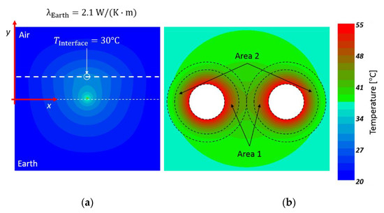
Figure 13.
(a) Temperature distribution around a MI cable pair, with a soil thermal conductivity of 2.1 W/(K∙m) and T∞ = 20 °C; (b) temperature distribution within the insulation [51].
The temperature of the earth–air interface increases of about 4 °C, compared to a single cable. Furthermore, the temperature distribution within the insulation is no longer radially symmetric, as seen in Figure 13b. Between both conductors (“Area 1”), the temperature is higher compared to “Area 2”, but the temperature gradient is higher in “Area 2”. Utilizing a metallic sheath between the insulation and the outer sheath, the temperature outside of the cable shows negligible changes, but results in an approximately radially symmetric temperature distribution within the insulation. Due to the high thermal conductivity of the metallic sheath in comparison to the insulation or the outer sheath, the non-symmetry of the temperature, seen in Figure 13b, is reduced. The temperature has approximately equal values at r = ra. The metallic sheath has a negligible influence on the environment and the temperature at the earth-air-interface remains unaffected. Thus, one-dimensional electric field simulations are also applicable for cable pairs, if a metallic sheath is considered.
The simulation results in Section 5 do not include the effects of interfaces, where charges accumulate due to a high trap density. These effects are modeled with an additional spatial variation, presented in the following section.
6. Simulation of Space Charge Effects at Interfaces and Surfaces and of Moving Charge Packets
The blocking behavior of interfaces is not considered in the commonly used conductivity models (3)–(7). The modeling of charges at interfaces is given in Section 6.1, where analytic and simulation results of the electric field in a cable and a dual-dielectric interface are shown. Using space charge measurements, an empirical conductivity equation, considering heterocharge accumulation in polymeric cable insulation, is developed in Section 6.2. In Section 6.3, the transient simulation of charge packets and a comparison to measurements are seen.
6.1. The Stationary Field Distribution, Considering Charges in the Vicinity of Electrodes and Dual-Dielectric Interfaces
6.1.1. Modeling of Charges Close to Electrodes
In [81,82], heterocharge build up at the electrodes is described with an extended conductivity equation, that has additional spatial variations towards the electrodes. A closed analytic description of the stationary electric field due to homo- or heterocharges at the electrodes within a cable insulation is shown in [70]. In [81], the additional spatial variations towards the electrodes are described with:
where fcon(r) yields spatial variations at the conductor (“con”) and fsh(r) at the sheath (“sh”). The conductivity increases or decreases by a factor of n towards the electrodes and ζ is a constant that defines the gradient of f(r). With (7), the total conductivity is:
Equal to (27), the electric field is the solution of:
describing the effects at both electrodes by the additional term f(r). Using the assumption fcon(r = ra) = 1 and fsh(r = ri) = 1, results in f (r) = fcon(r) at the conductor and f (r) = fsh(r) at the sheath. With the temperature distribution (28), the solution of (41) is:
Equal to (31), the constant K is computed with the applied voltage U and given by:
where
A comparison of (42) and (43) with (30) and (31) shows the additional term f(r) that is influenced by the electric field dependency only [70]. For example, the stationary electric field and charge distribution for ncon = nsh = 1.5 (ncon = nsh = 0.75), Ti = 50 °C, Ta = 35 °C, and ζcon = ζsh = (ra − ri)/10 are depicted in Figure 14 [11,22]. The conductivity of MI is described by (7) and the necessary constants are given in Table 1. Resulting from the negative exponent of f(r) in (42), n > 1 corresponds to a decreasing electric field and, thus, in additional accumulated homocharges and n < 1 describes additional heterocharges. With n = 1 additional homo- or heterocharge distributions vanish and bulk effects are only considered (see Figure 14b).
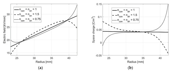
Figure 14.
(a) Example of the stationary electric field within a MI insulation, considering additional charge accumulation at both electrodes; (b) corresponding space charge distribution [70].
A heterocharge distribution affects the electric field at the sheath, while a homocharge distribution needs to be considered for the electric field at the conductor. Using a classical “line-commutated current source converter” (CSC) HVDC system, the direction of the current remains constant and the polarity of the applied voltage changes, to invert the direction of the power flow. This polarity reversal results in high electric field stress at the conductor, where the negative electric fields due to the space charges and the applied voltage are superimposed [2,4,83]. To avoid high field values, XLPE cables are used in modern “self-commutated voltage source converters” (VSC) HVDC systems [2,83].
6.1.2. Modeling of Charges Close to Interfaces of Different Dielectrics
Interfaces between two different dielectrics are found in cable joints and cable terminations. Accumulated interfacial charges are described by the Maxwell–Wagner–Sillars polarization, if constant permittivity and conductivity values are used within both dielectrics [14,84,85,86]. Due to the electric field depending on conductivity, the Maxwell–Wagner–Sillars model is not applicable [14,85]. Furthermore, space charges accumulate in the vicinity of interfaces, resulting from physical and chemical disorders and thus, a high trap density [14].
Space charge measurements within two dielectrics of XLPE (εr,XLPE = 2.3) and ethylene propylene rubber (EPR, εr,EPR = 2.9) are found in [84]. The applied voltage is U = 30 kV, the conductor radius is ri = 1.8 mm, with a temperature of Ti = 64 °C and the sheath radius is ra = 3.9 mm, with Ta = 42 °C. The interface radius is rInt = 3.25 mm. For the stationary temperature distribution, the thermal conductivity is λXLPE = 0.27 W/(K∙m) and λEPR = 0.3 W/(K∙m). The space charge distribution is obtained after t = 20,000 s [84,87]. For the electric conductivity, (7) is used, with the constants given in [14]. A sketch of the dual-dielectric-interface is seen in Figure 15a.
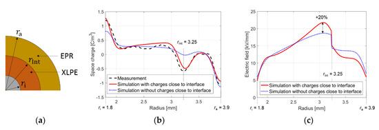
Figure 15.
(a) Sketch of the dual dielectric interface; (b) measured and simulated space charge distribution, with and without consideration of accumulated chares in the vicinity of the interface; (c) corresponding electric field of the simulated charge distribution [70,84].
To consider accumulated charges in the vicinity of interfaces, an additional conductivity gradient is applied [70]. Equal to the modelling of homo- and heterocharge in cables (39), accumulated charges close to the interface are described with:
where n and ζ have the equal meaning, compared to (39), but fXLPE is only valid for ri ≤ r ≤ rInt and fEPR is only valid for rInt ≤ r ≤ ra. The interfacial charges δInt are computed with:
with EEPR(rInt) being the electric field within the EPR material at the interface (r = rInt) and EXLPE(rInt) is the electric field in the XLPE material at the interface [84,86].
Measurements and simulation results with and without accumulated charges close to the interface are seen in Figure 15b, where the corresponding electric field is depicted in Figure 15c. The simulation results are obtained with (39) and (45) [70]:
The simulation results, considering charges close to the interface show fewer differences to the measurements, compared to the conductivity model (7). Furthermore, the accumulated charges in the vicinity of the interface (rInt = 3.25 mm) increase the electric field of 20%, highlighting the importance of accurate modelling of HVDC components with multiple subcomponents.
6.2. Empirical Conductivity Equation for the Simulation of Heterocharges in Polymeric Cable Insulations
A different approach to model the electric conductivity with additional spatial variations in the vicinity of the electrodes is described in [88,89,90]. The conductivity is given by:
where Kcon and Ksh yield conductivity variations at the conductor and the sheath. The constant rx defines the distance between the conductor (ri) and the position of the highest gradient (Kcon − Ksh = 0.5 at r = rx) and χ defines the gradient of Kcon and Ksh in the vicinity of both electrodes, which has an effect on the magnitude and the shape of the resulting heterocharge distribution [88,89]. Considering a planar insulation, ri = 0 and ra = D. To define the constants rx and χ, different measurements are taken from literature.
The empirical conductivity Equation (47) is valid for heterocharges only, because of considered low applied electric fields (<20 kV/mm) only [88,89]. Furthermore, measured heterocharges in XLPE and LDPE insulations, at an applied average electric field below 20 kV/mm, are found in [73,91,92,93]. For simplicity, χcon = χsh = χ is assumed. To obtain the constants rx and χ, a “conductivity gradient region” Δ is defined and yields rx = Δ/2 and 10χ ≈ Δ [88,89].
A common measurement technique is the pulsed electro acoustic (PEA) method, where surface charges and bulk space charges are subjected to a filtering process during the measurement, giving inaccurate results at the conductor and the sheath [15]. Thus, a Gaussian curve instead of a delta function is obtained, if a space charge free material under voltage load is measured [40,93,94,95]. An example of a space charge measurement within an XLPE cable insulation is seen in Figure 16, also indicating heterocharges and “filtered” surface charges at both electrodes [73].
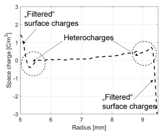
Figure 16.
Example of a space charge measurement within an XLPE cable insulation. “Filtered” surface charges appear as a Gaussian curve [73].
For an accurate comparison between simulated space charges and a measured charge distribution, surface charges at both electrodes need to be considered. Surface charges at the conductor δ+ and the sheath δ− are derived from [40] and approximately described by:
for a cylindrical geometry. Induced charges, resulting from accumulated space charges, represent the first term on the right-hand side in (48). The second term represents the capacitance charges induced by the polarization of the material under an applied voltage. To combine the surface charges and the bulk space charge, δ+ and δ− are divided by the spatial discretization Δh [96]. Finally, to compare simulations and measurements, the simulation results need to be converted to an equivalent signal, using a Gaussian filter [40].
For the calibration of the filter, the space charge density vanishes within the bulk. The voltage is applied for a short period of time, to compare the space charge measurements and simulation results at t ≈ 0 s, for example seen in Figure 17 [95,97]. The black dashed line are the measurements, the black line is the unfiltered simulation result and the red line is the filtered simulation result. With no bulk space charges, (48) is reduced to δ+ = ε0εrE(ri) and δ− = ε0εrE(ra) [97]. In Figure 17, the applied voltage is U = 90 kV, ri = 4.5 mm, ra = 9 mm and εr = 2.3 [14].
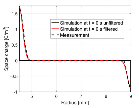
Figure 17.
Comparison of measurements against filtered and unfiltered simulation results at t ≈ 0 s. [14,95].
Several space charge measurements within a planar and a cylindrical insulation material of XLPE and LDPE are seen in [72,73,91,93]. By minimizing the difference between the simulated filtered space charge distribution and the measured charge distribution, the constants for rx = Δ/2, 10χ ≈ Δ and Δ are summarized in Table 2. The measurements in [91] and the corresponding simulations are for example seen in Figure 18. To describe the electric conductivity of XLPE and LDPE, (4) is used, where the constants are given in [14,56,89,98,99].
Table 2.
Distance constant χ and position rx for the simulation of space charge measurements in [72,73,91,93]. The absolute value of the applied voltage is |U| = 20 kV.
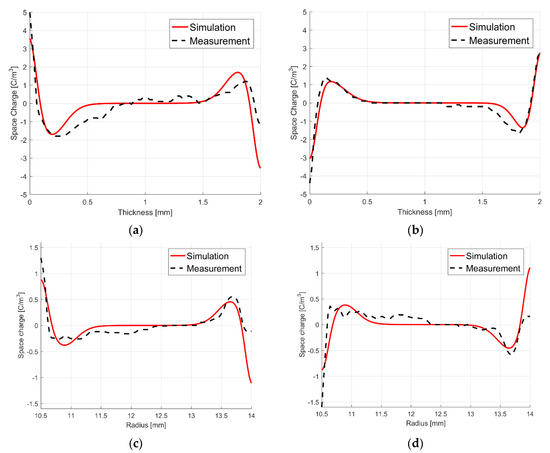
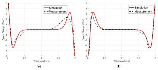
Figure 18.
Measured and simulated charge distribution in a XLPE and a LDPE insulation [91]. (a) XLPE, planar, +U; (b) XLPE, planar, −U; (c) XLPE, cylindrical, +U; (d) XLPE, cylindrical, −U; (e) LDPE, planar, +U; (f) LDPE, planar, −U. The absolute value of the applied voltage is |U| = 20 kV.
The constants χ and rx in (47) are approximated with χ = (0.25∙D)/10 and rx = (0.25∙D)/2 for a planar insulation and with χ = (0.25∙(ra − ri))/10 and rx = (0.25∙(ra − ri))/2 for a cylindrical insulation [88,89]. Utilizing a constant applied voltage with positive and negative polarity, the polarity of the charge density also changes, but the magnitude and the shape remains unaffected. This is called the “mirror image effect” and seen in Figure 18a–f. The effect is discussed in [97], where possible explanations are a spatially varying polarization of the dielectric and the injection of charges at the electrodes [100,101].
Accumulated heterocharges are approximately seen in one quarter of the insulation thickness, independent of the insulation material or the thickness. One possible assumption for accumulated heterocharges within this region might be the resolution of the measurement technique. On the other hand, the PEA method has a resolution of 1.6 μm for a one dimensional planar insulation with a thickness of 25–27,000 μm and 0.1–1 mm for a cable insulation with a thickness of 3.5–20 mm [94]. Thus, the resolution is accurate enough to separate between heterocharges and bulk space charges.
Differences between the simulations and the measurements in Figure 18 may come from the constants to describe (4) or the approximate description of the surface charges in (48). The electric conductivity of polymeric insulation materials differs with the preparation, which affects the constants of the conductivity models (3)–(7). Conductivity measurements of XLPE, taken from several references, are depicted e.g., in [95]. The measurements differ of about one order of magnitude and consequently different constants are obtained, when using the same conductivity model (4). The distribution of a measured space charge density shows a dependency on many factors, e.g., the electric conductivity, the local electric field or the electrode material. Consequently, it is very difficult to simulate the charge distribution of different references with a unique conductivity model, even if it is the same material [95,102,103]. Differences between a simulated and a measured space charge distribution are minimized, if conductivity and space charge measurements of the material are provided. Then, an error that might occur due to the use of conductivity measurements of different references, is reduced.
6.3. Transient Simulation of Charge Packets within a Cross-Linked Polyethylene (XLPE) Cable Insulation
Space charge and conductivity measurements of a medium voltage (MV) XLPE cable are given in [14]. These measurements show space charges, moving from the conductor to the sheath and a buildup of heterocharges (see Figure 19l). In addition to a varying conductivity, space charges accumulate due to a varying permittivity as well (see (24)). Analogously to [81] the permittivity is described by:
where ncon,ε and nsh,ε are the increasing factors at the conductor (“con”) and the sheath (“sh”) and ζcon,ε and ζsh,ε are constants defining the gradient of εr(r) at both electrodes. The constant bulk permittivity is εr,Bulk. A reasonable modelling approach for moving charges is an electric conductivity, having the shape of a Gaussian pulse and moving through the insulation [45,95]. With the non-linear bulk electric conductivity the total electric conductivity is:
where ncon,κ and nsh,κ are the increasing factors, ζcon,κ and ζsh,κ constants for the shape of the pulse and vκ is the velocity of the Gauss pulse (velocity of the moving charge pulse). The constants for the simulation results are summarized in Table 3. The cylindrical geometry has a conductor radius of ri = 4.5 mm, a sheath radius of ra = 9 mm and a bulk permittivity of εr,Bulk = 2.25. A time-independent temperature distribution is used and described by (28). For the bulk electric conductivity, the hopping model (4) is used, with the constants EA,2 = 1.48 eV, K2 = 1∙1014 A/m2 and γ2 = 2 × 10⁻⁷ m/V [14,81]. A comparison between the measurements and the simulation results, at the time t = 0 s, t = 10.000 s and t = 20.000 s, is seen in Figure 19. The results are obtained along the red evaluation line in Figure 1b.
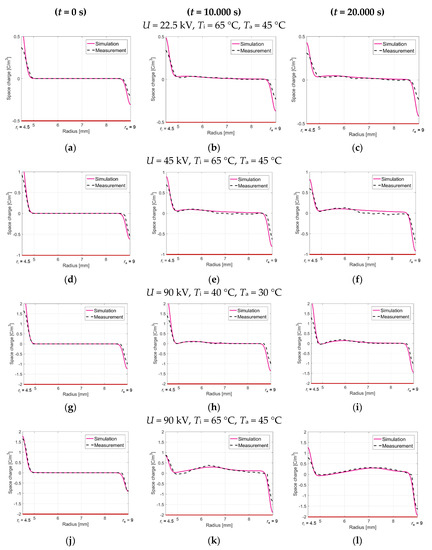
Figure 19.
Comparison between a measured (dashed line) and simulated (solid line) space charge distribution within a medium voltage (MV) XLPE cable insulation. (a) t = 0 s, U = 22.5 kV; (b) t = 10,000 s, U = 22.5 kV; (c) t = 20,000 s, U = 22.5 kV; (d) t = 0 s, U = 45 kV; (e) t = 10,000 s, U = 45 kV; (f) t = 20,000 s, U = 45 kV; (g) t = 0 s, U = 90 kV, Ti = 40 °C, Ta = 30 °C; (h) t = 10,000 s, U = 90 kV, Ti = 40 °C, Ta = 30 °C; (i) t = 20,000 s, U = 90 kV, Ti = 40 °C, Ta = 30 °C; (j) t = 0 s, U = 90 kV, Ti = 65 °C, Ta = 45 °C; (k) t = 10,000 s, U = 90 kV, Ti = 65 °C, Ta = 45 °C; (l) t = 20,000 s, U = 90 kV, Ti = 65 °C, Ta = 45 °C [14,95].
Table 3.
Characteristic values for (49) and (50), for each applied voltage and temperature gradient [14,95].
The used constants in Table 3 yield the best fit between the measurements in [14] and the simulation results. Increasing factors nsh,ε = nsh,κ = 1 indicate no increase/decrease of the permittivity and conductivity, which makes the corresponding constants ζsh,ε and ζsh,κ unnecessary. The conductivity factor ncon,κ increases with voltage and temperature, where possible reasons are detrapped charges and thermally activated and electric field assisted injection [20].
Characteristics for a charge packet are reported in [20]. Charge packets have to include:
- the formation of space charge regions,
- moving regions,
- a shape that is approximately maintained during motion,
- a periodic process (repetitive injection).
The simulation results in Figure 19 show space charge regions moving through the insulation that are especially seen in Figure 19k,l (I), (II). During the motion, the charge pulse slightly changes shape (III), but a periodic repetition (IV) is not seen. In [42], a repetitive injection of charge packets is seen at electric fields >40 kV/mm, whereas the electric fields in the simulations are between 5 kV/mm and 30 kV/mm.
The results in Figure 19 show only positive charges moving from the conductor electrode to the sheath, which conforms with results in [24,43]. The simulated charge packet drift with a velocity of vκ = 3 × 10⁻⁸–7.5 × 10⁻⁸ m/s, depending on the temperature and the electric field. With a mean electric field of E = U/(ra − ri) these velocity values correspond to mobility values (μ = vκ/E) of μ = 6 × 10⁻¹⁵ m2/(Vs) (a), 3 × 10⁻¹⁵ m2/(Vs) (b), 2.5 × 10⁻¹⁵ m2/(Vs) (c) and 3.75 × 10⁻¹⁵ m2/(Vs) (d). The mobility values are about 10−15 m2/(Vs), which characterize them as “slow” charge packets [45].
A comparison between the simulated charge density and the measurements is depicted in Figure 19 and shows a good agreement with the ocular norm. For the reliability of the cable insulation, the electric field needs to be determined. Thus, the mean difference between the simulated and the measured electric field is shown in Table 4. The mean difference lies between 1% and 22%. For example a mean difference between the filtered simulation results and the measurements of 12.5% (Figure 19l) is depicted in Figure 20. In comparison to the conductivity model in [14], the mean differences are in the same range in (a) and (b) and below the values of [14] in (c) and (d). With (49) and (50), one possibility of high values in Table 4 are the filtered surface charges at both electrodes. The approximation in (48), together with the filtering process, yields the highest differences at both electrodes, while within the bulk, the differences remain low (see Figure 18 and Figure 19).
Table 4.
Mean difference between the simulated and the measured electric field, using (49) and (50) and the results in [14,95].
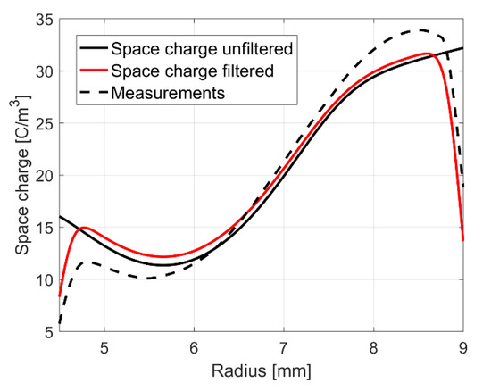
Figure 20.
Corresponding electric field of the filtered and unfiltered simulation results in Figure 19l, compared with measurements at the moment t ≈ 20,000 s. [95].
Compared to the unfiltered simulation results in Figure 20, the measurements show lower values at both electrodes, due to the filtering process of the measurement technique. The surface charges and the bulk space charges are “mixed” yielding a Gaussian-like shape at both electrodes (see Figure 16). During the simulation, these mixed charges result in a reduction to the electric field and can be misinterpreted as only being homocharges (see Figure 19 and Figure 20). Compared to the maximum initial electric field of 28.85 kV/mm, the unfiltered electric field at t = 20,000 s is about 32 kV/mm (increase of 11%). The electric field at the sheath is further increasing due to the charge pulse moving closer to the sheath, resulting in the accumulation of heterocharges (see Figure 14) [42]. A comparison between the different conductivity models in Section 5 and Section 6 is depicted in Table 5.
Table 5.
Comparison of different conductivity models and their description of space charge accumulation within the insulation.
Commonly used in literature are the conductivity models, represented in the Equations (3)–(7). Space charge accumulation and electric field variations within the insulation, resulting from temperature and electric field changes, are described. The stationary electric field is given in a closed analytic form. The electric field is connected to the applied temperature gradient, but only a mean charge density of one sign is computed. Effects at interfaces and surfaces are neglected. Such effects are described with additional spatial variations, e.g., (39) or (45) and (40), but the necessary constants are difficult to determine. Using (47), the additional constants to describe effects in the vicinity of the electrodes are evaluated with space charge measurements. By contrast, (47) is limited to heterocharges only and, equal to (39) or (45) and (40), only valid for the stationary case. Transient processes are simulated with (49) and (50), where additional spatial variations move within the insulation. The models (49) and (50) reduce the difference between simulation and measurement, but the additional constants vary over time and are determined by measurements.
The insulation materials in Section 5 and Section 6 are considered without defects. It is often difficult to determine the defects and their electrical and thermal material characteristics. Commonly, an air-filled void with a vanishing electric conductivity (κVoid = 0), in the absence of partial discharges (PD), is assumed [104,105,106].
7. Accuracy of the Electric Field Computation within Cables and Cable Joints
Compared to the scalar potential field formulation (Figure 5), the space charge-oriented field formulation in Figure 4 uses an additional averaging process to compute the charge density. Utilizing the cable geometry in Table 1 and the conductivity model (7) to describe a MI insulation, the analytic solution of the stationary electric field is given by (30), where Ti = 50 °C and Ta = 35 °C [11,59]. The analytic solution, together with the simulation results, using Figure 4 and Figure 5 are depicted in Figure 21a. Both formulations show a good accuracy in the ocular norm. Utilizing the space charge-oriented field formulation (8)–(10), inaccurate results are especially seen at the conductor, while using (11) the error has its maximum value at the sheath (see Figure 21b). With (8)–(10), the maximum error is 0.723%, with an average error of 0.3%. With (11), the maximum error (0.677%) and the average error (0.25%) are slightly lower. Equal to the results in Section 5.2, high electric field values are obtained during the time integration, resulting in inaccurate field values. Increasing the stationary electric field by decreasing the field dependency v (see (30)), the maximum error at the conductor is >1.5% using (8)–(10), but utilizing (11), the maximum error at the sheath has only slightly increased (0.74%) [59].
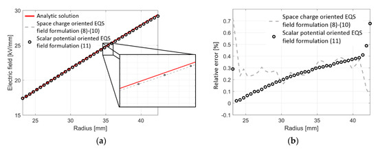
Figure 21.
(a) Stationary electric field, computed with (8)–(11), together with the analytic solution; (b) relative error between both formulations and the analytic solution [59].
Cable joints and terminations are geometrically more complex than cable insulations, due to different dielectric materials and the resulting interfaces. Resulting from these interfaces and other factors it is widely believed that cable joints and terminations are the least reliable components of a HVDC cable system [4,84]. Furthermore, the use of field-grading materials (FGM), results in difficulties while simulating such components. Such materials have a strongly non-linear dependency on the electric field and a lower dependency on the temperature [107,108]. In [107], the electric conductivity is given by:
where the constants are κ0,FGM = 7 × 10⁻¹¹ S/m, E1 = 1.23 kV/mm, E2 = 2.23 kV/mm, N1 = 1, N2 = 0.35, mFGM = 5.7 × 10⁻⁶ m/V and m0 = 2.15 × 10⁻⁶ m/V. In (51), the temperature dependency is neglected for simplicity. With field values <1 kV/mm, the material is nearly an insulator with an electric conductivity of 10−10 S/m–10−8 S/m. Between 1 kV/mm and 2.5 kV/mm, the electric conductivity increases of about six orders of magnitude. At fields >2.5 kV/mm, the electric conductivity is nearly constant and approximately 10−2 S/m. Due to the large variety of the conductivity values, the time constant (1) lies between 0.89 s and 8.9 × 10⁻⁹ s, with a relative permittivity of the FGM εr,FGM = 10 [59,109].
The geometry of the simulated cable joint is depicted in Figure 22a [59,109]. The simulation time tEND = 2 μs, with a time step of Δt = 0.0133 μs, yields a relative difference of between the discrete time steps m and m + 1. For simplicity and due to the short time tEND, the electric conductivity of XLPE and insulating silicone rubber (LSR) are assumed to be constant and given by κXLPE = 10−15 S/m and κLSR = 5 × 10⁻¹³ S/m. The relative permittivity of both materials is εr,XLPE = 2.3 and εr,LSR = 3.5 [59,109].
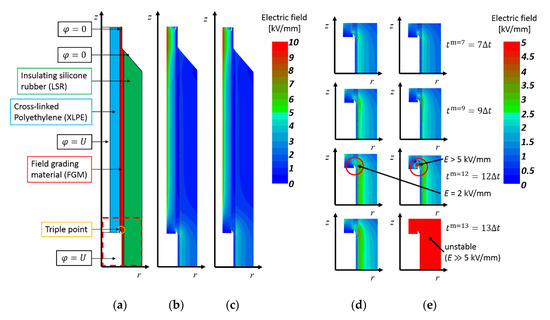
Figure 22.
(a) Geometry of cable joint, using field grading materials; (b) initial electric field; (c) stationary electric field, computed with (11); (d) electric field, computed with (11) at the time t = tn, with n = 7, 9, 12 and 13; (e) electric field, computed with (8)–(10) at the time t = tn, with n = 7, 9, 12 and 13. Inaccurate electric field values are seen after n = 12 [59,109].
In Figure 22b,c, the initial electric field (t = 0 s) and the stationary electric field are seen. Especially in the vicinity of the triple point, the field-grading material reduces the electric field stress. The stationary field distribution in Figure 22c is computed using the scalar potential field formulating (11), while the space charge formulation (8)–(10) yields unstable results at tm=13 = 13Δt, as seen in Figure 22d,e.
High electric field values occur in the vicinity of the triple point. The sharp edge in the cable joint geometry results in a compression of the potential lines and thus, in a high potential gradient. Using (8)–(10), electric field values >5 kV/mm are simulated at tm=12 = 12Δt and the electric conductivity has values of 10−2 S/m (Figure 22e). Consequently, the chosen time step size yields unstable field values. Stable field values are computed with (8)–(10), if the time step size is reduced to Δt = 0.0066 μs. With (11), an averaging process is needed to compute the electric field = −grad(φ). With (8)–(10), an additional averaging process is needed to compute the charge density (see (8)). Due to the additional averaging process and the non-linear electric conductivity, unstable electric field values are delivered [59].
8. The Electric Field of Ground Electrodes, Considering the Effect of Electro-Osmosis
A special case of an electro-quasistatic field is seen in the vicinity of HVDC ground electrodes, where the time varying electric field is the result of a drying process of the soil and its humidity dependency. A short overview of the computation is given in this section.
Common system configurations of HVDC transmission are monopole or bipole [83,110,111]. To use the earth or the sea for the return current, ground electrodes within the earth or on the sea bed are installed. Such electrodes are placed in different depths to ensure high conductivity values and are surrounded by a coke bed to reduce electrolytic corrosion and thus, the loss of electrode material [110,112].
Under the influence of the resulting electric field of ground electrodes buried within the earth, the water around the anode drift away and the soil around the electrode dries out due to the effect of electro-osmosis [110,112]. Electro-osmosis needs to be avoided due to a decrease of the electric conductivity and an increase of the electric field and the surface step voltage. To prevent soil from drying, some HVDC projects have arrangements to add water, if the soil moisture concentration falls below a certain value [110].
Resulting from the electric conductivity of earth that depends on the humidity and the temperature distribution, the electric field varies both in space and time, respectively. This special case of an electro-quasistatic field, shows no accumulated space charge and results from an electric conductivity that depends on a varying humidity concentration.
Water-saturated soil behaves as an electrolyte, where charges are injected into the soil if electrodes are connected. If the charges move under an applied electric field, they carry water molecules by exerting a viscous drag on the water around them. Due to more mobile positive charges than negative ones, there is a net water flow from the anode to the cathode [113,114,115]. The continuity equation of water flow describes the time-varying humidity concentration (volumetric water content) θ with:
where is the water flow [116,117]. Darcy’s law describes the water flow under the influence of an applied electric field with:
where k is the electro-osmotic hydraulic conductivity (also called “electro-osmotic conductivity” or “electro-osmotic permeability”). Due to the constant current of an HVDC system, the electric potential φ and the electric field are the solution of the stationary current problem (36). With losses within the conductor and the soil, the temperature is evaluated from (16).
The electric conductivity of soil is difficult to determine due to the dependency on several factors like the humidity, the temperature distribution, the composition and the size of silt, clay and sand particles. From [118,119], the electric conductivity is approximately correlated to the humidity and has a low temperature dependence. Using measurements from [120,121,122,123,124], the electric conductivity is described with the model:
where the constants are κ0,θ = 2.5 × 10⁻¹ S/m, bθ = 1.5 and κs = 2 × 10⁻⁵ S/m [117]. To consider the temperature dependency, (54) is extended by a correction factor g(T) and finally given by:
with the absolute temperature in kelvin [119]. Measurements in [113,114,125] show the electro-osmotic conductivity with a humidity dependency only. Due to no water flow for a vanishing electro-osmotic conductivity, k is described by:
The constants are k0,θ = 8.5 × 10⁻⁹ m2/(Vs) and aθ = 1.4. Heat losses within the conductor of the ground electrode and within the soil result in a temperature increase where the thermal conductivity decreases with decreasing humidity [89]. Additionally, the thermal conductivity shows a dependency on the temperature over a temperature range of 2 °C–92 °C in [126]. Measurements of the thermal conductivity λ in [77] and [126] are approximated by:
with the temperature dependent variables αθ = −0.024∙(T-273.15) + 3.049, βθ = 0.067∙(T-273.15) + 13.867 and γθ = 6.67 × 10⁻⁴∙(T-273.15) + 0.299. The measurements of the soil electric conductivity, electro- osmotic conductivity and thermal conductivity, together with their corresponding models (55)–(57) are seen in Figure 23 [127].
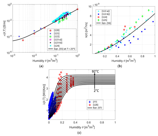
Figure 23.
(a) Measurements of the electric conductivity of soil and fit by (55) at a temperature of 25 °C; (b) measurements of the electro-osmotic conductivity of soil and fit by (56); (c) measurements of the thermal conductivity of soil and fit by (57) [77,113,114,120,121,122,123,124,126,127,128].
The electro-osmotic conductivity is in the range of 10−9 m2/(Vs). The effect of thermo-osmosis, due to a temperature gradient, is equally described as (53). By contrast, the thermo-osmotic conductivity is about 3 orders of magnitude lower than k and can be neglected in HVDC applications [128].
The time-varying humidity θ, the electric scalar potential φ and consequently the electric field are computed within a coupled electro-thermal-electro-osmotic simulation of (16), (36), (52) and (53). The coupled problem can only be solved with an explicit time integration, where Figure 24 shows a possible pseudo code. Equal to Figure 4 and Figure 5, the computation stops if a predefined time t = tEND or , where η 1 is the stop threshold, are obtained. Compared to the thermal problem, the time constant of the transient electro-osmosis process is higher [129]. Thus, humidity variations immediately affect the thermal conductivity and the temperature, resulting in a weak coupling between the quantities θ and T in Figure 24 [127].
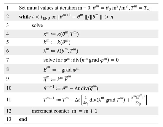
Figure 24.
Pseudo code to obtain the time-varying humidity concentration (θ), the temperature (T) and the electric field () [128].
Simulation results in [127] indicate electro-osmosis, with time constants up to years. Thus, it is only considered in the close vicinity of the electrode [129]. High electric field values also increase the surface step voltage right at the electrode. For short operation times of a few days, electro-osmosis might be omitted within the model, used for the computation of the surface step voltage, as its effects are negligible.
9. Conclusions and Outlook
This review showed the advances in the calculation and simulation of HVDC cables in the past few years. With an overview of the charge transport in commonly used insulation materials, a description of the conductivity models in use and the tools necessary to simulate HVDC cable components, with or without consideration of the environment, were presented. Finally, results of the charge and electric field behavior in HVDC cable insulations were shown and compared against analytic solutions and measurements.
Utilizing a conductivity-based cable model, the space charge-oriented field formulation and the scalar potential oriented field formulation were able to compute the time-varying electro-quasistatic field and space charge distribution within the insulation. Different models were found in literature to describe the non-linear electric conductivity and considered bulk effects only. These models were able to describe e.g., the “mirror image effect” or the effect of “field inversion”. The conductivity and the permittivity models were extended to consider effects at interfaces and surfaces and to model moving charge packets. Utilizing the extended models, differences between simulations and measurements were reduced, compared to commonly used models. Furthermore, a stationary heterocharge distribution was found to accumulate in 25% of the insulation thickness, independent of the insulation material.
Fast charge movements were considered with a low time step length during the time integration, using an explicit Euler method. To reduce the computation time, pseudo time stepping of the stationary current was applied, where oscillations were reduced with under-relaxation techniques.
Compared to the scalar potential formulation, the space charge formulation showed a lower accuracy, when computing complex geometries or materials with a strongly non-linear electric conductivity. The space charge formulation yielded unstable field values, due to an additional averaging process, when computing the charge density.
The electric field of HVDC ground electrodes is a special case of an electro-quasistatic field. Due to the effect of electro-osmosis, the electric conductivity and the electric field within soil varies in time, resulting from the constant current. Electro-osmosis is a slow process and needs to be considered only in the close vicinity of the electrode.
A description of charge dynamics in unmodified, and modified insulation materials are still part of ongoing research. Modified insulations consist of polymeric materials with added nano-dielectrics that show an influence on the temperature and electric field dependency and consequently on the charge distribution within the bulk and at interfaces. Another area of research includes liquid insulation materials, e.g., transformer oil, where the drift and the diffusion of charges need to be considered. Conductivity models are not applicable to describe both. The bipolar charge-transport model may describe drift and diffusion, but needs to be improved or simplified, making it usable for complex geometries.
Author Contributions
Conceptualization, C.J. and M.C.; Methodology, C.J. and M.C.; Software, C.J.; Validation, C.J.; Formal Analysis, C.J. and M.C.; Investigation, C.J. and M.C.; Resources, C.J. and M.C.; Data Curation, C.J. and M.C.; Writing-Original Draft Preparation, C.J. and M.C.; Writing-Review and Editing, C.J. and M.C.; Visualization, C.J. and M.C.; Supervision, M.C.; Project Administration, M.C.; Funding Acquisition, M.C. All authors have read and agreed to the published version of the manuscript.
Funding
This work was supported by the Deutsche Forschungsgemeinschaft (DFG) under the grant number CL143/17-1.
Conflicts of Interest
The authors declare no conflict of interest.
Nomenclature
| Capital letters | |
| Bh | Trapping coefficient for positive charges [1/s] |
| Be | Trapping coefficient for negative charges [1/s] |
| D | Thickness of a planar insulation [m] |
| Dh | Detrapping coefficient for positive charges [1/s] |
| De | Detrapping coefficient for positive charges [1/s] |
| Electric field [V/m] | |
| E0(r) | Electric field within a cable insulation at t = 0 [V/m] |
| E1 | Constant for the electric conductivity of FGM in (51) [V/m] |
| E2 | Constant for the electric conductivity of FGM in (51) [V/m] |
| EA,1 | Activation energy in (3) [eV] |
| EA,2 | Activation energy in (4) [eV] |
| EA,3 | Activation energy in (5) [eV] |
| Ee | Energy of charge carriers within the band diagram [eV] |
| ERef | Reference electric field in (7) [V/m] |
| ETrap | Trap depth [eV] |
| G | Discrete gradient matrix |
| GT | Discrete divergence matrix |
| I | Current [A] |
| Current density [A/m2] | |
| K1 | Conductivity constant in (3) [A/m2] |
| K2 | Conductivity constant in (4) [A/m2] |
| K3 | Conductivity constant in (5) [S/m] |
| Kcon | Conductivity variations in the vicinity of the conductor in (47) |
| Ksh | Conductivity variations in the vicinity of the sheath in (47) |
| Mc | Discrete matrix of the specific heat capacity |
| Mδ | Discrete density matrix |
| Mε | Discrete permittivity matrix |
| Mκ | Discrete electric conductivity matrix |
| Mλ | Discrete thermal conductivity matrix |
| N1 | Constant for the electric conductivity of FGM in (51) |
| N2 | Constant for the electric conductivity of FGM in (51) |
| PV | Losses per length within the conductor [W/m] |
| S0,1,2,3 | The recombination coefficients for different charge types [m3/(As∙s)] |
| T | Temperature [°C] |
| Ta | Sheath temperature [°C] |
| Ti | Conductor temperature [°C] |
| T∞ | Environment temperature [°C] |
| U | Voltage [V] |
| W | Mean band gab energy [eV] |
| Small letters | |
| aθ | Constant for the electro-osmotic hydraulic conductivity of soil in (56) |
| bθ | Constant for the electric conductivity of soil in (54) |
| b | Boundary conditions for the electric problem |
| bT | Boundary conditions for the thermal problem |
| cp | Specific heat capacity [W∙s/(kg∙K)] |
| hP = 6.626∙10−34 | Plank constant [J∙s] |
| j | Vector of current densities |
| k | Electro-osmotic hydraulic conductivity [m2/(Vs)] |
| k0,θ | Constant for the electro-osmotic hydraulic conductivity of soil in (56) |
| kB = 1.38∙10−23 | Boltzmann constant [J/K] |
| m | Discrete time index |
| m0 | Constant for the electric conductivity of FGM in (51) [m/V] |
| mFGM | Constant for the electric conductivity of FGM in (51) [m/V] |
| ncon | Conductivity increasing/decreasing factor at the conductor in (39) |
| ncon,ε | Conductivity increasing/decreasing factor at the conductor in (49) |
| ncon,κ | Conductivity increasing/decreasing factor at the conductor in (50) |
| nEPR | Conductivity increasing/decreasing factor in (45) |
| ne,t | Density of negative trapped charges [As/m3] |
| nh,t | Density of positive trapped charges [As/m3] |
| ne,μ | Density of negative mobile charges [As/m3] |
| nh,μ | Density of positive mobile charges [As/m3] |
| ne,t,0 | Trap density for negative charges [As/m3] |
| nh,t,0 | Trap density for positive charges [As/m3] |
| nsh | Conductivity increasing/decreasing factor at the sheath in (39) |
| nsh,ε | Conductivity increasing/decreasing factor at the sheath in (49) |
| nsh,κ | Conductivity increasing/decreasing factor at the sheath in (50) |
| nXLPE | Conductivity increasing/decreasing factor in (45) |
| q | Vector of electric dual cell charges |
| qT | Vector of heat sources |
| Heat flux [W/m2] | |
| Water flow due to electro-osmosis [m/s] | |
| r | Radius [m] |
| ra | Sheath radius [m] |
| ri | Conductor radius [m] |
| rInt | Interface radius of two different dielectrics [m] |
| rout | Radius of the outer sheath [m] |
| rx | Distance between the position of the highest gradient of Kcon (Ksh) and the conductor (sheath) [m] |
| s1 | Source term for negative mobile charges [A/m3] |
| s2 | Source term for positive mobile charges [A/m3] |
| s3 | Source term for negative trapped charges [A/m3] |
| s4 | Source term for positive trapped charges [A/m3] |
| t | Time [s] |
| tEND | Predefined end time [s] |
| tTrap | Time, charges remain in traps [s] |
| 1/tTrap,0 | Escape frequency [1/s] |
| uT | Vector of nodal temperatures |
| v | Constant for electric field dependency in (7) [-] |
| vκ | Velocity of the Gauss pulse (charge packet pulse) [m/s] |
| x | Coordinate for the planar insulation [m] |
| Greek capital letters | |
| ∆ | Region of additional spatial variations at the conductor and the sheath [m] |
| ∆h | Spatial discretization [m] |
| Δt | Discrete time step [s] |
| ΔtCFL | Time step, determined by the Courant-Friedrich-Levy (CFL) criterion [s] |
| Φ | Vector of nodal scalar potentials |
| Greek small letters | |
| α | Constant for temperature dependency in (6) [°C−1] |
| αout | Heat transmission coefficient [W/(K∙m2)] |
| αθ | Constant for the thermal conductivity of soil in (57) |
| β | Constant for electric field dependency in (6) [m/V] |
| βθ | Constant for the thermal conductivity of soil in (57) [(K∙m)/W] |
| 𝛾1 | Constant for electric field dependency in (3) [K∙m/V] |
| 𝛾2 | Constant for electric field dependency in (4) [m/V] |
| 𝛾3 | Constant for electric field dependency in (5) [m/V] |
| γθ | Constant for the thermal conductivity of soil in (57) [(K∙m)/W] |
| δ | Density [kg/m3] |
| δInt | Interface charges between two dielectrics [C/m2] |
| δ+ | Positive surface charges at the conductor [C/m2] |
| δ− | Negative surface charges at the sheath [C/m2] |
| 𝜀0 = 8.854∙10−12 | Dielectric constant [As/(Vm)] |
| 𝜀r | Relative permittivity |
| εr,Bulk | Constant bulk permittivity in (49) |
| ζcon | Constant that defines the gradient at the conductor in (39) [m] |
| ζcon,ε | Constant that defines the gradient at the conductor in (49) [m] |
| ζcon,κ | Constant that defines the gradient at the conductor in (50) [m] |
| ζEPR | Constant that defines the gradient in (45) [m] |
| ζsh | Constant that defines the gradient at the sheath in (39) [m] |
| ζsh,ε | Constant that defines the gradient at the sheath in (49) [m] |
| ζsh,ε | Constant that defines the gradient at the sheath in (50) [m] |
| ζXLPE | Constant that defines the gradient in (45) [m] |
| η 1 | Stop threshold for time integration |
| θ | Humidity (volumetric water content) [m3/m3] |
| κ | Electric conductivity [S/m] |
| κ0 | Conductivity constant in (6) [S/m] |
| κ0,FGM | Constant for the electric conductivity of FGM in (51) [S/m] |
| κ0,θ | Constant for the electric conductivity of soil in (54) [S/m] |
| κs | Constant for the electric conductivity of soil in (54) [S/m] |
| 𝜆 | Thermal conductivity [W/(Km)] |
| μ | Mobility of charge carriers [m2/(Vs)] |
| ρ | Space charge density [C/m3] |
| ρE | Space charge density that corresponds to the electric field dependency [C/m3] |
| ρT | Space charge density that corresponds to the temperature dependency [C/m3] |
| τ | Time constant [s] |
| φ | Electric potential [V] |
| χcon | Constant to define the gradient of (47) in the vicinity of the conductor [m] |
| χsh | Constant to define the gradient of (47) in the vicinity of the sheath [m] |
| ω | Under-relaxation parameter |
References
- Ghorbani, H.; Jeroense, M.J.P.; Olsson, C.O.; Saltzer, M. HVDC Cable Systems–Highlighting Extruded Technology. IEEE Trans. Power Deliv. 2014, 29, 414–421. [Google Scholar] [CrossRef]
- Küchler, A. High Voltage Engineering–Fundamentals, Technology, Applications, 5th ed.; Springer: Vieweg, Germany, 2018; pp. 503–513, 583–591. [Google Scholar] [CrossRef]
- Mazzanti, G.; Marzinotto, M. Extruded Cables for High Voltage Direct Current Transmission–Advances in Research and Development; John Wiley & Sons, Inc.: Hoboken, NJ, USA, 2013; pp. 11–40, 48–75, 88–98, 239–243. ISBN 978-1-118-09666-6. [Google Scholar]
- Ye, H.; Fechner, T.; Lei, X.; Luo, Y.; Zhou, M.; Han, Z.; Wang, H.; Zhuang, Q.; Xu, R.; Li, D. Review on HVDC cable terminations. IET High Volt. 2018, 3, 79–89. [Google Scholar] [CrossRef]
- Chen, G.; Hao, M.; Xu, Z.; Vaughan, A.; Cao, J.; Wang, H. Review of High Voltage Direct Current Cables. CSEE J. Power Energy Syst. 2015, 1, 9–21. [Google Scholar] [CrossRef]
- Teyssèdre, G.; Laurent, C. Advances in High-Field Insulating Polymeric Materials over the Past 50 Years. IEEE Electr. Insul. Mag. 2013, 29, 26–36. [Google Scholar] [CrossRef]
- Zhou, Y.; Peng, S.; Hu, J.; He, J. Polymeric Insulation Materials for HVDC Cables: Development, Challenges and Future Perspective. IEEE Trans. Dielectr. Electr. Insul. 2017, 24, 1308–1318. [Google Scholar] [CrossRef]
- Hanley, T.L.; Burford, R.P.; Fleming, R.J.; Barber, K.W. A general review of polymeric insulation for use in HVDC cables. IEEE Electr. Insul. Mag. 2003, 19, 14–24. [Google Scholar] [CrossRef]
- NKT, 640 kV XLPE HVDC Cable System, NKT Brochures. Available online: https://www.nkt-no.com/fileadmin/user_upload/nkt_com/Catalogs_brochures/640kV_XLPE_LR.pdf (accessed on 30 June 2020).
- Jeroense, M.J.P.; Kreuger, F.H. Electrical Conduction in HVDC Mass-impregnated Paper Cable. IEEE Trans. Dielectr. Electr. Insul. 1995, 2, 718–723. [Google Scholar] [CrossRef]
- Jeroense, M.J.P.; Morshuis, P.H.F. Electric fields in HVDC paper insulated cables. IEEE Trans. Dielectr. Electr. Insul. 1998, 5, 225–236. [Google Scholar] [CrossRef]
- Fabiani, D.; Montanari, G.C.; Laurent, C.; Teyssèdre, G.; Morshuis, P.H.F.; Bodega, R.; Dissado, L.A. Polymeric HVDC Cable Design and Space Charge Accumulation. Part 3: Effect of Temperature Gradient. IEEE Electr. Insul. Mag. 2008, 24, 5–14. [Google Scholar] [CrossRef]
- Jörgens, C.; Kasolis, F.; Clemens, M. Numerical Simulations of Temperature Stability Limits in High Voltage Direct Current Cable Insulations. IEEE Trans. Mag. 2019, 55. [Google Scholar] [CrossRef]
- Bodega, R. Space Charge Accumulation in Polymeric High Voltage DC Cable Systems. Ph.D. Thesis, Delft University of Technology, Delft, The Netherlands, 2006; pp. 27–30, 48, 75–88, 105–110. [Google Scholar]
- Jörgens, C.; Clemens, M. Thermal breakdown in high voltage direct current cable insulations due to space charges. Int. J. Comput. Math. Electr. Electron. Eng. (COMPEL) 2018, 37, 1689–1697. [Google Scholar] [CrossRef]
- Jörgens, C.; Clemens, M. Breakdown voltage in high voltage direct current cable insulations considering space charges. In Proceedings of the 18th International Symposium on Electromagnetic Fields in Mechatronics, Electrical and Electronic Engineering (ISEF), Lodz, Poland, 14–16 September 2017. [Google Scholar] [CrossRef]
- Dissado, L.A.; Fothergill, J.C. Electrical Degradation and Breakdown in Polymers; Peregrinus: London, UK, 1992; pp. 3–23, 27–48, 207–241. ISBN 0-86341-196-7. [Google Scholar]
- Jeroense, M.J.P. HVDC, the next generation of transmission: Highlights with focus on extruded cable systems. IEEE Trans. Electr. Electron. Eng. 2010, 5, 400–404. [Google Scholar] [CrossRef]
- Huang, X.; Zhang, J.; Jiang, P.; Tanaka, T. Material progress toward recyclable insulation of power cables. Part 1: Polyethylene-based thermoplastic materials: Dedicated to the 80th birthday of Professor Toshikatsu Tanaka. IEEE Electr. Insul. Mag. 2019, 35, 7–19. [Google Scholar] [CrossRef]
- Teyssèdre, G.; Laurent, C. Charge Transport Modeling in Insulating Polymers: From Molecular to Macroscopic Scale. IEEE Trans. Dielectr. Electr. Insul. 2005, 12, 857–875. [Google Scholar] [CrossRef]
- Rengel, R. Messung des Raumladungsverhaltens in Polyethylen beim Einsatz als Isolierstoff in Hochspannungskabeln. Ph.D. Thesis, Eidgenössische Technische Hochschule, Zurich, The Switzerland, 1996; pp. 5–31. [Google Scholar]
- Jeroense, M. Charges and Discharges in HVDC Cables–in particular in mass-impregnated HVDC Cables. Ph.D. Thesis, Delft University of Technology, Delft, The Netherlands, 1997; pp. 32–37, 115–132. [Google Scholar]
- Wintle, H.J. Charge Motion and Trapping in Insulators–Surface and Bulk Effects. IEEE Trans. Dielectr. Electr. Insul. 1999, 6, 1–10. [Google Scholar] [CrossRef]
- Montanari, G.C.; Morshuis, P.H.F. Space charge Phenomenology in Polymeric Insulating Materials. IEEE Trans. Dielectr. Electr. Insul. 2005, 12, 754–767. [Google Scholar] [CrossRef]
- McAllister, I.W.; Crichton, G.C.; Pedersen, A. Space Charge Fields in DC Cables. In Proceedings of the IEEE International Symposium on Electrical Insulation, Montreal, QC, Canada, 16–19 June 1996; pp. 661–665. [Google Scholar] [CrossRef]
- McAllister, I.W.; Crichton, G.C.; Pedersen, A. Charge Accumulation in DC Cables: A Macroscopic Approach. In Proceedings of the IEEE International Symposium on Electrical Insulation, Pittsburgh, PA USA, 5–8 June 1994; pp. 212–216. [Google Scholar] [CrossRef]
- Lewis, T.J. Polyethylene under Electrical Stress. IEEE Trans. Dielectr. Electr. Insul. 2002, 9, 717–729. [Google Scholar] [CrossRef]
- Steven, J.Y.; Vu, T.T.N.; Teyssedre, G.; Sinisuka, N.I. Conductivity Measurements and Space Charge Inference in Polymeric-insulated HVDC Model Cables. In Proceedings of the International Conference on High Voltage Engineering and Application (ICHVE), Poznan, Poland, 8–11 September 2014; pp. 1–4. [Google Scholar] [CrossRef]
- Boggs, S.A.; Damon, D.H.; Hjerrild, J.; Holboll, J.T.; Henriksen, M. Effect of Insulation Properties on the Field Grading of Solid Dielectric DC Cable. IEEE Trans. Power Deliv. 2001, 16, 456–461. [Google Scholar] [CrossRef]
- Eoll, C.K. Theory of Stress Distribution in Insulation of High-Voltage DC Cables: Part I. IEEE Trans. Dielectr. Electr. Insul. 1975, EI-10, 27–35. [Google Scholar] [CrossRef]
- Riechert, U.; Vogelsang, R.; Kindersberger, J. Temperature Effect on DC Breakdown of Polyethylene Cables. In Proceedings of the 12th International Symposium on High Voltage Engineering, ISH 2001, Bangalore, India, 20–24 August 2001; pp. 537–540. [Google Scholar]
- Mauseth, F.; Haugdal, H. Electric Field Simulations of High Voltage DC Extruded Cable Systems. IEEE Electr. Insul. Mag. 2017, 33, 16–21. [Google Scholar] [CrossRef]
- Boggs, S.A. Semi-empirical High-field Conduction Model for Polyethylene and Implications thereof. IEEE Trans. Dielectr. Electr. Insul. 1995, 2, 97–106. [Google Scholar] [CrossRef]
- Qin, S.; Boggs, S.A. Design Considerations for High Voltage DC Components. IEEE Electr. Insul. Mag. 2012, 28, 36–44. [Google Scholar] [CrossRef]
- Lewis, T.J. Electrical Effects at Interfaces and Surfaces. IEEE Trans. Electr. Insul. 1986, EI-21, 289–295. [Google Scholar] [CrossRef]
- Fleming, R.J.; Henriksen, M.; Holboll, J.T. The Influence of Electrodes and Conditioning on Space Charge Accumulation in XLPE. IEEE Trans. Electr. Insul. 2000, 7, 561–571. [Google Scholar] [CrossRef]
- Lewis, T.J. The Role of Electrodes and Breakdown Phenomena in Solid Dielectrics. IEEE Trans. Electr. Insul. 1984, EI-19, 210–216. [Google Scholar] [CrossRef]
- Maeno, Y.; Hirai, N.; Ohki, Y.; Tanaka, T.; Okashita, M.; Maeno, T. Effects of Crosslinking Byproducts on Space Charge Formation in Crosslinked Polyethylene. IEEE Trans. Dielectr. Electr. Insul. 2005, 12, 90–97. [Google Scholar] [CrossRef]
- Vissouvanadin, B.; LeRoy, S.; Teyssèdre, G.; Laurent, C.; Denizet, I.; Mammeri, M.; Poisson, B. Impact of Concentration Gradient of Polarizable Species on the Electric Field Distribution in Polymeric Insulating Material for HVDC Cable. IEEE Trans. Dielectr. Electr. Insul. 2011, 9, 833–839. [Google Scholar] [CrossRef]
- Lv, Z.; Cao, J.; Wang, X.; Wang, H.; Wu, K.; Dissado, L.A. Mechanism of Space Charge Formation in Cross Linked Polyethylene (XLPE) under Temperature Gradient. IEEE Trans. Dielectr. Electr. Insul. 2015, 22, 3186–3196. [Google Scholar] [CrossRef]
- Fleming, R.J. Space Charge in Polymers, Particularly Polyethylene. Braz. J. Phys. 1999, 29, 280–294. [Google Scholar] [CrossRef]
- Fabiani, D.; Montanari, G.C.; Dissado, L.A.; Laurent, C.; Teyssèdre, G. Fast and Slow Charge Packets in Polymeric Materials under DC Stress. IEEE Trans. Dielectr. Electr. Insul. 2009, 16, 241–250. [Google Scholar] [CrossRef]
- Dissado, L.A. The origin and nature of ‘charge packets’: A short review. In Proceedings of the 10th International Conference on Solid Dielectrics, Potsdam, Germany, 4–9 July 2010; pp. 1–6. [Google Scholar] [CrossRef]
- Dissado, L.A.; Montanari, G.C.; Fabiani, D. Fast soliton-like charge pulses in insulating polymers. J. Appl. Phys. 2011, 109, 1–9. [Google Scholar] [CrossRef]
- Lv, Z.; Rowland, S.M.; Wu, K. Simulation of fast charge packets transport in polymers. In Proceedings of the Conference on Electrical Insulation and Dielectric Phenomena, Fort Worth, TX, USA, 22–25 October 2017; pp. 98–101. [Google Scholar] [CrossRef]
- Fabiani, D.; Montanari, G.C.; Laurent, C.; Teyssèdre, G.; Morshuis, P.H.F.; Bodega, R.; Dissado, L.A.; Campus, A.; Nilsson, U.H. Polymeric HVDC Cable Design and Space Charge Accumulation. Part 1: Insulation/Semicon Interface. IEEE Electr. Insul. Mag. 2007, 23, 11–19. [Google Scholar] [CrossRef]
- LeRoy, S.; Segur, P.; Teyssèdre, G.; Laurent, C. Description of bipolar charge transport in polyethylene using a fluid model with constant mobility: Model predictions. J. Phys. D: Appl. Phys. 2003, 37, 298–305. [Google Scholar] [CrossRef]
- Steinmetz, T.; Helias, M.; Wimmer, G.; Fichte, L.O.; Clemens, M. Electro-Quasistatic Field Simulations Based on a Discrete Electromagnetism Formulation. IEEE Trans. Mag. 2006, 42, 755–758. [Google Scholar] [CrossRef]
- Clemens, M.; Wilke, M.; Benderskaya, G.; DeGersem, H.; Koch, W.; Weiland, T. Transient Electro-Quasistatic Adaptive Simulation Schemes. IEEE Trans. Mag. 2004, 40, 1294–1297. [Google Scholar] [CrossRef]
- Lupo, G.; Petrarca, C.; Egiziano, L.; Tucci, V.; Vitelli, M. Numerical Evaluation of the Field in Cable Terminations Equipped with nonlinear Grading Materials. In Proceedings of the Annual Report Conference on Eletrical Insulation and Dielectric Phenomena (CEIDP), Atlanta, GA, USA, 25–28 October 1998; pp. 585–588. [Google Scholar] [CrossRef]
- Jörgens, C.; Clemens, M. Electric Field and Temperature Simulations of High Voltage Direct Current Cables considering the Earth Environment. Energies 2020. full paper submitted. [Google Scholar]
- LeRoy, S.; Teyssèdre, G.; Laurent, C. Numerical Methods in the Simulation of Charge Transport in Solid Dielectrics. IEEE Trans. Dielectr. Electr. Insul. 2006, 13, 239–246. [Google Scholar] [CrossRef]
- Boufayed, F.; Teyssèdre, G.; Laurent, C.; Le Roy, S.; Dissado, L.A.; Ségur, P.; Montanari, G.C. Models of bipolar charge transport in polyethylene. J. Appl. Phys. 2006, 100, 1–10. [Google Scholar] [CrossRef]
- Baudoin, F.; Le Roy, S.; Teyssèdre, G.; Laurent, C. Bipolar charge transport model with trapping and recombination: An analysis of the current versus applied electric field characteristic in steady state conditions. J. Phys. D: Appl. Phys. 2008, 41, 1–10. [Google Scholar] [CrossRef]
- LeRoy, S.; Teyssèdre, G.; Laurent, C. Modelling Space Charge in a Cable Geometry. IEEE Trans. Dielectr. Electr. Insul. 2016, 23, 2361–2367. [Google Scholar] [CrossRef]
- Bambery, K.R.; Fleming, R.J.; Holboll, J.T. Space charge profiles in low density polyethylene samples containing a permittivity/conductivtiy gradient. J. Phys. D: Appl. Phys. 2001, 34, 3071–3077. [Google Scholar] [CrossRef]
- Dutiné, J.; Richter, C.F.; Jörgens, C.; Schöps, S.; Clemens, M. Explicit Time Integration Techniques for Electro-and Magneto-Quasistatic Field Simulations. In Proceedings of the International Conference on Electromagnetics in Advanced Applications (ICEAA), Verona, Italy, 11–15 September 2017; pp. 1482–1485. [Google Scholar] [CrossRef]
- Jörgens, C.; Clemens, M. Simulation of the Electric Field in High Voltage Direct Current Cables considering the Environment. In Proceedings of the 10th International Conference on Computational Electromagnetics (CEM 2019), Edinburgh, UK, 19–20 June 2019; pp. 1–5. [Google Scholar] [CrossRef]
- Jörgens, C.; Clemens, M. Comparison of Two Electro-Quasistatic Field Formulations for the Computation of Electric Field and Space Charges in HVDC Cable Systems. In Proceedings of the 22nd International Conference on the Computation of Electromagnetic Fields (COMPUMAG), Paris, France, 15–19 July 2019. [Google Scholar] [CrossRef]
- Richter, C.; Schoeps, S.; Dutine, J.; Schreiber, R.; Clemens, M. Transient simulation of nonlinear electro-quasi-static field problems accelerated by multiple GPUs. IEEE Trans. Mag. 2016, 52, 1–4. [Google Scholar] [CrossRef]
- Richter, C.; Schoeps, S.; Clemens, M. GPU accelerated explicit time-integration methods for electroquasi-static fields. IEEE Trans. Mag. 2017, 53, 1–4. [Google Scholar] [CrossRef]
- Lau, H. Aufbau der Raumladung in einem betriebswarmen Gleichspannungskabel. Archiv für Elektrotechnik 1970, 53, 265–275. [Google Scholar] [CrossRef]
- Coelho, C.; Aladenize, B.; Mirebeau, P. On the intrinsic space charge in a dc power cable. In Proceedings of the Conference on Electrical Insulation and Dielectric Phenomena (CEIDP), Millbrae, CA, USA, 20–23 October 1996; pp. 278–282. [Google Scholar] [CrossRef]
- Coelho, C. Charges in non-homogeneous dielectrics. In Proceedings of the Conference on Electrical Insulation and Dielectric Phenomena (CEIDP), Minneapolis, MN, USA, 20–23 October 1997; pp. 1–10. [Google Scholar] [CrossRef]
- Qi, X.; Boggs, S. Thermal and Mechanical Properties of EPR and XLPE Cable Compounds. IEEE Electr. Insul. Mag. 2006, 22, 19–24. [Google Scholar] [CrossRef]
- Frobin, S.J.; Niedik, C.F.; Freye, C.; Jenau, F.; Häring, D.; Schröder, G. A Generic Approach for HVDC Cable Accessories Modelling. In Proceedings of the IEEE 2nd International Conference on Dielectrics (ICD), Budapest, Hungary, 1–5 July 2018; pp. 1–6. [Google Scholar] [CrossRef]
- Spitzner, M.H.; Stephan, P.; Span, R.; Hübner, C.; Kempa, P.B. VDI Wärmeatlas, 11th ed.; Springer: Berlin, Germany, 2013; pp. 19–22, 196–198, 648, 686–687. [Google Scholar] [CrossRef]
- Jörgens, C.; Clemens, M. Formulierung einer thermischen Durchschlagbedingung für Kabel der Hochspanungsgleichstromübertragung. In Proceedings of the 1. VDE Fachtagung für polymere Isolierstoffe und ihre Grenzflächen, Zittau, Germany, 17–18 May 2018; pp. 17–22, ISBN 978-3-00-059755-8. [Google Scholar]
- Christen, T. Characterization and Robustness of HVDC Insulation. In Proceedings of the 13th International Conference on Solid Dielectrics (ICSD), Bologna, Italy, 30 June–4 July 2013; pp. 238–241. [Google Scholar] [CrossRef]
- Jörgens, C.; Clemens, M. Electric Field Model at Interfaces and Surfaces in High Voltage Cable Systems. Int. J. Comput. Math. Electr. Electron. Eng. (COMPEL) 2020. [Google Scholar] [CrossRef]
- Jörgens, C.; Clemens, M. Fast calculation of steady-state charge distribution in high voltage power cables. Int. J. Numer. Model. El. 2020. [Google Scholar] [CrossRef]
- Wu, J.; Lan, L.; Li, Z.; Yin, Y. Simulation of Space Charge Behavior in LDPE with a Modified of Bipolar Charge Transport Model. In Proceedings of the IEEE International Symposium on Electrical Insulating Materials, Niigata, Japan, 1–5 June 2014; pp. 65–68. [Google Scholar] [CrossRef]
- Bodega, R.; Morshuis, P.H.F.; Straathof, E.J.D.; Nilsson, U.H.; Perego, G. Characterization of XLPE MV-size DC Cables by Means of Space Charge Measurements. In Proceedings of the IEEE Conference on Electrical Insulation and Dielectric Phenomena (CEIDP), Kansas City, MO, USA, 15–18 October 2006; pp. 11–14. [Google Scholar] [CrossRef]
- Bauer, C.A.; Nease, R.J. A study of the Superposition of Heat Fields and the Kennelly Formula as Applied to Underground Cable Systems. Trans. Am. Inst. Electr. Eng. Part III Power Appar. Syst. 1957, 76, 1330–1333. [Google Scholar] [CrossRef]
- Holyk, C.; Anders, G.J. Power Cable Rating Calculations—A Historical Perspective. IEEE Ind. Appl. Mag. 2015, 21, 6–64. [Google Scholar] [CrossRef]
- Mitchell, J.K.; Abdel-hadi, O.N. Temperature Distributions around Buried Cables. IEEE Trans. Power Appar. Syst. 1979, PAS-98, 1158–1166. [Google Scholar] [CrossRef]
- Heinhold, L.; Stubbe, R. Kabel und Leitungen für Starkstrom, 5th ed.; Publics MCD Verlag: Erlangen, Germany, 1999; pp. 271–295, 306–318. ISBN 3-89578-088-X. [Google Scholar]
- Peschke, E.; Olshausen, R.v. Kabelanlagen für Hoch-Und Höchstspannung; Publics MCD Verlag: Erlangen, Germany, 1998; pp. 72–77. ISBN 3-89578-057-X. [Google Scholar]
- Ebert, S.; Sill, F.; Diederichs, J. Extruded XLPE DC Underground-Cable Technology and Experiences up to 525 kV–A Key Building Block for the German “Energiewende”; VDE-Hochspannungstechnik: Berlin, Germany, 2016; pp. 8–13. ISBN 978-3-8007-4310-0. [Google Scholar]
- High Voltage Cable Systems–Cables and Accessories up to 550 kV, nkt Datasheet. Available online: https://www.cablejoints.co.uk/upload/NKT_Cables_Extra_High_Voltage_132kV_220kV_400kV_500kV___Brochure.pdf (accessed on 3 June 2020).
- Hjerrild, J.; Holboll, J.; Henriksen, M.; Boggs, S. Effect of Semicon-Dielectric Interface on Conductivity and Electric Field Distribution. IEEE Trans. Electr. Insul. 2002, 9, 596–603. [Google Scholar] [CrossRef]
- Boggs, S.A. A Rational Consideration of Space Charge. IEEE Electr. Insul. Mag. 2004, 20, 22–27. [Google Scholar] [CrossRef]
- Bahrman, M.P.; Johnson, B.K. The ABC of HVDC Transmission Technologies–An overview of High Voltage Direct Current Systems and Applications. IEEE Power Energy Mag. 2007, 5, 32–44. [Google Scholar] [CrossRef]
- Delpino, S.; Fabiani, D.; Montanari, G.C.; Laurent, C.; Teyssèdre, G.; Morshuis, P.H.F.; Bodega, R.; Dissado, L.A. Polymeric HVDC Cable Design and Space Charge Accumulation. Part 2: Insulation Interfaces. IEEE Electr. Insul. Mag. 2008, 24, 14–24. [Google Scholar] [CrossRef]
- Rogti, F.; Mekhaldi, A.; Laurent, C. Space Charge Behavior at Physical Interfaces in Cross-linked Polyethylene under DC Field. IEEE Trans. Dielectr. Electr. Insul. 2008, 15, 1478–1485. [Google Scholar] [CrossRef]
- Kreuger, F.H. Industrial High DC Voltage; Delft University Press: Delft, The Netherlands, 1995; pp. 8–15. ISBN 90-407-1110-0. [Google Scholar]
- Bodega, R.; Perego, G.; Morshuis, P.H.F.; Nilsson, U.H.; Smit, J.J. Space Charge and Electric Field Characteristics of Polymeric-type MV-size DC Cable Joint Models. In Proceedings of the Conference on Electrical Insulation and Dielectric Phenomena (CEIDP), Nashville, TN, USA, 16–19 October 2005; pp. 507–510. [Google Scholar] [CrossRef]
- Jörgens, C.; Clemens, M. Empirical Conductivity Equation for the Simulation of Space Charges in Polymeric HVDC Cable Insulations. In Proceedings of the 2018 IEEE International Conference on High Voltage Engineering and Application (ICHVE), Athene, Greece, 10–13 September 2018. [Google Scholar] [CrossRef]
- Jörgens, C.; Clemens, M. Empirical Conductivity Equation for the Simulation of the Stationary Space Charge Distribution in Polymeric HVDC Cable Insulations. Energies 2019, 12, 3018. [Google Scholar] [CrossRef]
- Jörgens, C.; Clemens, M. Modeling the Field in Polymeric Insulation Including Nonlinear Effects due to Temperature and Space Charge Distributions. In Proceedings of the Conference on Electrical Insulation and Dielectric Phenomena (CEIDP), Fort Worth, TX, USA, 22–25 October 2017; pp. 10–13. [Google Scholar] [CrossRef]
- Wang, X.; Yoshimura, N.; Murata, K.; Tanaka, Y.; Takada, T. Space-charge characteristics in polyethylene. J. Phys. D: Appl. Phys. 1998, 84, 1546–1550. [Google Scholar] [CrossRef]
- Takeda, T.; Hozumi, N.; Suzuki, H.; Okamoto, T. Factors of Hetero Space Charge Generation in XLPE under dc Electric Field of 20 kV/mm. Electr. Eng. Jpn. 1999, 129, 13–21. [Google Scholar] [CrossRef]
- Mizutani, T. Space Charge Measurement Techniques and Space Charge in Polyethylene. IEEE Trans. Dielectr. Electr. Insul. 1994, 1, 923–933. [Google Scholar] [CrossRef]
- Imburgia, A.; Miceli, R.; Sanseverino, E.R.; Romano, P.; Viola, F. Review of Space Charge Measurement Systems: Acoustic, Thermal and Optical Methods. IEEE Trans. Dielectr. Electr. Insul. 2015, 23, 3126–3142. [Google Scholar] [CrossRef]
- Jörgens, C.; Clemens, M. Conductivity-based model for the simulation of homocharges and heterocharges in XLPE high-voltage direct current cable insulation. IET Sci. Meas. Technol. 2019, 13, 975–983. [Google Scholar] [CrossRef]
- LeRoy, S.; Boufayed, F.; Baudoin, F.; Teyssèdre, G.; Laurent, C. A User-friendly Tool for Simulating the Time-Dependent Field Distribution in PE Insulation on the Basis of a Physical Approach. In Proceedings of the 7th International Conference on Power Insulated Cables (JICABLE’07), Paris, France, 24–28 June 2007; Available online: http://www.jicable.org/2007/Actes/Session_C71/JIC07_C711.pdf (accessed on 30 June 2020).
- Fu, M.; Dissado, L.A.; Chen, G.; Fothergill, J.C. Space Charge Formation and its Modified Electric Field under Applied Voltage Reversal and Temperature Gradient in XLPE Cable. IEEE Trans. Electr. Insul. 2008, 15, 851–860. [Google Scholar] [CrossRef]
- Kumara, J.R.S.S.; Serdyuk, Y.V.; Gubanski, S.M. Surface Potential Decay on LDPE and LDPE/Al2O3 Nano-Composites: Measurements and Modeling. IEEE Trans. Dielectr. Electr. Insul. 2016, 23, 3466–3475. [Google Scholar] [CrossRef]
- Boudou, L.; Guastavino, J. Influence of temperature on low-density polyethylene films through conduction measurement. J. Phys. D Appl. Phys. 2002, 35, 1555–1561. [Google Scholar] [CrossRef]
- Bambery, K.R.; Fleming, R.J. Space Charge Accumulation in Two Power Cables Grades of XLPE. IEEE Trans. Dielectr. Electr. Insul. 1998, 5, 103–109. [Google Scholar] [CrossRef]
- Lim, F.N.; Fleming, R.J.; Naybour, R.D. Space Charge Accumulation in Power Cable XLPE Insulation. IEEE Trans. Dielectr. Electr. Insul. 1999, 6, 273–281. [Google Scholar] [CrossRef]
- Karlsson, M.; Xu, X.; Gaska, K.; Hillborg, H.; Gubanski, S.M.; Gedde, U.W. DC Conductivity Measurements of LDPE: Influence of Specimen Preparation Method and Polymer Morphology. In Proceedings of the 25th Nordic Insulation Symposium, Issue No. 25, Västerås, Sweden, 19–21 June 2017. [Google Scholar] [CrossRef]
- Xu, X.; Gaska, K.; Karlsson, M.; Hillborg, H.; Gedde, U.W. Precision electric characterization of LDPE specimens made by different manufacturing processes. In Proceedings of the IEEE International Conference on High Voltage Engineering and Application (ICHVE), Athene, Greece, 10–13 September 2018. [Google Scholar] [CrossRef]
- Gutiérrez, S.; Sancho, I.; Fontán, L. 2D and 3D Finite Elements Analysis to Identify the Influence of Cylindrical Voids in Power Cables. IEEE AFRICON 2009. [Google Scholar] [CrossRef]
- Gutiérrez, S.; Sancho, I.; Fontán, L.; Malumbres, J. Influence of Voids withion Electric Fields in HVDC Power Cables. In Proceedings of the 8th International Conference on Insulated Power Cables, Paris, France, 19–23 June 2011. [Google Scholar]
- He, M.; Chen, G.; Lewin, P.L. Field distortion by a single cavity in HVDC XLPE cable under steady state. IET High Volt. 2016, 1, 107–114. [Google Scholar] [CrossRef]
- Secklehner, M.; Hering, M.; Hinrichsen, V. Characterization of Fillers for HVDC Field Grading Materials; CIGRÉ Colloquium: Winnipeg, MB, Canada, 2017; pp. 1–8. [Google Scholar]
- Späck-Leigsnering, Y.; Gjonaj, E.; De Gersem, H.; Weiland, T.; Gießel, M.; Hinrichsen, V. Investigation of Thermal Stability for a Station Class Surge Arrester. IEEE J. Multiscale Multiphysics Comput. Tech. 2016, 1, 120–128. [Google Scholar] [CrossRef]
- Hussain, R.; Hinrichsen, V. Simulation of Thermal Behavior of a 320 kV HVDC Cable Joint with Nonlinear Resistive Field Grading under Impulse Voltage Stress; CIGRÉ Colloquium: Winnipeg, MB, Canada, 2017; pp. 1–8. [Google Scholar]
- Cigré working group B4.61. General Guidelines for HVDC Electrode Design, Technical Brochure; Cigré: Paris, France, 2017; ISBN 978-2-85873-378-1. [Google Scholar]
- Schmidt, G.; Fiegl, B.; Kolbeck, S. HVDC transmission and the environment. Power Eng. J. 1996, 10, 204–210. [Google Scholar] [CrossRef]
- Kimbark, E.W. Direct Current Transmission, 1st ed.; John Wiley & Sons: Hoboken, NJ, USA, 1971; pp. 391–483. ISBN 0-471-47580-7. [Google Scholar]
- Gray, D.H.; Mitchell, J.K. Fundamental aspects of electro-osmosis in soil. J. Soil Mech. Found. Div. 1967, 93, 209–236. [Google Scholar]
- Mitchell, J.K.; Soga, K. Fundamentals of Soil Behavior, 3rd ed.; John Wiley & Sons, Inc.: Hoboken, NJ, USA, 2005; pp. 251–320. ISBN 978-0-471-46302-7. [Google Scholar]
- Segall, B.A.; Bruell, C.J. Electroosmotic Contaminant-Removal Processes. J. Environ. Eng. 1992, 118, 84–100. [Google Scholar] [CrossRef]
- Richards, L.A. Capillary Conduction of Liquids through Porous Mediums. Physics 1931, 1, 318–333. [Google Scholar] [CrossRef]
- Noborio, K.; McInnes, K.J.; Heilman, J.L. Field measurements of soil electrical conductivity and water content by time-domain reflectometry. Comput. Electron. Agric. 1994, 11, 131–142. [Google Scholar] [CrossRef]
- Scott, J.H. Electrical and Magnetic Properties of Rock and Soil, U.S. Geological Survey Technical Letter, Special Project-16, May 26, 1966; Electromagnetic Pulse Theoretical Notes, Note 18, AFWL EMP 2-1, April 1971. Available online: https://pubs.usgs.gov/of/1983/0915/report.pdf (accessed on 24 September 2020). [CrossRef]
- Mcbratney, A.B.; Whelan, B.M.; Minasny, B. Comparing temperature correction models for soil electric conductivity measurements. Precis. Agric. 2011. [Google Scholar] [CrossRef]
- Longmire, C.L.; Smith, K.S. A Universal Impedance for Soil, Topical Report for Period 1 July–30 September 1975. 1975, pp. 3–23, Accession Number: ADA025759. Available online: https://apps.dtic.mil/dtic/tr/fulltext/u2/a025759.pdf (accessed on 24 September 2020).
- Delfino, F.; Procopio, R.; Rossi, M.; Rachidi, F. Influence of frequency-dependent soil electrical parameters on the evaluation of lightning electromagnetic fields in air and underground. J. Geophys. Res. 2009, 114, D11113. [Google Scholar] [CrossRef]
- Bai, W.; Kong, L.; Guo, A. Effects of physical properties on electrical conductivity of compacted lateritic soil. J. Rock Mech. Geotech. Eng. 2013, 5, 406–411. [Google Scholar] [CrossRef]
- Brevik, E.C.; Fenton, T.E.; Lazari, A. Soil electrical conductivity as a function of soil water content and implications for soil mapping. Precis. Agric. 2006, 7, 393–404. [Google Scholar] [CrossRef]
- Samouëlian, A.; Cousin, I.; Tabbagh, A.; Bruand, A.; Richard, G. Electrical resistivity survey in soil science: A review. Soil Tillage Res. Elsevier 2005, 83, 173–193. [Google Scholar] [CrossRef]
- Hansbo, S. Soil Improvements by means of Electro-Osmosis. In Proceedings of the International Conference on Case Histories in Geotechnical Engineering, Arlington, VA, USA, 11–16 August 2008; Available online: http://scholarsmine.mst.edu/icchge/6icchge/session07/41 (accessed on 30 June 2020).
- Nikolaev, I.V.; Leong, W.H.; Rosen, M.A. Experimental Investigation of Soil Thermal Conductivity over a Wide Temperature Range. Int. J. Thermophys. 2013, 34, 1110–1129. [Google Scholar] [CrossRef]
- Jörgens, C.; Clemens, M. Modeling the Electro-Quasistatic Field of Ground Electrodes under the Influence of Electro-Osmosis. In Proceedings of the IEEE International Conference on Dielectrics (ICD), Valencia, Spain, 6–31 July 2020. full paper accepted. [Google Scholar]
- Zagorscak, R.; Sedighi, M.; Thomas, H.R. Effects of Thermo-Osmosis on Hydraulic Behavior of Saturated Clays. Int. J. Geomech. 2017, 17, 04016068-1. [Google Scholar] [CrossRef]
- Villas, J.E.T.; Portela, C.M. Soil Heating Around the Ground Electrode of an HVDC System by Interaction of Electrical, Thermal, and Electroosmotic Phenomena. IEEE Trans. Power Deliv. 2003, 18, 874–881. [Google Scholar] [CrossRef]


© 2020 by the authors. Licensee MDPI, Basel, Switzerland. This article is an open access article distributed under the terms and conditions of the Creative Commons Attribution (CC BY) license (http://creativecommons.org/licenses/by/4.0/).