Thermodynamic and Cost Analysis of a Solar Dish Power Plant in Spain Hybridized with a Micro-Gas Turbine

Abstract

Small-scale hybrid parabolic dish concentrated solar power systems are a promising option to obtain distributed electricity. During the day, solar energy is used to produce electricity, and the absence of sunlight can be overwhelmed with fuel combustion. This study presents a thermo-economic survey for a hybridized power plant in different regions of Spain, considering the local climatic conditions. The developed model considers the instant solar irradiance and ambient temperature dynamically, providing an estimation of the power output, the associated fuel consumption, and the most relevant pollutant emissions linked to combustion. Hybrid and combustion-only operating modes at selected geographical locations in Spain (with different latitudes, mean solar irradiances, and meteorological conditions) are analyzed. The levelized cost of electricity indicator is estimated as a function of investment, interest rate, maintenance, and fuel consumption actual costs in Spain. Values of about 124 €/MWhe are feasible. Fuel consumption and emissions in hybrid operation can be reduced above 30% with respect to those of the same turbine working in a pure combustion mode. This model shows the potential of hybrid solar dishes to become cost-competitive against non-renewable technologies from the point of view of costs and reduction in gas emission levels in regions with high solar radiation and low water resources.

1. Introduction

Currently, with respect to the production and consumption of electrical energy, the unavoidable future change from the traditional supply-demand model to a new scheme based on smart grids or the micro-grid concept is recognized. The traditional scheme is defined on a centralized remote power generation and long transmission lines. The producer and consumer are well differentiated. On the contrary, new tendencies are characterized by distributed generation close to the consumption location, bidirectional power flows, and the integration of traditional and renewable energy sources [1,2].

Thermosolar power generation has been established as a viable and promising source of renewable energy [3]. In the last few years, it has emerged as a potential solution to supply dispatchable electricity, since it can rely on hybridization or thermal energy storage [4]. The hybridization of a solar thermal power system with combustion provides a continuous supply of electricity throughout the year, with much lower investment and maintenance costs than thermal storage [5].

Besides the full dispatchability, hybrid thermosolar plants using a Brayton thermodynamic power cycle present a wide number of advantages over other Concentrated Solar Power (CSP) systems, including the scalability and adaptability to the requirements of the location, higher global efficiencies, and low to zero water consumption. The high exhaust temperature also enables the possibility of including additional services such as thermal energy supply, cooling, or water purification [6]. The first generation of hybrid solar gas turbine power plants was based on existing industrial gas turbine units [7]. Some EU-funded test plants have demonstrated the Brayton hybrid concept, from small-scale gas turbines up to 250 kWe [8,9] to scaled up systems such as the full operable prototype SOLUGAS project [10]. This project included a proven combustion chamber and a 4.6 MWe gas turbine. All these hybrid systems were made up of the solar components and a combustion chamber separately.

Conversely, Hybrid Solar Receiver Combustors (HSRC) are a promising technology that integrates into a single device the functions of a solar receiver and a combustor [11,12]. It has been demonstrated how this machinery reduces the overall costs and net fuel consumption relative to equivalent hybrid solar gas systems [13]. The first-of-a-kind successful demonstration of an HSRC was designed by Chinnici et al. [11] employing an annular solar cavity receiver with a combustor at laboratory-scale. In parallel, the EU-funded OMSoPproject developed a CSP plant based on parabolic dish technology that integrates in a volumetric receiver a combustion chamber, attached to a micro-Gas Turbine (mGT), obtaining a nominal electrical power output of 5–10 kWe with air outlet temperatures up to 820 °C [14]. Specific designs for the solar receiver have been recently proposed and validated [15,16,17]. These small-scale hybrid CSP plants show a clear tendency to be attractive for off-grid applications in the distributed energy generation [18,19] and currently can compete against non-renewable diesel generators or photovoltaic technology. The solar receiver and combustion chamber integration into the HSRC is currently the greatest technological challenge, and it has not yet been commercially exploited [14].

The first aim of this study is to present a model for the estimation of the performance (both at on-design and also at off-design conditions) and thermo-economic indicators of a small-scale parabolic dish plant for distributed generation. The plant is based on the hybrid Brayton-like turbine concept. The model intends to be precise, but at the same time simple enough to allow performing different sensitivity analysis on the influence of the main parameters of any of the subsystems (dish, receiver, gas turbine, combustion chamber, heat exchangers, etc.) on final output records. Thus, it integrates all subsystems in a straightforward way, with a reduced number of parameters. It is intended to avoid an excessive dependence of the particular geometric parameters of the receiver, so the role of different receiver designs (which is a very active research field without standard solutions to-date [20]) can be analyzed. Comprehensive models for the whole plant, as the one proposed here, can guide the development of these installations in order to get reliability and good efficiencies at moderate costs, giving hints about the role played by each subsystem in final output records.

After an analysis of the optical subsystem and the regime conditions for the thermodynamic model based on previous developments [21,22], off-design simulations are performed for an annual evaluation in different locations. The purpose of this assessment is to analyze the subsystems’ efficiencies, the global efficiency, the annual energy production, the average solar share, or the specific CO${}_2$ emissions from combustion. The next aim of this paper is to estimate the equipment, manufacture, installation, and other costs of the system and provide a comprehensive annual appraisal. In order to be able to compare different power plants or operation modes, the minimum electricity sale price or Levelized Cost of Electricity (LCoE) is calculated and analyzed.

The presented simulated plant is comprised a paraboloid dish collector and a hybrid solar receiver combustor integrated with a small-scale (7 to 30 kWe) micro-gas turbine located at the focal point of the dish. The thermodynamic model algorithm is developed under Mathematica${}^{\circledR }$ software [23]. As the first step, the parameters of the power cycle are optimized to assess the expected power output and performance, by using a reduced number of parameters of the designed power plant. Thereinafter, a dynamic simulation is carried out taking into consideration daily real environmental conditions (temperature and solar radiation) of certain locations in Spain. Precise estimations of the hybrid plant performance at off-design conditions are then calculated (i.e., net output power, global efficiency, fuel consumption, solar share, etc.) for time-dependent conditions and integrated over a year. The hybrid system working mode is compared against pure combustion operation in three selected locations (Salamanca, Santander, and Seville) of Spain at different latitudes and with quite diverse climatological conditions. This joint thermodynamic and economic assessment could help to identify the optimum design parameters and the operation mode yielding the minimum specific cost for a selected location.

Section 2 presents the modeling framework and its main assumptions, including the economic considerations. Then, the numerical data required for the computations and validation details are summarized in Section 3. The next sections are devoted to presenting the results in daily and seasonal terms (Section 4) and the yearly ones (Section 5). The LCoE results are presented in Section 6. Finally, the most relevant findings of the work are summarized in Section 7.

2. Modeling Framework

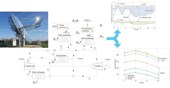
In this section, we first described the plant configuration and the optical and thermodynamic models employed to simulate the overall plant. The different performance indicators employed for comparing different locations and plant configurations are explained below. A pictorial representation of the plant, including the components of the thermodynamic subsystem, is represented in Figure 1.

2.1. Overall Plant Model

The designed hybrid CSP plant includes a parabolic dish that collects the sun radiation and heats a working fluid (dry air) flowing in the hybrid receiver situated at the focal point. According to the amount of solar irradiation quantified by the direct normal irradiance, G, and to the ambient temperature $T_L$, the integrated combustion chamber could release an energy flow in order to increase the fluid temperature up to a pre-fixed turbine inlet temperature, $T_3$. Therefore, the plant power output is approximately constant along the day; it oscillates only as a consequence of the variations of $T_L$. The HSRC includes a volumetric solar receiver, a combustion chamber, and a micro-Gas Turbine (mGT) operating on a recuperative Brayton cycle. The overall plant model includes mathematical submodels for all subsystems.

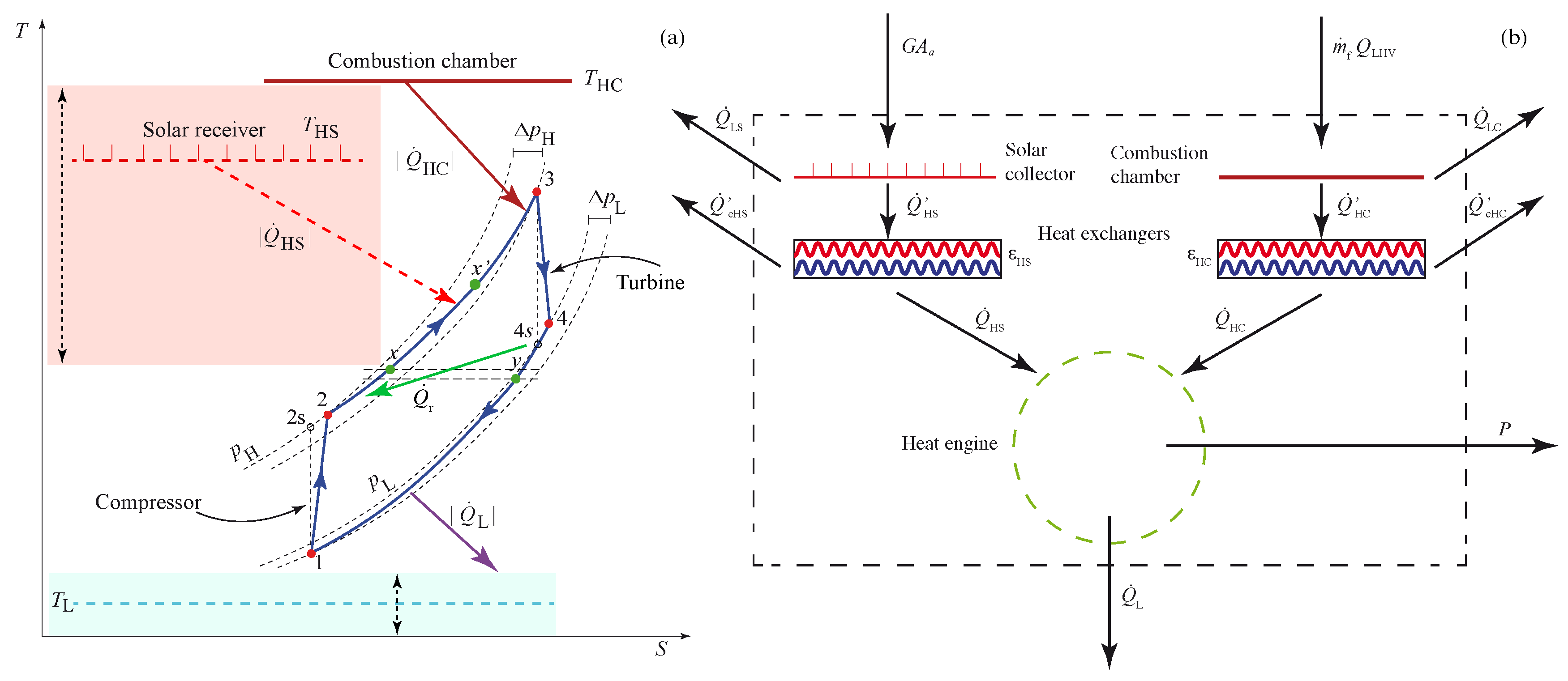
A thermodynamic representation of the overall system components is depicted in Figure 2. All heat transfers and losses included in the model are schematically represented. Details on all definitions, calculations, and equations can be found in previous works [21,22]. The overall plant thermal efficiency, $\eta$, is defined as the ratio between the net power output and the total energy input per unit time:

$$\eta =\frac{P}{G{A}_a+{\dot{m}}_f{Q}_{\mathrm{LHV}}}$$

(1)

where $A_a$ is the aperture area, ${\dot{m}}_f$ the fuel mass flow entering in the combustion chamber at any time, and $Q_{\mathrm{LHV}}$ the lower heating value of the fuel. The overall efficiency can be expressed as a combination of the efficiencies of the subsystems (${\eta }_s$, solar collector and receiver; ${\eta }_c$, combustion chamber; and ${\eta }_h$, heat engine efficiencies), the solar share, f (the fraction of the total heat input due to sun irradiance), and the effectiveness of the heat exchanges from the receiver and the combustion chamber to the fluid (${\epsilon }_{HS}$ and ${\epsilon }_{HC}$, respectively):

$${\displaystyle \eta ={\eta }_s{\eta }_c{\eta }_h\left[\frac{{\epsilon }_{HS}{\epsilon }_{HC}}{{\eta }_{c}f{\epsilon }_{HC}+{\eta }_s(1-f){\epsilon }_{HS}}\right].}$$

(2)

Explicit calculations to obtain this equation can be found in [21,22]. In the case of a purely solar operation, $f=1$ and $\eta ={\eta }_s{\eta }_h{\epsilon }_{HS}$, and for pure combustion, $f=0$ and $\eta ={\eta }_c{\eta }_h{\epsilon }_{HC}$.

2.2. Optical Model

The solar collector consists of a paraboloid shape dish with aperture diameter $D_{\mathrm{col}}$ and focal distance $f_{\mathrm{col}}$ that focuses the solar irradiation to a flat receiver. The receiver diameter $D_{\mathrm{rcv}}$ is determined as function of the concentration factor C, which is defined as $C=A_a/A_r$. $A_a$ stands for the irradiated aperture area of the collector and $A_r$ for the receiver area. The closed Brayton cycle employed in the plant requires a high upper temperature and a pressurized volumetric receiver. Thus, it becomes necessary to furnish the receiver with a transparent window with minimized reflection, radiation, and convection losses [24].

The energy delivered from the receiver to the working fluid depends not only on the optical losses, but also on the undesired heat transfer from the receiver to the surroundings. The latter are calculated as in [22,25], including convective, conductive, and radiation losses. Thus, the whole efficiency of the solar subsystem, ${\eta }_s$, is:

$${\eta }_s={\eta }_0-\frac{1}{GC}[\alpha \sigma (T_{HS}^4-T_L^4)+{\overline{U}}_L(T_{HS}-T_L)],$$

(3)

where ${\eta }_0$ stands for the optical efficiency, $\alpha$ refers to the emissivity of the receiver surface, $\sigma$ is the Stefan–Boltzmann constant, ${\overline{U}}_L$ is the overall conduction and convection heat transfer coefficient, and $T_{HS}$ is the solar collector temperature (see [21,22] for explicit definitions).

2.3. Power Unit Model

The gas turbine is considered to develop an irreversible recuperative Brayton-like cycle. The associated T-S diagram and main loss locations are depicted in Figure 2. The thermodynamic model was previously detailed and validated by our research group for central tower plants [22,26]. The model intends to be comprehensive and analytical to facilitate sensitivity and optimization analyses. Furthermore, it was developed to be applied to different working fluids (He, carbon dioxide, etc.) [22], and so, it relies on the assumption of a closed cycle. The validation shows that the results compare favorably with those of standard open cycle gas turbines [27].

Thus, the thermal efficiency of the micro-gas turbine, ${\eta }_h$, is calculated on the basis of a closed irreversible Brayton cycle considering a non-isentropic compressor and turbine, pressure losses in the heat absorption and heat release processes, and a non-ideal recuperator. The working fluid is dry air, considered as an ideal gas with temperature-dependent specific heats. Following the T-S diagram in Figure 2a, the gas is compressed from State 1 to State 2. Then, a first temperature rise up to $T_x$ is due to the recuperator connected to the turbine exit. Subsequently, during sunlight hours, the receiver releases heat to increase the temperature up to $T_{x^{\prime }}$. If this temperature is below the fixed turbine inlet temperature, $T_3$, a combustion chamber contributes with the corresponding heat. After State 3, the fluid is expanded in the turbine. Finally, the cycle is closed by means of a heat transfer to the recuperator and to the ambient surrounding through a heat exchanger. All those temperatures can be analytically expressed in terms of the compressor pressure ratio and parameters quantifying the considered irreversibilities. Explicit equations can be found in [22,26].

The micro-gas turbine efficiency is defined as ${\eta }_h=P/\left|{\dot{Q}}_H\right|$, where $|{\dot{Q}}_H|$ is the total heat input rate.

$$|{\dot{Q}}_H|=|{\dot{Q}}_{HS}|+|{\dot{Q}}_{HC}|$$

(4)

where $|{\dot{Q}}_{HS}|$ represents the heat rate input from the solar collector and $|{\dot{Q}}_{HC}|$ from the combustion chamber. The ratio between the solar heat input and the total one is the solar share, $f=|{\dot{Q}}_{HS}|/|{\dot{Q}}_H|$.

$$|{\dot{Q}}_{HS}|=\dot{m}{\int }_{T_x}^{T_{x^{\prime }}}{c}_w\left(T\right)dT=f\left|{\dot{Q}}_H\right|$$

(5)

$$|{\dot{Q}}_{HC}|=\dot{m}{\int }_{T_{x^{\prime }}}^{T_3}{c}_w\left(T\right)dT=(1-f)\left|{\dot{Q}}_H\right|$$

(6)

The heat release to the ambient surrounding is expressed as:

$$|{\dot{Q}}_L|=\dot{m}{\int }_{T_1}^{T_y}{c}_w\left(T\right)dT$$

(7)

In these equations, $c_w\left(T\right)$ represents the temperature-dependent constant pressure specific heat of the working fluid. Thus, the power output released by the heat engine $P=|{\dot{Q}}_H|-|{\dot{Q}}_L|$.

2.4. Hybridization Model

It is assumed that the operation objective of the solar dish is to provide a constant power output, independently of the solar and meteorological conditions, all year around. Thus, a combustion chamber is incorporated in such a way that it releases a variable heat rate that complements solar input to guarantee a constant turbine inlet temperature. This means that the theoretical capacity factor of the plant is 100%.

The efficiency of the combustion chamber, ${\eta }_c$, once having elected the fuel to be burned and the fuel-air equivalence ratio, can be considered as a constant parameter. In real equipment, it could slightly change with the fluctuations of the fuel-air equivalence ratio, the composition of the fuel, its temperature, and several other variables. The heat received by the working fluid from the combustion chamber, ${\dot{Q}}_{HC}$, can be written as:

$$|{\dot{Q}}_{HC}|={\epsilon }_{HC}|{\dot{Q^{\prime }}}_{HC}|={\epsilon }_{HC}{\eta }_c{\dot{m}}_f{Q}_{\mathrm{LHV}}$$

(8)

By expressing the effectiveness of the heat exchanger in between the combustion chamber and the thermal cycle as ${\epsilon }_{HC}=(T_3-T_{x^{\prime }})/(T_{HC}-T_{x^{\prime }})$ (see Figure 1), the heat released, in terms of temperatures, is:

$$|{\dot{Q}}_{HC}|=\dot{m}{c}_w\left(T_3-T_{x^{\prime }}\right)=\dot{m}{c}_w{\epsilon }_{HC}\left(T_{HC}-T_{x^{\prime }}\right)$$

(9)

The effective temperature in the combustion chamber is denoted as $T_{HC}$. As fluctuations in G and $T_L$ will be taken into account, the fuel mass flow to be burned in the combustion chamber will also be a time-dependent function, in general given by:

$${\dot{m}}_f=\frac{\dot{m}{c}_w(T_3-T_{x^{\prime }})}{{\eta }_c{Q}_{\mathrm{LHV}}{\epsilon }_{HC}}$$

(10)

where $T_{x^{\prime }}$ will vary with the solar irradiance and ambient conditions.

The final electrical energy produced, $E_{\mathrm{elec}}$, allows quantifying the actual electricity output. It can be calculated from the net mechanical power output, P, the efficiencies of the generator and alternator systems (${\eta }_{\mathrm{gen}}$ and ${\eta }_{\mathrm{alt}}$), and the mechanical efficiency, which represents the ratio between the shaft power and the gas turbine rotor power, ${\eta }_{\mathrm{mec}}$. Thus, the net electrical energy output can be written as:

$$E_{\mathrm{elec}}={\eta }_{\mathrm{gen}}·{\eta }_{\mathrm{alt}}·{\eta }_{\mathrm{mec}}·P.$$

(11)

2.5. Economic Performance Indicators

Currently, it is necessary to evaluate not only the thermodynamic and technical aspects of a power plant, but also to assign costs and to identify the intensity of harmful emissions. Therefore, once the thermodynamic performance of the plant is established, the second stage is to assign costs: investment and initial installation costs, $C{I}_0$, costs incurred during operation (indirect and maintenance costs $C_{\mathrm{O}\&\mathrm{M}}$, such as labor to operate the plant or water for cleaning the mirrors), and fuel costs in the case of hybrid plants, $C_{\mathrm{fuel}}$. The levelized cost of electricity is an economic indicator commonly employed to compare power plants of different sizes, and it serves to determine the minimum electricity sale price needed to recover investment and operation costs over the expected lifetime of the plant [28]. Equation (12) describes the LCoE calculation following the International Energy Agency (IEA) definition [29,30]. It is the ratio between the sum of the total costs and the sum of the electrical energy production, $EE$, over the expected lifetime, which is usually assumed to be $n=25$ years for solar plants. Both sums are discounted at a constant rate r over the lifetime of the plant.

$$\mathrm{LCoE}=\frac{{\displaystyle \sum _{i=1}^n\left(C{I}_0+C_{{\mathrm{O}\&\mathrm{M}}_i}+C_{{\mathrm{fuel}}_i}\right){(1+r)}^{-i}}}{{\displaystyle \sum _{i=1}^{n}E{E}_i{(1+r)}^{-i}}}.$$

(12)

Neither the decommissioning costs, nor the interest accrued during the construction are considered, as the construction time for these parabolic dishes is considered lower than one year.

• In this paper, the total investment costs, $C{I}_0$, are derived from the sum of the equipment cost, $C_{\mathrm{eqp}}$, the cost of equipment installation, $C_{\mathrm{inst}}$, civil engineering costs, $C_{\mathrm{civil}}$, and contingencies, $C_{\mathrm{cont}}$. $C_{\mathrm{civil}}$ summarizes the costs from the system engineering, tracking, basement, cabling, and assembly. $C_{\mathrm{cont}}$ is a purely financial cost associated with the risk and uncertainty of the project, based on previous experience regarding similar technologies.

  $$C{I}_0=\sum C_{\mathrm{eqp}}+C_{\mathrm{inst}}+C_{\mathrm{civil}}+C_{\mathrm{cont}}.$$

  (13)
  In turn, the equipment is considered as formed by the HSRC ($C_{\mathrm{HSRC}}$), comprised of the micro-gas turbine, the compressor, the solar receiver (control system, absorber, and pressure resistant glass window), and combustion chamber, as well as other auxiliary items such as the insulation and housing. Furthermore, the equipment includes the dish itself ($C_{\mathrm{dish}}$), which incorporates the parabolic mirror, facets, tracking system, and installation pedestal. Finally, the generator costs ($C_{\mathrm{gen}}$) arise from the electrical generator costs (with the power electronics and control system).

  $$C_{\mathrm{eqp}}=C_{\mathrm{HSRC}}+C_{\mathrm{dish}}+C_{\mathrm{gen}}.$$

  (14)
• The term $C_{{\mathrm{O}\&\mathrm{M}}_i}$ in Equation (12) represents the annual cost from operation and maintenance in year i. It is comprised of cleaning word, water, and an annual share of equipment costs, $C_{\mathrm{eqp}}$.
• $C_{{\mathrm{fuel}}_i}$ is a strongly uncertain component of costs. It is the annual fuel cost in year i associated with hybridization. Not only fuel price variations can be found of course among different countries, but also, it is likely to suffer fluctuations during the year, even in the same region.
• $E{E}_i$ is the electrical energy produced in year i. It is directly associated with the plant thermal efficiency. An optimized design from the optical and thermodynamic viewpoints makes the denominator of the LCoE increase and, so, reducing the LCoE values.
• Finally, r is the discount rate, considered as the sum of the inflation rate and the interest. A standard fixed value is usually taken for numerical estimations.

3. Numerical Data for Computations And Validation

In order to perform numerical computations and analysis, dish sizes and power output levels were taken from Semprini et al. [31]. In particular, two power levels were chosen, 7 and 30 kWe. Aperture and receiver areas, and so, concentration factors, were taken from that paper, as well as the optical efficiency of the dishes. Independent simulations of optical efficiency were made in our group by using the software Tonatiuth [32]. Discrepancies from the values obtained by Semprini et al. [31] were very small (below 0.5%), so those values were assumed for calculations. All the optical parameters, as well as those from the combustion system and for the Brayton cycle developed by the micro-gas turbine, are collected in

Table 1. Parameters extracted from Semprini et al. [31] (*) and those taken to validate our model. The validation target is the micro-gas turbine Capstone C30 [33].

	Subsystem			Study Cases
				$\mathit{P}=30$ kWe	$\mathit{P}=7$ kWe
	Collector area *		$A_a$ (m${}^2$)	$211.8$	$52.80$
	Diameter receiver *		$A_r$ (m)	$0.3879$	$0.1941$
	Concentration factor *		C	1792	1784
Solar	Optical efficiency *		${\eta }_0$	$0.9083$	$0.9086$
system	Heat exchanger efficiency		${\epsilon }_{HS}$	$0.7951$	$0.7923$
	Emissivity coefficient		$\alpha$	$0.1$	$0.1$
	Convection and conduction
	effective coefficient		${\overline{U}}_L$ (W/(m${}^2$K))	5	5
Combustion	Combustion chamber efficiency		${\eta }_c$	$0.97$	$0.97$
system	Heat exchanger efficiency		${\epsilon }_{HC}$	$0.97$	$0.97$
	Turbine efficiency *		${\epsilon }_t$	$0.76$	$0.74$
	Compressor efficiency *		${\epsilon }_c$	$0.77$	$0.76$
Brayton cycle	Turbine inlet temperature *		$T_3$ (K)	1173.15	1173.15
micro-gas	Pressure ratio *		$r_p$	3.84	3.65
turbine	Air mass flow *		$\dot{m}$ (g/s)	$337.9$	$88.1$
	Recuperator effectiveness		${\epsilon }_r$	$0.85$	$0.85$
	Pressure drop	(Process 2 → 3)	$\Delta p_H/p_H$ (%)	$12.5$	$12.5$

.

On-design direct normal irradiance was taken as $G=780$ W/m${}^2$ and ambient temperature as $T_L=298.15$ K. The data used to simulate the micro-gas turbine were adapted to reproduce the turbine Capstone C30 [33], the same analyzed by Semprini et al. [31]. Generator and alternator efficiencies (${\eta }_{\mathrm{gen}}$ and ${\eta }_{\mathrm{alt}}$) were set at 96% and the mechanical efficiency, ${\eta }_{\mathrm{mec}}$, at 98% [34]. For the case of 30 kWe, the deviation of our calculations for the thermal efficiency and the power output was below 3.5% and 0.4%, respectively. For the lowest power output, 7 kWe, differences were below 4.7% for thermal efficiency and 2.2% for power output. These results for the validation were obtained by taking polynomial fits for the specific heat of air from RefProp 9.1 [35]. The same model for the gas turbine was validated for other thermosolar systems (central towers) at higher power levels (megawatt scale) in previous works [22,26,27].

Assembling a wide variety of information sources including literature and direct personal communications, specific cost functions were determined to calculate the final purchasing costs of each element, based on the size and operating conditions. This hybrid solar power plant with a specific HSRC is still not currently marketed; however, to draw price comparisons, a prototype of an integrated combustion chamber and mGT based on Ragnolo et al. [36,37] was employed. Many factors will affect the final purchasing costs such as the number of units ordered or the state of the market. Therefore, the data provided here are useful for comparison between locations and operation modes, but they cannot be deemed as an exact cost prediction of a hybrid solar gas turbine dish. The purchased equipment costs were estimated assuming a production rate of 1000 modules year, as described in [38].

Following recommendations from Peters and Timmerhaus [39], the cost of equipment installation $C_{\mathrm{inst}}$ was equal to 20% of the initial equipment purchasing costs. Likewise, civil cost $C_{\mathrm{civil}}$, including project engineering costs, was calculated as 8 to 23% of the total $C_{\mathrm{eqp}}$ (the most pessimistic was taken [30]). For the unforeseen technical problems during the construction or operations, the IEA estimates a total contingency cost, $C_{\mathrm{cont}}$, equal to 10% of the total initial investment cost. Contrary to initial investment costs, operation and maintenance costs $C_{\mathrm{O}\&\mathrm{M}}$ are incurred during the power plant lifetime, such as water consumption for occasional mirror facet cleaning (50 L/m${}^2$ per year) and costs related to reparation or replacement of damaged components, calculated as a percentage of the initial equipment cost (i.e., 2%/y for the mGT and receiver, 3%/y for the elements of the parabolic dish, and 4%/y for the control system). Due to the small plant size, no specific operation labor costs were considered, and the technician or operator was included within the maintenance costs detailed above.

Fuel costs strongly depend on system location. The policies of each country establish taxes that greatly rely on financial or economic cycles and particular conditions. IEA defines international prices for the fuel industry in order to perform global statistics. For Spain, fuel cost data were taken from 2018 and were set to 26.41 €/MWh thermal [40] for natural gas. This price was chosen in a quite pessimistic scenario, including taxes, transport, and commercialization expenses. The lower heating value for natural gas considered was $47.146\times {10}^6$ J/kg [41]. The discount rate, r, was assumed to be 9% [42]. All the data considered for LCoE calculations are compiled in

Table 2. Cost parameters used to estimate the Levelized Cost of Electricity (LCoE) and the corresponding sources. Total costs appearing in Equation (12) are obtained as the simple product of specific costs by the plant nominal power output, except for fuel costs that are already expressed in €/MWh.

Cost Type		Specific Cost (€/kWe)	Source
	$C_{\mathrm{HSRC}}$	480	[42]
$C_{\mathrm{eqp}}$	$C_{\mathrm{dish}}$	1550	[42]
	$C_{\mathrm{gen}}$	226.8	[43]
$C_{\mathrm{inst}}$		20 % $C_{\mathrm{eqp}}$	[39]
$C_{\mathrm{civil}}$		23 % $C_{\mathrm{eqp}}$	[30]
$C_{\mathrm{cont}}$		10 % ($C_{\mathrm{eqp}}$+ $C_{\mathrm{inst}}$+ $C_{\mathrm{civil}}$)	[30]
$C_{\mathrm{O}\&\mathrm{M}}$		2 % $C_{\mathrm{HSRC}}$+ 3 % $C_{\mathrm{dish}}$+ 4 % $C_{\mathrm{gen}}$	[6,28]
$C_{\mathrm{fuel}}$		26.41 / MWh	[40]

.

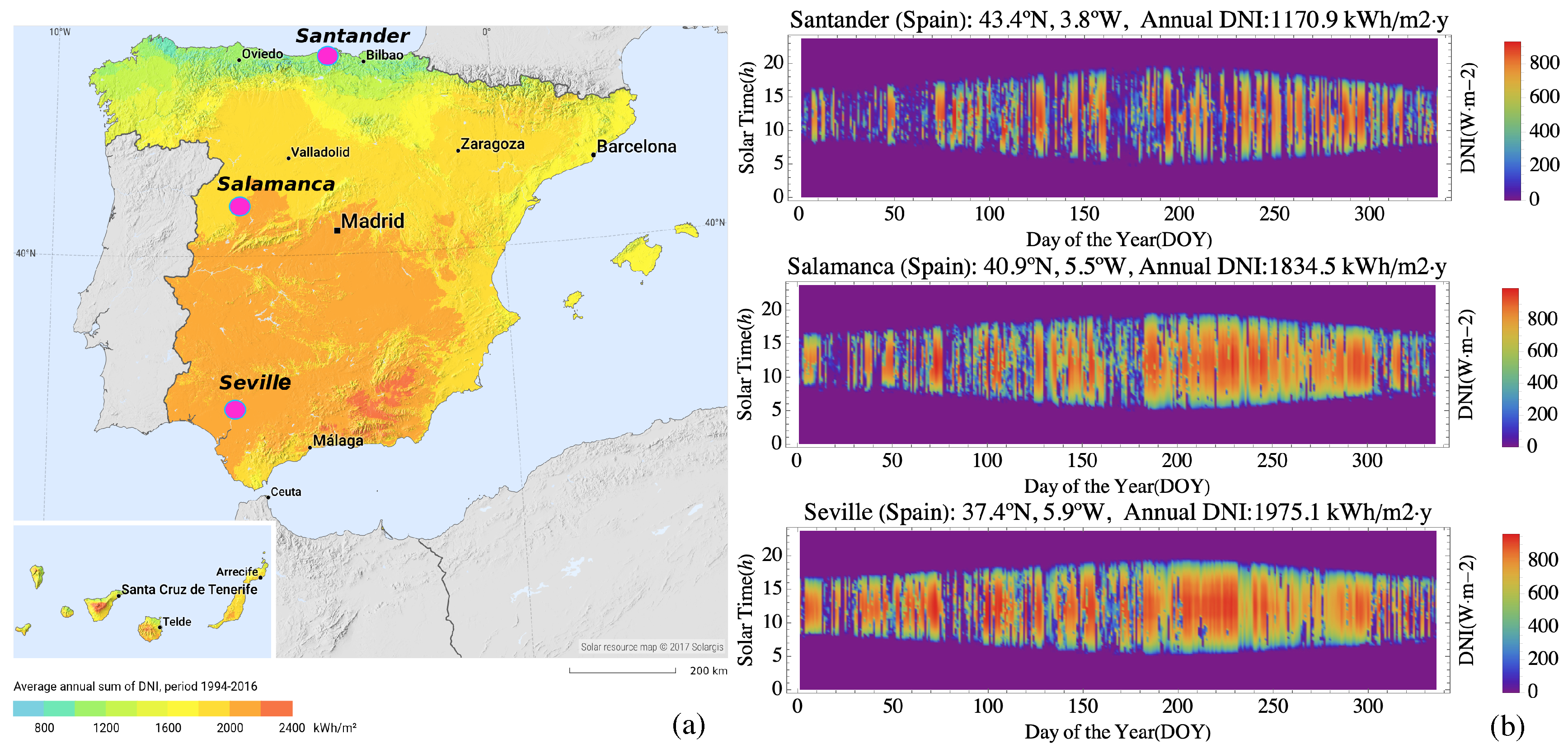
After validation, seasonal and annual analysis was done for the mentioned power outputs, for recuperative and non-recuperative micro-gas turbines, and for three locations in Spain with quite different latitudes and meteorological conditions. The locations of the three cities considered in Spain are shown in Figure 3a.

• Santander is located in the north of Spain, with latitude 43.4° N, on the Atlantic coast, at sea level. In principle, solar conditions are not favorable; the climate is oceanic and humid, with plenty of cloudy days (see Figure 3b) and mild temperatures (the mean annual temperature is 14.1 °C). The average annual Direct Normal Irradiation (DNI) is about 1170 kWh/m${}^2$. This location was elected to numerically evaluate the differences from the other two, a priori, more interesting locations.
• On the other side, Seville is located in Andalusia, in the south of Spain (latitude 37.4° N). The average annual DNI is almost twice that of Santander, about 1975 kWh/m${}^2$. Several CSP commercial and prototype installations have been developed in the last few years around Seville. The weather is dry and warm, and sunny days are usual in any season. It has a typical Mediterranean climate: dry and hot summers and mild temperatures in winter, when rain is concentrated. Temperatures during daytime in summer can reach values above 30 °C (see a sample day in Figure 4) and are rarely below 5 °C in winter. The yearly average temperature is 18.6 °C. The peak DNI can be quite above 800 W/m${}^2$ in any season (see also the days taken for Figure 4). The altitude above sea level is low, about 7 m. On average, there are about 50 rainy days per year (above 1 mm of rainfall).
• Salamanca is located in between Santander and Seville, on a plateau at about 800 m above sea level. It has a dry continental climate. Summers are dry and hot and winters cold with not much rain. The DNI is only slightly below that of Seville, about 1834 kWh/m${}^2$. Annual precipitation is about 373 mm, and there are only 64 days per year with more than 1 mm of rainfall. During winter months, the daily average temperatures could be around 5 °C (from December to March). The annual mean temperature in Salamanca is 12.1 °C.

Ambient temperatures were taken from the Spanish Meteorological National Agency (AEMET) [46]. Temperatures were averaged each 30 min. Nevertheless, the absence of several DNI data for some locations from AEMET made it necessary to take data from the Copernicus Atmosphere Monitoring Service (CAMS) [45], also each 30 min. With this time lapse, the working temperature of the solar receiver ($T_{HS}$ in Figure 2a) was dynamically obtained by balancing the solar energy input in the receiver and the heat extracted by the working fluid. The sample curves of the DNI and ambient temperature in Figure 4 for particular days of winter and summer in the three locations were not smoothed nor averaged to visualize the differences on the same particular days among the three locations. It is particularly interesting, for instance, that in summer, it is possible, as shown in Figure 4b,d, that Seville and Salamanca reach the same peak DNI values. The temperature curves are roughly parallel, but displaced. The $T_L$ values for Salamanca are always between 5 and 10 °C below.

All the greenhouse emissions that will be shown below were calculated from standard emission factors for greenhouse gases [47].

4. Daily and Seasonal Behavior of Plant Records

The evolution of the main plant output records such as efficiencies, power output, solar share (the fraction of heat input to the working fluid from the Sun with respect to the total), and main temperatures were estimated from the model for the three locations and particular days representative of each season.

Figure 5 shows the evolution of the main efficiencies and solar share for two particular days, in winter and summer. These days are 13 December 2017 and 13 June 2018. The shape of the DNI and ambient temperature for these days is shown in Figure 4. Some of the curves correspond to cloudy days, but were not smoothed nor averaged, in order to analyze the behavior of the dish in conditions as close to reality as possible. Annual averages will be shown in the next section. The curves correspond to the power output level of 30 kWe and include recuperation. Solar subsystem efficiency, ${\eta }_s$, is really high and almost constant during daytime, always around $0.9$. Heat engine efficiency, ${\eta }_h$, is stable because the turbine inlet temperature is a fixed input parameter. Overall efficiency, $\eta$, is regular at night and slightly below ${\eta }_h$ (the difference is associated with combustion efficiency) and decreases when the solar dish is operating because its losses are added to those of the heat engine. Solar share is also depicted in Figure 5. It has a behavior in concordance with the DNI’s evolution (see Figure 4). In some situations, it reaches its maximum attainable value (in the cases considered for a DNI approximately over 750 W/m${}^2$), so for the considered dish dimensions, a defocusing system should be designed to avoid overheating and damage.

The insets in Figure 5 show for two different cases the amplitude of the fluctuations of overall efficiency and power output. The latter are essentially associated with ambient temperature evolution and very small in relative terms. Nevertheless, the fluctuations of overall efficiency are appreciable, in the pictures shown reaching 15% in Santander during the considered winter day and almost 30% for Seville in summer (see Figure 5, bottom right). These fluctuations arise, apart from meteorological oscillations, from the solar subsystem operating or not, i.e., when the plant works with solar heat input, solar collector and receiver losses decrease the overall efficiency up to 30% in the cases shown. It is important here to recall that the factor ${ϵ}_{HS}\simeq 0.79$ (see Table 1) is considered as the effectiveness of the solar receiver acting as a heat exchanger.

The hourly evolution of air temperatures in the main thermodynamic cycle states is depicted in Figure 6. The notation for those states is shown in Figure 1 and Figure 2a. As mentioned before, the turbine inlet temperature, $T_3$, is considered as a fixed input parameter (about 1173 K). Thus, the gas temperature before entering into the recuperator, $T_x$, is also fixed (about 850 K), although it depends on the ambient temperature. $T_{x^{\prime }}$ is the temperature after the solar receiver, which depends on the DNI. When the solar share is above $f=1$, $T_{x^{\prime }}=T_3$. The solar receiver operating temperature, $T_{HS}$, also fluctuates with the DNI and ambient temperature and needs to be controlled to avoid engine damage in periods with good solar conditions. Therefore, in very good conditions, the solar receiver increases the gas temperature about 300 K.

The simulations of plant records were also performed without recuperation in order to analyze efficiencies and temperatures. A particular case is shown in Figure 7. It corresponds to Salamanca during a summer day. The curves should be compared with those in the right middle panels in Figure 5 and Figure 6. On the one hand, engine efficiency, ${\eta }_h$, and overall efficiency, $\eta$, decrease to about half of the recuperative configuration. The maximum solar share decrease is similar. On the other hand, the temperature of the fluid after the solar receiver, $T_{x^{\prime }}$, does not reach the fixed turbine inlet temperature, so the dish is always operating within a partial combustion mode. In this case, defocusing would not be necessary. The difference between instantaneous fuel consumption with or without recuperation for the same conditions is shown in Figure 8 (Salamanca, summer, and $P=30$ kWe).

5. Monthly and Annual Plant Estimations

In this section, we intended to provide a monthly evolution of dish output records and also the annually averaged ones, comparing among the three elected locations and power outputs. The effects of recuperation from this perspective also deserve an analysis.

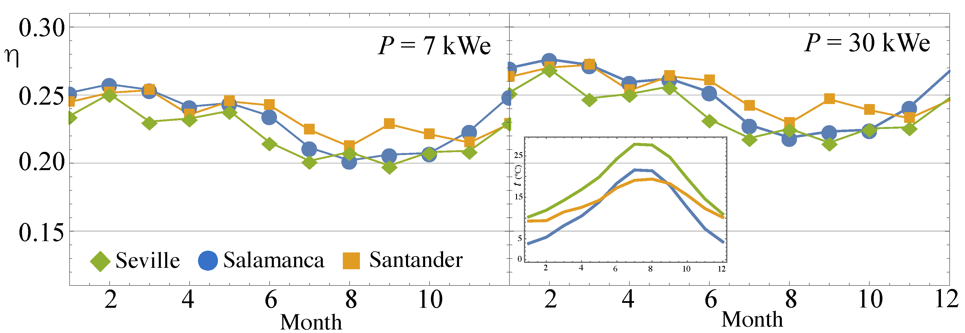
As can be observed in Figure 9 for the lowest level of power output, $\eta$ oscillates between 0.20 and 0.25 for a recuperated plant. During summer months, from approximately June to October, it shows a dip for any location because of the average increase of the ambient temperature. For $P=30$ kWe, the monthly evolution is similar, but the numerical values of the overall efficiency are larger for all places. It is important to have in mind here (looking at Table 1) what the main differences between both power levels with respect to the model input parameters are. Although the size of the dish in both cases is different, the concentration factor, optical efficiency, and other parameters from the solar subsystem are similar. The combustion system and losses parameters in the Brayton cycle are also analogous; the pressure ratios are slightly different; and the air mass flows are quite different. The combination of these factors leads to the minimum efficiency in Seville (for $P=30$ kWe) during September. It is about 0.21. The maximum is achieved in the coldest location, Salamanca, in February, approximately 0.28. This suggests that at this modeling level, the most important factor for the monthly evolution of overall efficiency is the average ambient temperature. This fact can be corroborated by looking at the temperature profile shown in the inset of Figure 9. Almost without exception, for any month, the lowest average ambient temperature corresponds to the highest overall thermal efficiency.

Table 3. Comparison of the annual results for different locations for hybrid and pure combustion modes.

Location	Seville		Salamanca		Santander
Power Output	7 kWe	30 kWe	7 kWe	30 kWe	7 kWe	30 kWe
Hybrid Operation Mode
Overall efficiency (%)	22.14	23.88	23.18	24.95	23.35	25.16
Averaged solar share, f (%)	41.12	41.35	30.42	30.59	20.99	21.18
Energy generated (MWh${}_e$)	58.49	251.06	60.14	257.54	59.22	253.89
Fuel consumption (t)	14.00	55.63	15.67	62.29	17.39	69.12
Combustion Operation Mode
Energy generated (MWh${}_e$)	60.52	259.141	62.26	265.96	60.32	258.29
Fuel consumption (t)	20.56	81.83	20.63	82.11	20.56	81.83
Mode Comparison
Fuel savings (t)	6.56	26.20	4.96	19.82	3.17	12.71
Fuel savings (%)	31.91	32.02	24.04	24.14	15.42	15.53
Net reduction of CO${}_2$ (t)	16.23	64.83	12.28	49.04	7.84	31.45
Net reduction of CH${}_4$ (kg)	306.99	1226.69	232.26	927.77	148.25	595.09
Net reduction of N${}_2$O (kg)	29.81	119.09	22.55	90.08	14.39	57.78

contains the yearly average global efficiencies. For all locations, the average $\eta$ is slightly larger for the highest power output. The differences among locations are also small. Santander has the best records. This is associated with a lower solar share: a larger solar share means that the solar subsystem (and its losses) is coupled for more time to the power unit, decreasing the overall efficiency. Yearly solar shares are the largest for Seville, about 41%, and the smallest for Santander, about 21%.

The energy produced by month is outlined in Figure 10. It is approximately constant for both power levels, although oscillations are smaller for 7 kWe. The stability of the produced energy means that the objective of the plant is fulfilled: to guarantee steady output records by means of hybridization. Table 3 contains annual averages of the energy generated, both in hybrid operation mode and for pure combustion. For the same level of power output, the energy produced is similar in all locations.

The evolution during the year of fuel consumption on the basis of natural gas is depicted in Figure 11, where the shaded areas represent the fuel savings along the year. Numerical values are also included in Table 3, as well as yearly emissions in real units. The decrease of fuel consumption is perfectly clear around summer months. More evident in Seville, but even in Salamanca, the savings are also noteworthy in other seasons. The fuel savings are largest in Seville and amount to about 31%. The lowest correspond to Santander, because of its worse irradiance data. There, fuel consumption is almost double compared with Seville. Salamanca, at an intermediate latitude, but also with lower mean temperatures, leads to savings of about 24%. This is smaller than Seville, but they are remarkable numbers anyway. All the data in Figure 11 and Table 3 refer to a plant layout that incorporates a recuperator. Of course, it increases thermodynamic efficiency and decreases fuel consumption, but conversely greatly increase operating temperatures (as explained before by Figure 5, Figure 6 and Figure 7).

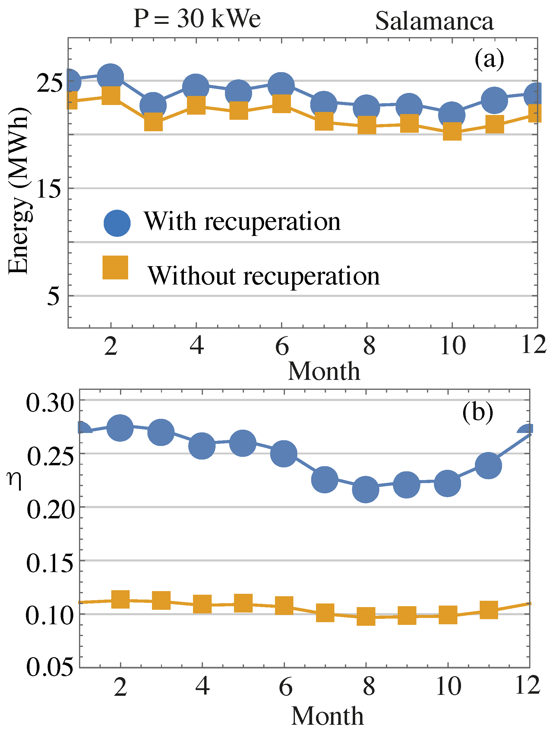
Monthly produced energy, overall efficiency, and solar share for $P=30$ kWe and Salamanca as an example are depicted in Figure 12 for two plant layouts: with and without recuperation. The energy produced (see Figure 12a) is similar in both configurations because the same turbine inlet temperature is fixed in both cases. The differences between lines representing overall efficiency are substantial (see Figure 12b). The efficiency for the recuperated plant is, in all months, above twice the non-recuperated one. Although, fixing the same scale for both, a seasonal decrease during summer is less evident for the non-recuperated plant. This is explained in Figure 12c, which contains a plot of solar share. During summer, solar share is quite larger for the recuperated plant: the solar subsystem contributes to a larger extent, so the losses it incorporates in the whole system decrease the thermal efficiency.

Fuel consumption and savings are also plotted in Figure 13, at the same scale to visualize the differences between those two modes. Lines are parallel, but displaced (approximately, monthly consumption is 2.5 times larger without recuperation), so the savings are similar by a yearly average.

6. Levelized Cost of Electricity

As explained in Section 2, the levelized cost of electricity is the economic indicator selected to analyze the performance of the hybrid solar dish from the perspective of the price of the electricity produced. It is always difficult to assign costs to the components and operation of a system that is still under development, and the obtained net values can have an appreciable uncertainty. Nevertheless, the comparison between different locations, different weather conditions, different plant layouts, etc., within the same scheme can reveal interesting aspects. All the estimations were performed with the data considered in Section 3. The three locations chosen were analyzed for the turbine working in a standard combustion-only model (assuming natural gas fueling and recuperation) and in a hybrid solar mode on an annual basis. To survey the values of the LCoE with the aim the interval of power output levels, four values of power output, between 7 and 30 kWe, were analyzed.

Figure 14 collects the evolution of the LCoE with the power output, and

Table 4. Summary of the LCoE and specific emissions for different power outputs and locations.

Power Output		7 kWe	15 kWe	23 kWe	30 kWe
LCoE (€/MWh${}_e$)
Seville		130.12	133.24	129.33	123.90
Salamanca		136.14	139.42	135.44	129.71
Santander		148.28	151.70	147.32	140.86
Hybrid Mode Specific Emissions (kg/MWh${}_e$)
	CO${}_2$	592	600	584	548
Seville	CH${}_4$	11.21	11.35	11.06	10.37
	N${}_2$O	1.09	1.10	1.07	1.01
	CO${}_2$	645	654	637	598
Salamanca	CH${}_4$	12.20	12.37	12.06	11.32
	N${}_2$O	1.18	1.20	1.17	1.10
	CO${}_2$	727	737	718	674
Santander	CH${}_4$	13.75	13.94	13.58	12.74
	N${}_2$O	1.45	1.35	1.32	1.24

contains the particular numerical results. Figure 14 shows a non-linear evolution of the LCoE with the power output level. It increases from 7 kWe up to 15 kWe, where it presents a maximum, and then, it decreases to a minimum value at the highest power output analyzed, 30 kWe. The values of the LCoE for combustion-only are always above the hybrid mode, and the differences are substantial. In combustion-only mode, the LCoE is smallest for Salamanca, probably due to its lower mean ambient temperatures, the only parameter influencing the thermodynamics of the system associated with the site location in this mode. Roughly, Salamanca’s mean annual temperature is 12.1 °C; Seville’s is 18.6 °C; and Santander’s is in between, 14.1 °C. The LCoE for combustion-only is in the interval $(152-168)$ €/MWhe.

In hybrid operation, the LCoE has a similar evolution with the power output, but the savings in operation costs because of the reduced fuel consumption displaces the curves to lower values. It is important to have in mind here that the same equipment costs were considered to perform these calculations, i.e., the costs of the HSRC and dish were considered the same in both modes. In hybrid mode, Santander reaches the highest values of the LCoE due to its worse DNI records, and Seville gives the lowest LCoE values. However, the values of the LCoE for Salamanca are close to those of Seville. Its lower DNI values are compensated by its also lower mean ambient temperatures. In numerical terms, the best record (see Table 4) is obtained in Seville for 30 kWe and is about 124 €/MWhe. In relative terms, this value is about 18% lower than the analog for pure combustion mode.

Of course, a key (and uncertain) factor in the particular values of estimated LCoE is the cost of fuel. For the calculations shown in Figure 14, C${}_{\mathrm{fuel}}=26.41$ €/MWh [40], which is a realistic (and pessimistic) price in Spain for 2018. To deepen the influence of fuel costs, Figure 15 shows the slope of the dependence of the LCoE with fuel costs in a wide interval of prices. In hybrid operation, of course, the increase of the LCoE with the price of natural gas is largest in Santander and smallest in Seville.

The final purpose of this section is to present a brief comparison of the LCoE results obtained within our model with other estimations for the same type of system and for other renewable systems for electricity production. As mentioned by Giostri et al. [34], an LCoE equal to approximately 160 €/MWhe could guarantee competitiveness with reference CSP technologies, for instance parabolic trough or solar towers located in the Mojave desert, USA. In the study by Giostri et al., an evolution of the LCoE with receiver specific cost was presented. This was motivated by the prototypal stage of high temperature solar receiver technologies. For a specific cost for the receiver similar to that assumed by us in Table 2, Giostri et al. obtained an LCoE of about 180 €/MWhe for a 33 kWe solar dish located in Las Vegas, slightly above our results, but entirely comparable (see Figure 16 in [34]). In the last few years, a prototype parabolic dish with hybrid Brayton technology was developed with funding from the European Commission (2013–2017), the so-called OMSoP project [14]. The prototype dish, capable of supporting a micro-gas turbine up to 15 kWe, was built in Italy (Casaccia, Rome). Probably, the experimental period for data acquisition after complete installation was not sufficiently long to extract robust conclusions, but it was argued that LCoE values between 100 and 150 €/MWhe could be achieved in a location with mild solar conditions [48]. This interval is slightly below the one obtained in this work, but also comparable.

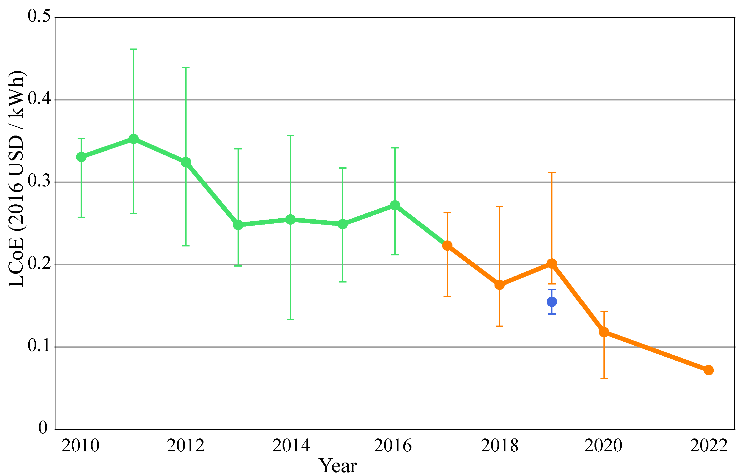
Figure 16 and Figure 17 allow comparing our results with those of the International Renewable Energy Agency published in 2018 [49]. The figures were obtained just by adding our estimations to the data in that report. In Figure 16, a timeline of the LCoE evolution from 2010–2022 is represented, attending to the geographical location of the CSP plants. In Figure 17, different renewable technologies are analyzed in the period 2016–2017. From both figures, the results obtained in this work are reasonable. In any case, it should not be forgotten that the LCoE strongly fluctuates depending on each country’s pricing policies, the state of the market, the estimated number of manufactured units, and fuel costs. The fact that an increasing number of research works, with different perspectives and approaches, lead to comparable economic indicators makes the confidence about realistic electricity sale prices from this technology more robust.

7. Summary and Conclusions

In this work, we presented a complete model to analyze the performance of a solar dish working on a hybrid Brayton thermodynamic cycle. The model is simple enough to incorporate in an attainable way all the main subsystems that form the global plant, including the most relevant sources of losses, optical, mechanical, and thermodynamic. The micro-gas turbine is considered as integrated with the receiver, i.e., it is taken as a hybrid solar receiver combustor. The model is capable of predicting, with good precision (as is shown in the validation process), the main output records of the plant, not only at on-design conditions, but also at any time for any particular location and meteorological condition. The thermodynamic parameters such as efficiencies and temperatures at any thermodynamic cycle step can be estimated dynamically. Furthermore, the key indicators to analyze the marketing possibilities of this technology such as the LCoE or specific emissions can be estimated.

The model was applied to analyze the possibilities of this solar dish in a power output level from 7 to 30 kWe in three locations in Spain with quite different latitudes (south, middle, and north), DNI levels, and mean temperatures. The daily fluctuations of all subsystems’ efficiency were analyzed for particular days in any season. It was shown how hybridization allows obtaining an almost constant power output, if that is the aim of the plant. Overall efficiencies of about 0.30 are achievable when the plant design includes a recuperator for all the surveyed locations and seasons. Non-recuperated plant layouts are also feasible, but two consequences are straightforward. First, the overall plant thermal efficiency greatly decreases (up to one half of the recuperated plant), and the operating temperature of the solar receiver also decreases. For a recuperated turbine, it can reach values above 1200 K if solar conditions are good, and for a non-recuperated receiver, the temperatures are about 200 K lower. This, of course, would affect the type of materials necessary to build the receiver and its costs. The influence of recuperation is also important from the viewpoint of solar share. When the micro-gas turbine incorporates a recuperator, it is actually possible that for DNI values over 800 W/m${}^2$, solar share reaches one, and so, some security system is necessary to avoid damages in the turbine. On the other side, when no recuperation is considered, solar share barely reaches 0.6. This means that the combustion of a fuel is imperative to reach the turbine inlet temperature (which was considered as a fixed design input, about 1173 K).

A monthly analysis allowed concluding that thermal efficiency oscillates along the year, reaching its highest values during the coldest months. Maximum values are slightly larger for the highest power output level, 30 kWe. The smallest are predicted during summer for the lowest power output. It was also shown that the monthly energy production is almost constant. Emissions and fuel savings were also analyzed, from monthly and yearly perspectives. By comparing a pure combustion operation mode with a solar hybrid one, it was demonstrated that fuel savings can amount to between 15% for a location with poor solar conditions and 32% in Seville, the south of Spain. Specific emissions of CO${}_2$ were estimated to be about 0.548 t/MWhe in the best case (Seville and 30 kWe). In a location at the center of Spain with relatively good solar conditions and lower annual mean temperature, Salamanca, specific emissions are also below 0.6 t/MWhe (see Table 4).

The levelized cost of electricity was also computed for several power outputs and the same locations. A previous survey was performed to select actual and realistic cost parameters. A non-linear behavior for the LCoE as a function of power output level was reported in the surveyed interval of power outputs. In the range between 7 and 30 kWe, the LCoE increases up to 15 kWe and then decreases. At 30 kWe, it reaches its minimum value for whichever considered location. For a realistic natural gas price in Spain, the LCoE ranges from 123.9 €/kWhe as the best (Seville and 30 kWe) to 151.7 €/kWhe as the worst (Santander and 15 kWe) values. Salamanca, a location with considerably lower average temperatures and slightly lower DNI levels compared with Seville, reaches values of the LCoE only slightly worse than Seville. All the numerical values obtained for the LCoE, when compared with other renewable technologies, are positive.

The model exposed in the work can be applied to any location and any climatological or meteorological condition. Direct normal irradiance and ambient temperature are the input data, and the model can be used for whichever curve at any time moment. Thus, this technology, with the required investment in R&D, could be competitive in the mid-term for the distributed generation of clean electric energy at the micro-scale and thus play a significant role in the development of future smart micro-grids. Probably, before mass production, the main issue to solve is to integrate the solar receiver and the gas turbine itself with concepts like HSRC or similar and to check its reliability under different operating conditions. Once the designs and materials are standardized, the costs could even significantly decrease, and the technology will be ready to compete with others like PV or small wind turbines.