On the Energy Performance of an Innovative Green Roof in the Mediterranean Climate

Abstract

Green roofs have a thermal insulating effect known since ancient times. In the building sector, green roofs represent a sustainable passive solution to obtain energy savings, both during winter and summer. Moreover, they are a natural barrier against noise pollution, reducing sound reflections, and they contribute to clean air and biodiversity in urban areas. In this research, a roof-lawn system was studied through a long experimental campaign. Heat-flow meters, air and surface temperature sensors were used in two buildings characterized by different surrounding conditions, geometries and orientations. In both case studies, the thermal behaviors of the roof-lawn system were compared with the conventional roofs. In addition, a dynamic simulation model was created in order to quantify the effect of this green system on the heating and cooling energy demands. The roof-lawn showed a high thermal inertia, with no overheating during summer, and a high insulating capacity, involving energy savings during winter, and consequently better indoor thermal conditions.

1. Introduction

Greenhouse gas emissions (GHG), mainly produced by anthropogenic activities, can be considered to be largely responsible for the global average temperature increase, with a growth of about +1 °C compared to the pre-industrial era [1]. Therefore, many countries could become inhospitable because of climate change [2].

The effects can be clearly observed in densely populated cities, where the “urban heat island” (UHI) phenomenon has been rising during the last decades [3].

It is well-known that UHIs are correlated with urban overheating phenomena, which are commonly contrasted by applying cool or retroreflective materials or expanding urban green areas, or, alternatively, by resorting to green roofs [4,5,6]. It is essential to study UHIs and suggest interventions for the mitigation of these phenomena, thereby reducing their strength [7,8]. Achieving this goal is essential for reducing the growing energy consumption of buildings energy, in particular during summer [9,10,11,12]. Moreover, the high temperatures in cities during the hottest months can involve significant and negative effects on daily life [13]. It is therefore clear that UHI phenomenon and its countermeasures are interesting issues for the scientific community [14,15,16,17]. One of the most significant solutions for counteract UHIs is represented by green roofs. They are a passive solution characterized by multiple advantages. Green roofs have a thermal insulation function that has been known since ancient times. It should be noted that these systems involve higher initial costs, which, however, can be amortized quickly [18]. Green roofs can be also considered a natural shield against noise pollution [19,20]. Furthermore, a green roof generates oxygen, reducing, at the same time, CO₂ and pollutants, thus representing a natural countermeasure against atmospheric pollution. Therefore, green roofs represent a viable and effective solution for reducing the effects of UHI.

In further detail, some scientific works showed the capability of green roofs to mitigate the UHI phenomenon [4,5,6,21,22], also improving the thermal comfort of a building over a whole year [7]. In fact, this solution allows the achievement of particularly high-performance dynamic thermal characteristics [8,9], with higher thermal insulation during winter and improved inertial behavior during summer. The evapotranspiration effects allow for the external surface temperature reduction during the warmer months, with consequent advantages in terms of energy saving [10,11,12]. Moreover, green roofs can upgrade the management of rainwater, decreasing the volume of run-off and causing an attenuation of the peak to consequently mitigate the generation of rainwater run-off [14,15,16,17]. Further works underlined their sound insulation capacity compared to a traditional roof [13,19,20] and also their importance for safeguarding the aesthetics of areas and wildlife [23] with the aim of avoiding habitat loss in urban areas [24,25].

However, today, the high costs of construction, maintenance and roof dispersion problems are the main challenges associated with the application of green roofs [18]. Although the cost of a green roof is higher than the cost of a conventional roof, the use of this green solution is becoming a common practice in many developing countries [26]. On the other hand, European countries have been a model in implementing these mitigation techniques in the building design and construction strategy.

Starting from the above, this study focused on the experimental investigation of the thermal behavior of an innovative roof-lawn system installed on the roofs of two buildings placed in central Italy. Long-lasting measurement campaigns were carried, out and simulations were performed in order to better understand the thermal behavior and the effects of this passive green solution on the energy performance of buildings.

2. Materials and Methods

2.1. The Roof-Lawn System: Two Cases of Study

The experimental investigation consisted of analyzing two buildings where the roof-lawn system was installed: Case 1 is represented by a single-story building, located about 70 km from Rome and characterized by a tilted roof (Figure 1a); Case 2 is represented by a small building placed in a central neighborhood of Rome (Figure 1b) and characterized by a horizontal roof. The roof-lawn system is distinguished by the species of the Zoysia genus, which has a slow growth. Zoysia is able to tolerate wide variations in temperature, sunlight and water, and it is generally used for lawns in temperate climates. The irrigation system only reintegrates the evapotranspiration losses. The required maintenance is very low, because the lawn can reach a maximum growth of about 0.25 m, with a distinctive wave effect.

The roof-lawn system is composed of the following layers: on the higher part of the roof, a waterproofing sheath avoids water infiltrations; over that, the green roof is built on a draining mat and an inorganic substrate. In Case 1, a reinforced concrete layer (about 0.08 m thick) characterizes the structural part of the roof. On the other hand, in Case 2, the structural part of the roof is characterized by hollow tiles, with a thickness of about 0.10 m.

In order to make a comparison, the roof-lawn system was installed covering only a part of the roofs. In Case 1, the traditional roof is characterized by a reinforced concrete slab, covered with tiles. In Case 2, the original roof is finished on the outer side with pavement.

The indoor environments under the roofs have the same orientation and occupation rate.

2.2. Experimental Setup

In order to assess the stationary and the dynamic thermal performance of the green roof, heat-flow meters, air and surface temperature sensors were employed, as shown in Figure 2. The schematic representation of the installed sensors is descriptive for both Case 1 (sloped roof) and Case 2 (horizontal roof).

It is worthy to mention that aiming at ensuring the best thermal contact, the external surface temperature sensor was fixed into the higher layer of the green roof, under a thin layer of soil (represented by the brown layer in Figure 2).

Data-loggers were used for connecting all sensors and logging heat fluxes, air and surface temperatures with a time step of 10 min, for 24 h per day. The measurement survey began in October 2018 for a period of one year, finishing in September 2019 for Case 1. On the other hand, for Case 2, the experimental survey started in May 2019 and finished in May 2020.

2.3. Methodology

With the aim of evaluating the efficiency of the green roofs, two parts of the roof were analyzed and compared. The stratigraphy of the roofs was identified, but the thermophysical properties of each layer were unknown. The roof-lawn system is characterized by five layers, of which the upper part is non-homogeneous, consisting of grass and soil.

Starting from this, all the acquired data from Case 1 and Case 2 were employed for the calculation of the thermal transmittances (also known as U-value or just U) of the green roofs and the original ones. It is known that heat flux densities and indoor/outdoor air temperatures are employed to compute the U-value according to the following equation:

$$\mathit{q}=\mathit{U}\left({\mathit{T}}_i-{\mathit{T}}_e\right)$$

(1)

where q is the heat flux density, and T_i and T_e are the indoor and outdoor air temperatures, respectively. In compliance with ISO 9869-1 [27], the stationary U-value of building components (that is, the U-value of the roofs) can be obtained by means of the average progressive method with the following equation:

$$\mathit{U}=\frac{{\sum }_{j=1}^N{\mathit{q}}_j}{{\sum }_{j=1}^N\left({\mathit{T}}_{ij}-{\mathit{T}}_{ej}\right)}$$

(2)

where N is the whole recorded samples.

Furthermore, the thermal conductance (C) of the roofs can be calculated employing surface temperatures instead of air temperatures according to the following formula:

$$\mathit{C}=\frac{{\sum }_{j=1}^N{\mathit{q}}_j}{{\sum }_{j=1}^N\left({\mathit{T}}_{sij}-{\mathit{T}}_{sej}\right)}$$

(3)

where T_si and T_se are the internal and external surface temperatures, respectively.

Evidence about the dynamic thermal behavior of the roofs (phase shift (PS) and decrement factor (DF)) was evaluated considering internal and external surface temperatures.

The PS is the time difference between the highest internal surface temperature and the highest external surface temperature of the roof [28]:

$$\mathit{P}\mathit{S}={\mathit{t}}_{{\mathit{T}}_{si}^{MAX}}-{\mathit{t}}_{{\mathit{T}}_{se}^{MAX}}$$

(4)

The DF can be calculated as [28]:

$$\mathit{D}\mathit{F}=\frac{{\mathit{T}}_{si}^{MAX}-{\mathit{T}}_{si}^{MIN}}{{\mathit{T}}_{se}^{MAX}-{\mathit{T}}_{se}^{MIN}}$$

(5)

where $T_{\mathrm{si}}^{\mathrm{MAX}}$ and $T_{\mathrm{si}}^{\mathrm{MIN}}$ are the highest and the lowest internal surface temperature registered during a day, respectively, and, in turn, $T_{\mathrm{se}}^{\mathrm{MAX}}$ and $T_{\mathrm{se}}^{\mathrm{MIN}}$ are the highest and the lowest external surface temperature recorded during a day, respectively.

Data obtained from the green and the original roofs were used for simulating the heating and cooling energy needs of a building through the energy simulation tool DesignBuilder (Version 6.1.5.002, DesignBuilder Software Ltd., Stroud, UK) [29]. Since the solar reflectance of green roofs ranges from 0.3 to 0.5 in function of the type of plant [30], a reflectivity of 0.2 (typical value for grass) was used in the model. The building model is characterized by walls with a simple stratigraphy (0.22 m of concrete and 0.04 m of extruded polystyrene, plastered on both sides), distinguished by a thermal transmittance of 0.600 W/(m²K). The windows (total area of 18 m²) have a thermal transmittance of 5.61 W/(m²K). A solar absorptance of 0.6 was set for walls.

An infiltration rate of 0.3 1/h was used. The set-point temperatures for heating and cooling were set to 20 °C and 26 °C, respectively. A typical schedule of an office building was selected to define the heating and cooling functioning hours. The heating generation is guaranteed by a gas boiler (mean efficiency of 0.9), while a split system (mean energy efficiency ratio: 2.21) performs the cooling requirements.

Case 1 was selected as reference to run the simulation; a similar geometry was created in the 3D modeler of DesignBuilder, and the equivalent thermophysical properties found experimentally in a previous study [10] were employed to define the roof characteristics (see

Table 1. Case 1: Thermophysical properties of the roof employed in the simulation.

Case 1	Thermal Transmittance (W/m2K)	Heat Capacity (J/kgK)	Density (kg/m3)
Original roof	3.021	840	1000
Green roof	1.361	840	1100

). According to the data reported, the green roof has a U-value of 1.361 W/(m²K), a thermal resistance of 0.735 W/(m²K), a heat capacity of 840 J/(kgK) and a density of 1100 kg/m³. These data do not include the vegetation layer. The external layer of the roof was simulated using the green roof module of DesignBuilder.

Table 2. Thermophysical properties of the vegetation layer. LAI: leaf infiltration rate.

Property	Value
Height of the grass	20 cm
LAI	2.51 [31,32,33]
Leaf reflectivity	0.22 [34,35]
Leaf emissivity	0.95 [34,35,36]
Minimum stomatal resistance	180 s/m [34,35,36]
Maximum volumetric moisture content of the soil layer	0.7 [34,35]
Minimum volumetric moisture content of the soil layer	0.010 [34,35]
Initial volumetric moisture content of the soil layer	0.5 [34,35]

lists the thermophysical properties considered for the simulation. In particular, the typical value of the leaf area index (LAI) of a grass surface of 2.51 [31,32] was set. The LAI depends on the plants’ density and on their height, [33] however, adopting an average value, it is possible to consider it acceptable for the Zoysia grass coverage of the roof. The high maximum moisture content of the terrain adopted is typical of a very porous terrain like that adopted in the case study. Moreover, the choice of a relatively high initial moisture content (0.50) is coherent with the regular irrigation schedule of the green roof, even during the days before the measurement campaign. Within the simulation, we considered a continuous irrigation during the day that is always able to balance the evapotranspiration and the grass water absorption losses.

3. Results and Discussion

3.1. Case 1—Experimental Investigation

The experimental results are reported in this section. One-year monitoring is characterized by a very large amount of data. It is worthy to observe that, over a whole year, recording heat fluxes and temperatures every 10 min does not allow a clear graphical representation of the sinusoidal trends for readers. Thus, in order to provide a clear view of the yearly behaviors of the investigated green roofs, the results are here presented in terms of average data and standard deviations (SDs). It is well-known that SD is a measure of the dispersion of a set of values. A low SD indicates that the values tend to be close to the mean of the set. Conversely, a high SD indicates that the values are spread over a wider range. Thus, using average data and SDs, it is possible to make a simplified direct comparison between the thermal behavior of the green roof and the original one, thus observing the fluctuations of the single quantities on a monthly basis. Starting from September 2018 to August 2019, it is possible to analyze the performance of the green roof considering diverse weather conditions.

Figure 3, Figure 4 and Figure 5 show the comparison between the green roof and the original one in Case 1.

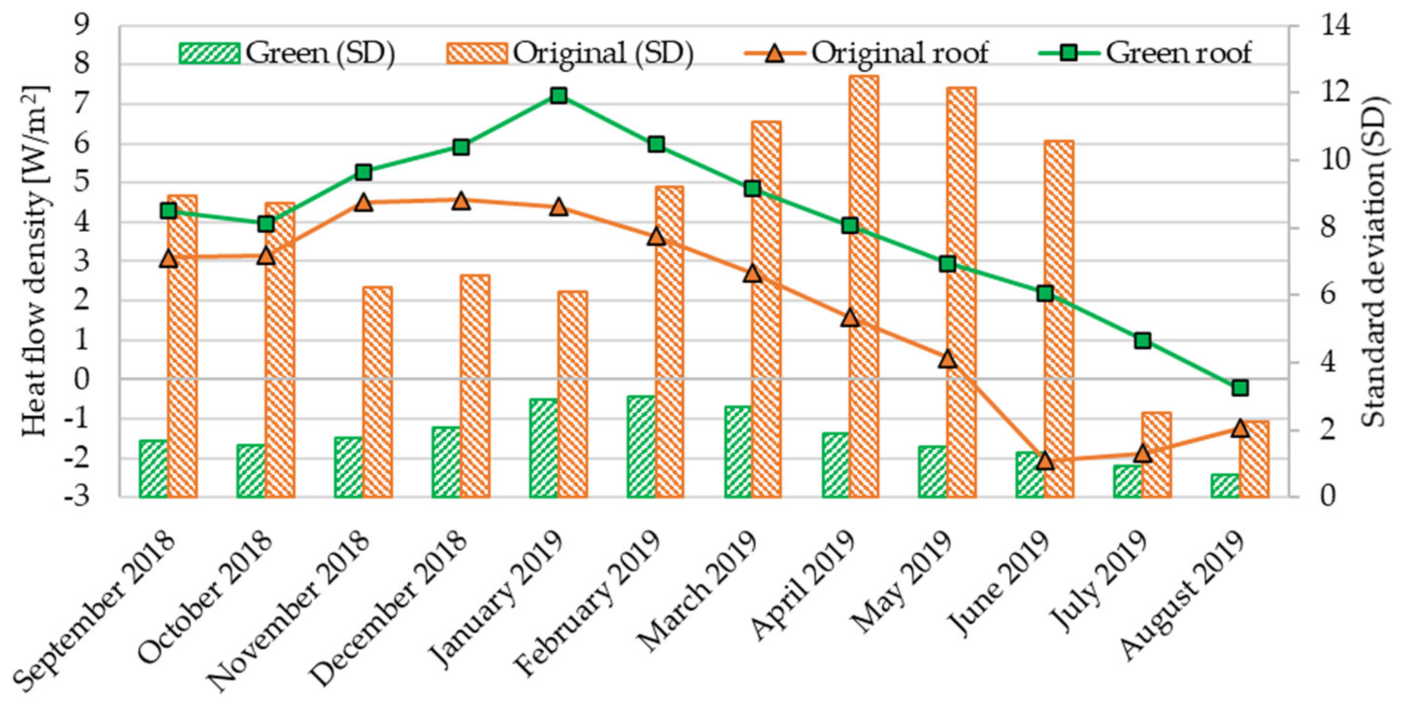
Figure 3 shows the average values of the heat flow densities and their SDs. The average monthly heat flow densities are represented in the graph by continuous lines on the main axis: the green curve is relative to the green roof (indicated in the legend with “Green roof”), while the orange one refers to the original roof (indicated with “Original roof”).

In the secondary axis, the monthly SD of the heat flow are represented: the green columns are relative to the green roof (indicated by “Green (SD)”), while the orange ones are relative to the original roof (“Original (SD)”).

The analysis of the heat flow densities reveals low average values for the original roof, but it is worthy to note that it is characterized by SD values always higher than those related to the green roof. Therefore, when compared with the original one, a stable thermal performance of the green roof can be observed. Taking into consideration December 2018 (representative of the winter season), the external air temperatures ranged between 3.83 °C and 14.16 °C. Throughout this month, the highest heat flux value was about 14 W/m², much lower than that recorded for the original roof (with a heat flux higher than 18 W/m²). The low thermal inertia of the original roof revealed a strong heat fluxes oscillation, also with negative values. The greater inertial effects of the roof-lawn system can be observed even more clearly during the middle season (from March 2019 to April 2019). Taking into consideration April 2019, the external air temperatures ranged between 5.53 °C and 26.23 °C. For the green roof, a maximum heat flux of about 10.7 W/m² was recorded. On the other hand, a maximum heat flow value of about 19.1 W/m² was registered for the original roof.

During the summer season, considering June 2019 as a representative month, the external air temperatures varied between 16.0 °C and 33.4 °C. In this month, for the green roof, the highest heat flux was about 6 W/m². Conversely, for the original roof, the highest heat flow was about 15 W/m². In order to provide an overview,

Table 3. Average, minimum and maximum heat fluxes registered during each month. The convention used is positive flux in the outgoing direction and negative flux in the inward direction.

Case 1	Green Roof—Heat Flux (W/m2)			Original Roof—Heat Flux (W/m2)
	MIN	AVG	MAX	MIN	AVG	MAX
September 2018	1.38	1.69	9.05	−21.02	3.11	8.95
October 2018	1.26	3.97	10.21	−18.06	3.16	18.54
November 2018	1.94	5.27	12.01	−11.88	4.52	19.01
December 2018	2.01	5.91	14.30	−10.42	4.56	19.61
January 2019	2.57	7.23	14.25	−10.15	4.39	14.80
February 2019	1.37	5.97	14.59	−23.61	3.64	19.52
March 2019	0.20	4.84	13.79	−25.38	2.71	20.13
April 2019	1.48	3.92	10.66	−32.56	1.59	19.07
May 2019	1.01	2.95	8.47	−29.17	0.54	17.81
June 2019	−0.61	2.20	5.59	−33.79	−2.06	15.04
July 2019	−0.19	0.99	5.36	−7.63	−1.87	2.38
August 2019	−3.69	−0.22	1.16	−6.47	−1.24	2.57

summarizes the average, the minimum and the maximum heat fluxes registered during each month.

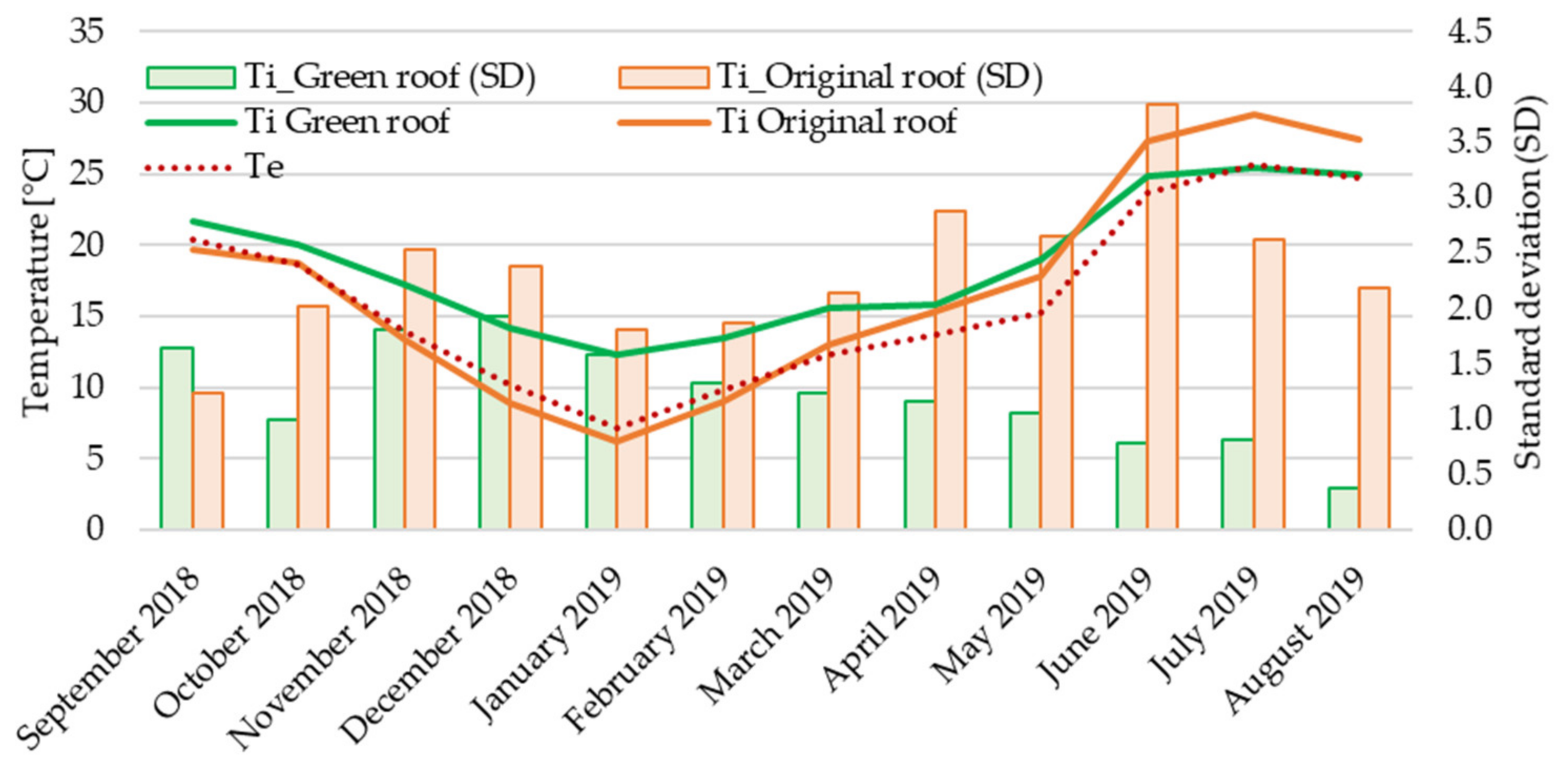
The average outdoor air temperatures, the average indoor air temperatures and their SD are reported in Figure 4.

The monthly average indoor air temperatures are represented in the graph by continuous lines on the main axis: the green curve is relative to the green roof (indicated in the legend with “T_i Green roof”) while the orange one refers to the original roof (indicated with “T_i Original roof”). On the main axis, the red dashed curve of the outside air temperature (indicated with “T_e”) is also represented.

The secondary axis shows the monthly SDs of the monthly indoor air temperature: the green columns refer to the green roof (indicated by “T_i_Green (SD)”), while the orange ones refer to the original roof (“T_i_Original (SD)”).

The constant thermal behavior of the green roof can be deduced also by observing the average internal air temperatures (Figure 4). From September 2018 to May 2019, they are always characterized by higher values when compared with the average indoor air temperatures of the original roof. On the contrary, during June, July and August 2019 the indoor air temperatures are lower than those registered for the original roof, with subsequent advantages in terms of indoor thermal comfort. Furthermore, in this case, SDs calculated for the original roof are greater than those computed for the roof equipped with the roof-lawn system. The behavior of the green roof is related both to the additional thermal resistance caused by the additional layer represented by the roof-lawn system and to the increased thermal inertia. Indeed, considering December 2018, the green roof caused an average indoor air temperature of 14.14 °C. Conversely, for the original roof, indoor air temperature showed an average value of 8.95 °C. During the middle season (April and May 2019) the average indoor air temperatures are similar, but it is possible to observe better performance with the roof-lawn system; during April 2019, a minimum internal air temperature of 13.91 °C caused by the green roof, and a minimum value of 9.52 °C caused by the original roof were obtained. Moreover, for the indoor air temperatures, aiming at providing an outline,

Table 4. Average, minimum and maximum indoor air temperatures registered during each month.

Case 1	Green Roof—Air Temperature (°C)			Original Roof—Air Temperature (°C)
	MIN	AVG	MAX	MIN	AVG	MAX
September 2018	19.6	21.7	24.2	17.7	19.7	22.5
October 2018	17.3	20.0	21.5	13.0	18.8	23.0
November 2018	13.7	17.2	20.6	7.2	13.4	18.3
December 2018	10.2	14.1	17.2	4.1	9.0	13.7
January 2019	10.0	12.4	15.6	3.9	6.2	9.9
February 2019	9.9	13.5	16.3	4.3	9.0	132.0
March 2019	12.8	15.6	19.2	7.1	13.0	18.1
April 2019	13.9	15.8	19.0	9.5	15.4	24.6
May 2019	16.2	19.0	22.2	10.9	17.9	24.4
June 2019	23.1	24.8	26.7	15.9	27.3	35.3
July 2019	23.7	25.5	27.5	23.4	29.2	34.8
August 2019	24.2	25.0	25.7	24.1	27.4	31.6

recaps the average, the minimum and the maximum values registered during each month.

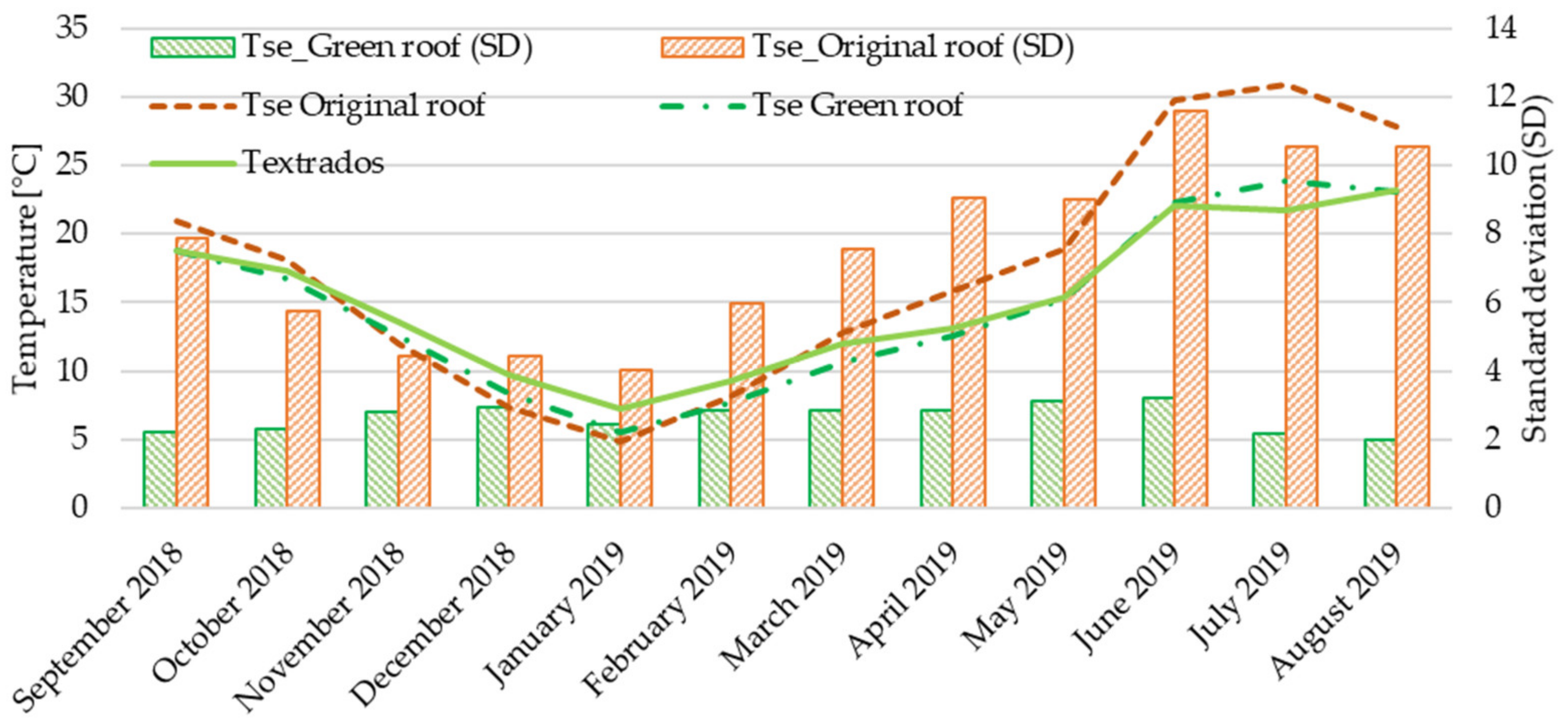
Finally, the average external surface temperatures and their SDs are shown in Figure 5, along with the extrados’ average temperatures measured under the roof-lawn system. The monthly average temperatures of the external surface are represented in the graph by dashed curves on the main axis: the green curve is relative to the green roof (indicated in the legend with “T_se Green roof”), while the brown one refers to the original roof (indicated with “T_se Original roof”). On the main axis, the green continuous curve of the extrados’ temperature is also shown (indicated by “T_exstrados”).

The secondary axis shows the monthly SDs of the external surface temperatures: the green columns are related to the green roof (denoted by “T_se_Green (SD)”), while the orange ones are related to the original roof (“T_se_Original (SD)”).

The outer side of the investigated roofs is completely different in terms of materials and heat transfer mechanisms. The effect of the thermophysical features of the employed materials played an essential role. The tiles on the original roof absorbed solar radiation because of their high absorptance coefficient. For the green roof, this did not happen because of the evapotranspiration phenomena of the greenery. Moving from the colder months to the warmer ones, it is possible to observe much higher average external surface temperatures in the case of the original roof. Analyzing the summarizing data listed in

Table 5. Average, minimum and maximum external surface temperatures registered during each month.

Case 1	Green Roof—Surface Temp. (°C)			Original Roof—Surface Temp. (°C)
	MIN	AVG	MAX	MIN	AVG	MAX
September 2018	12.0	18.8	24.0	8.2	20.9	42.2
October 2018	5.3	16.7	21.4	7.1	18.1	35.5
November 2018	5.7	12.5	18.4	1.5	12.0	23.4
December 2018	2.3	8.4	13.9	-2.4	7.4	17.8
January 2019	2.3	5.6	11.5	-2.5	4.8	15.8
February 2019	-0.5	7.7	14.1	-2.9	8.1	24.4
March 2019	0.7	10.7	18.6	-0.9	12.8	35.1
April 2019	6.4	12.6	21.4	2.5	15.9	42.7
May 2019	7.4	15.3	23.6	3.8	18.9	43.7
June 2019	13.3	22.3	28.8	8.9	29.7	52.9
July 2019	18.4	23.9	30.3	16.0	30.9	55.0
August 2019	20.4	23.1	27.1	16.5	27.8	49.5

, the original roof reached about 55 °C, while the external temperatures of the roof-lawn system reached values which do not exceed about 30 °C.

The recorded data during winter allowed the calculation of the U-value of the roofs. For the green roof, a U-value of 1.361 W/(m²K) was found and, for the original one, a value of 3.021 W/(m²K) was obtained. Thus, making a comparison between the roofs, a percentage difference in terms of thermal transmittance of about −55% can be pointed out. Moreover, applying Equation (3), the thermal conductance of the roofs was computed, finding 1.168 W/m²K for the green roof and 2.811 W/m²K for the original one, with a resulting percentage difference of −58.45%. The measurement of the green roof extrados’ temperature and the external surface temperature allowed a preliminary calculation of the roof-lawn thermal conductance, which was equal to 4.487 W/m²K. All these results are summarized in

Table 6. Case 1: C-values and U-values of the original and green roofs.

Case 1	Thermal Conductance (W/m2K)	Thermal Transmittance (W/m2K)
Original roof	2.811	3.021
Green roof	1.168	1.361
Roof-lawn	4.487	-

.

3.2. Case 2—Experimental Investigation

The experimental results of Case 2 are reported in this section. Again, the results of a one-year monitoring are presented here in terms of average data and SDs. Therefore, it is possible to make a direct comparison between the green roof and the original roof over time, also observing the fluctuations of the individual quantities on a monthly basis. From May 2019 to May 2020, it is possible to comprehend the thermal behavior of the green roof under different weather conditions.

It is necessary to specify that this monitoring has some missing data caused by the malfunction of the installed sensors.

Figure 6, Figure 7 and Figure 8 show the comparison between the green roof and the original one.

Figure 6 shows the average values of the heat flow densities and their SDs.

The average monthly heat flow densities are represented in the graph by continuous lines on the main axis: the green curve is relative to the green roof (indicated in the legend with “Green roof”), while the orange one refers to the original roof (indicated with “Original roof”).

In the secondary axis, the monthly SDs of the heat flow are represented: the green columns are relative to the green roof (indicated by “Green (SD)”), while the orange columns are relative to the original roof (“Original (SD)”).

The analysis of the heat flow densities reveals low average values for the original roof, but it is important to note that it is characterized by SD values always higher than those related to the green roof.

The greater inertial effects of the roof-lawn system can be observed even more clearly during the middle season. Taking into consideration May 2019, the external air temperatures ranged between 12.58 °C and 25.77 °C. For the green roof, a maximum heat flux of about 1.33 W/m² was recorded. On the other hand, a maximum heat flow value of about 2.88 W/m² was registered for the original roof. Taking into consideration May 2020, the external air temperatures ranged between 13.82 °C and 34.53 °C. For the green roof, a maximum heat flux of about 2.66 W/m² was recorded. On the other hand, a maximum heat flow value of about 3.06 W/m² was registered for the original roof.

During summer, considering June 2019 as a representative month, the external air temperatures ranged from 14.06 °C to 37.99 °C. In this month, for the green roof, the highest heat flux was about 2.38 W/m². Conversely, for the original roof, the highest heat flow was about 4.0 W/m².

In order to provide an overview,

Table 7. Average, minimum and maximum heat fluxes registered during each month. The convention used is positive flux in the outgoing direction and negative flux in the inward direction. Instrument failure caused missing data.

Case 2	Green Roof—Heat Flux (W/m2)			Original Roof—Heat Flux (W/m2)
	MIN	AVG	MAX	MIN	AVG	MAX
May 2019	−0.84	0.18	1.33	−1.96	−0.40	2.88
June 2019	0.13	1.04	2.38	−4.13	−1.25	4.00
July 2019	0.24	1.39	3.09	−5.18	−2.28	3.36
August 2019	−	−	−	−4.88	−2.00	3.81
September 2019	−	−	−	−3.65	−0.63	6.06
October 2019	−2.17	0.52	1.99	−3.91	−0.36	4.11
November 2019	−1.84	0.26	1.65	−1.58	0.53	4.00
December 2019	−3.04	−0.33	1.39	−1.77	1.17	5.20
January 2020	−3,82	−1.12	1.27	−1.21	1.89	6.10
February 2020	−2.89	−0.29	1.87	−3.65	0.92	5.27
March 2020	−1.46	0.05	1.65	−3.61	−0.16	4.04
April 2020	−2.17	−0.26	0.79	−2.97	−0.26	4.56
May 2020	−2.29	0.21	2.66	−2.15	−0.71	3.06

summarizes the average, the minimum and the maximum heat fluxes registered during each month.

Comparing the green and the original roofs, a more stable thermal performance of the green roof can be observed. Taking into consideration December 2019 (representative of the winter season), the external air temperatures ranged between 2.42 °C and 19.23 °C. Throughout this month, the highest heat flux was about 1.39 W/m², a much lower value than that recorded for the original roof (with a heat flux higher than 5.20 W/m²). The low thermal inertia of the original roof allowed us to observe a strong heat flows oscillation, also showing negative values.

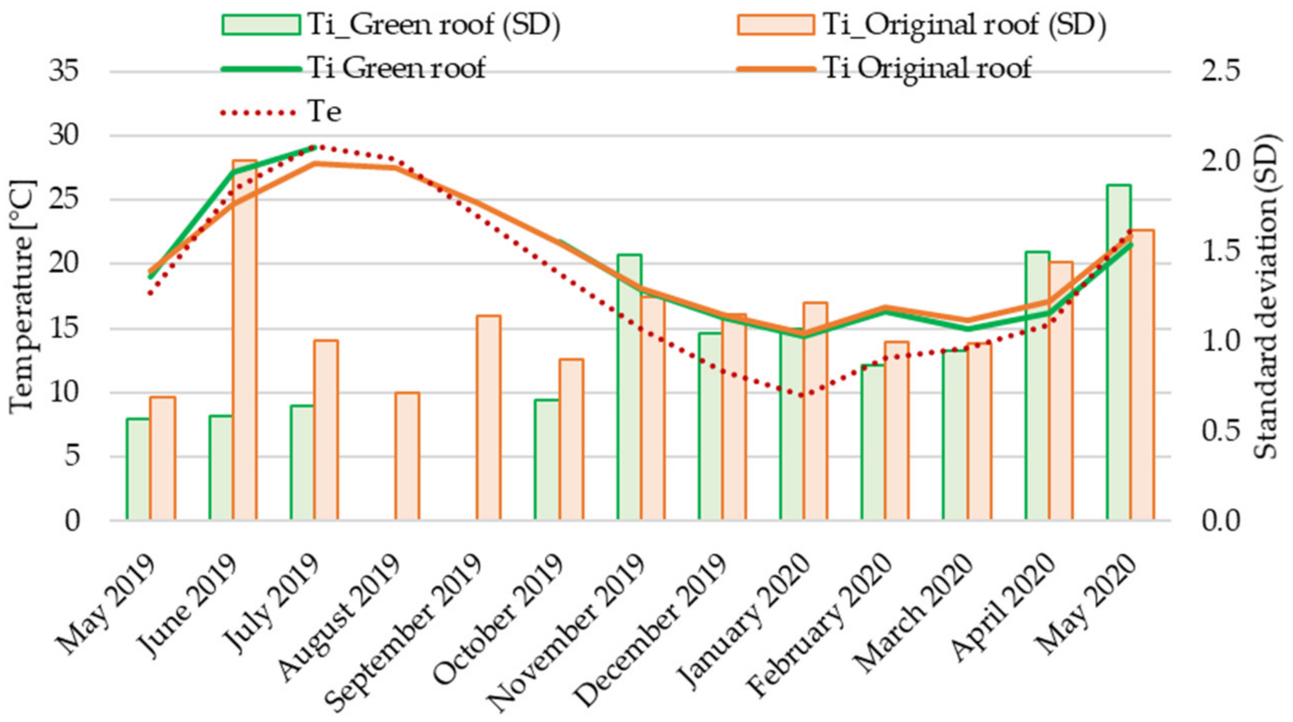
The average outdoor air temperatures, the average indoor air temperatures and their SDs are reported in Figure 7. The monthly average indoor air temperatures are represented in the graph by continuous lines on the main axis: the green curve is relative to the green roof (indicated in the legend with “T_i Green roof”), while the orange one refers to the original roof (indicated with “T_i Original roof”). On the main axis, the red dashed curve of the outside air temperature (indicated with “T_e”) is also represented.

The secondary axis shows the monthly SDs of the monthly indoor air temperature: the green columns refer to the green roof (indicated by “T_i_Green (SD)”), while the orange ones refer to the original roof (“T_i_Original (SD)”).

The more stable thermal behavior of the green roof can be deduced also observing the average indoor air temperatures (Figure 7). From May 2019 to May 2020, indoor air temperatures’ SDs calculated for the original roof are greater than those computed for the roof equipped with the roof-lawn system, except for November 2019 and for April and May 2020. In this case, the behavior of the green roof is also related both to the additional thermal resistance caused by the additional layer represented by the roof-lawn system and to the increased thermal inertia. Indeed, considering December 2019, the green roof caused an average indoor air temperature of 16.08 °C. On the contrary, for the original roof, an average indoor air temperature of 15.82 °C can be observed. During the middle season (April and May 2020) the average indoor air temperatures are similar: during April 2020, a minimum internal air temperature of 12.81 °C caused by the green roof, and a minimum value of 13.51 °C caused by the original roof were obtained. Additionally, for the indoor air temperatures, aiming at providing an outline,

Table 8. Average, minimum and maximum indoor air temperatures registered during each month. Instrument failure caused missing data.

Case 2	Green Roof—Air Temperature (°C)			Original Roof—Air Temperature (°C)
	MIN	AVG	MAX	MIN	AVG	MAX
May 2019	18.1	19.1	20.1	18.0	19.5	21.0
June 2019	26.0	27.2	28.2	18.9	24.7	27.7
July 2019	27.6	29.0	30.4	25.7	27.8	30.1
August 2019	-	-	-	26.3	27.5	30.2
September 2019	-	-	-	22.5	24.8	27.8
October 2019	20.0	21.7	23.2	19.8	21.7	24.5
November 2019	15.7	18.0	21.4	16.0	18.1	21.3
December 2019	13.1	15.8	18.4	13.1	16.1	18.6
January 2020	12.0	14.4	17.0	12.1	14.6	17.7
February 2020	13.7	16.3	18.0	13.9	16.6	18.6
March 2020	13.0	15.0	17.7	13.5	15.6	18.8
April 2020	12.8	16.2	18.4	13.5	17.1	19.3
May 2020	18.1	21.6	25.0	19.0	22.2	25.8

recaps the average, the minimum and the maximum values registered during each month.

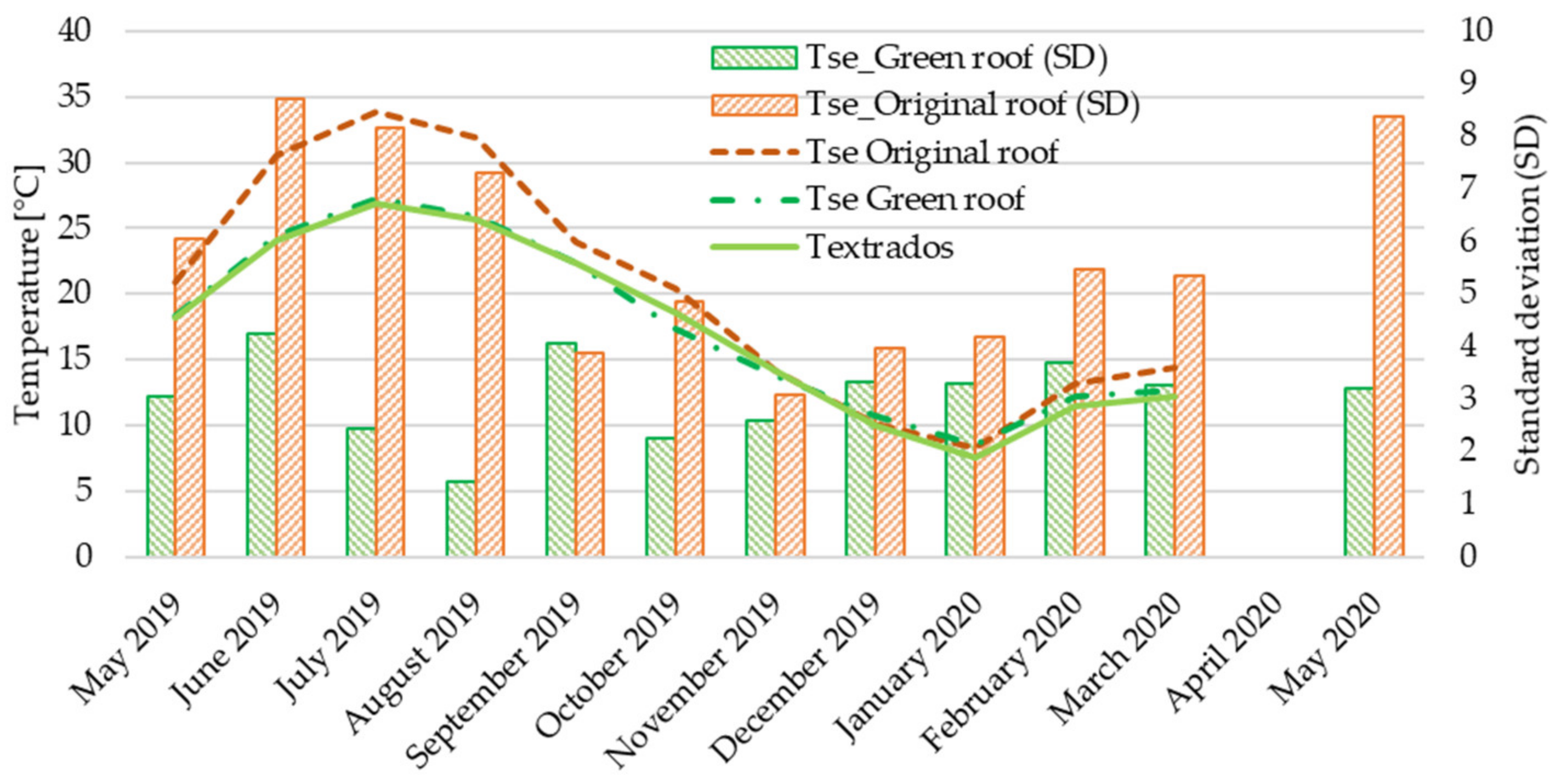
Finally, the average external surface temperatures and their SDs are shown in Figure 8 along with the extrados’ average temperatures measured under the roof-lawn system. The monthly average temperatures of the external surface are represented in the graph by dashed curves on the main axis: the green curve is relative to the green roof (indicated in the legend with “T_se Green roof”), while the brown one refers to the original roof (indicated with “T_se Original roof”). On the main axis, the green continuous curve of the extrados’ temperature is also shown (indicated by “T_exstrados”).

The secondary axis shows the monthly SDs of the external surface temperatures: the green columns are related to the green roof (denoted by “T_se_Green (SD)”), while the orange ones are related to the original roof (“T_se_Original (SD)”).

The outer side of the investigated roofs is completely different in terms of materials and heat transfer mechanisms. The effect of the thermophysical features of the employed materials played an essential role. Indeed, while in the original roof cover the solar radiation was absorbed by the tiles due to their high absorption coefficient, this phenomenon does not occur in the green roof due to the evapotranspiration phenomena of the greenery. Moving from the colder months to the warmer ones, it is possible to observe much higher average external surface temperatures in the case of the original roof. Analyzing the summarizing data listed in

Table 9. Average, minimum and maximum external surface temperatures registered during each month. Instrument failure caused missing data.

Case 2	Green Roof—Surface Temp. (°C)			Original Roof—Surface Temp. (°C)
	MIN	AVG	MAX	MIN	AVG	MAX
May 2019	13.3	18.3	30.1	13.2	20.8	45.7
June 2019	14.4	24.4	37.3	13.8	30.5	52.8
July 2019	22.3	27.2	34.0	21.7	33.9	54.3
August 2019	22.9	25.9	31.3	22.9	32.0	53.9
September 2019	15.1	22.4	40.0	19.6	23.9	45.6
October 2019	12.1	17.4	24.5	13.5	20.4	35.4
November 2019	8.2	13.8	20.5	8.4	14.2	26.2
December 2019	2.4	10.7	19.0	0.2	16.1	20.6
January 2020	2.1	8.6	17.5	0.5	10.1	22.5
February 2020	2.8	12.2	21.4	1.5	13.2	31.2
March 2020	7.2	12.7	28.3	6.2	14.4	33.2
April 2020	-	-	-	-	-	-
May 2020	12.9	19.5	31.0	12.0	25.9	48.8

, the original roof reached about 54 °C, while the external temperatures of the roof-lawn system reached values which do not exceed about 40 °C.

The recorded data during winter allowed for the calculation of the thermal transmittance of the roofs. Applying Equation (2), a U-value of 0.190 W/(m²K) was obtained for the green roof, and a value of 0.362 W/(m²K) was found for the original one. Therefore, making a comparison between the green and the original roof, a percentage difference in terms of thermal transmittance of about −47.5% can be highlighted. Moreover, applying Equation (3), the thermal conductance of the roofs was computed, finding a value of 0.162 W/m²K for the green roof and a value of 0.277 W/m²K for the original one, with a resulting percentage difference of −41.4%. The measurement of the green roof extrados’ temperature and the external surface temperature allowed a preliminary calculation of the roof-lawn thermal conductance, which was equal to 0.423 W/m²K. All these results are summarized in

Table 10. Case 2: C-values and U-values of the original and green roofs.

Case 2	Thermal Conductance (W/m2K)	Thermal Transmittance (W/m2K)
Original roof	0.277	0.362
Green roof	0.162	0.190
Roof-lawn	0.423	-

.

3.3. Building Energy Simulation

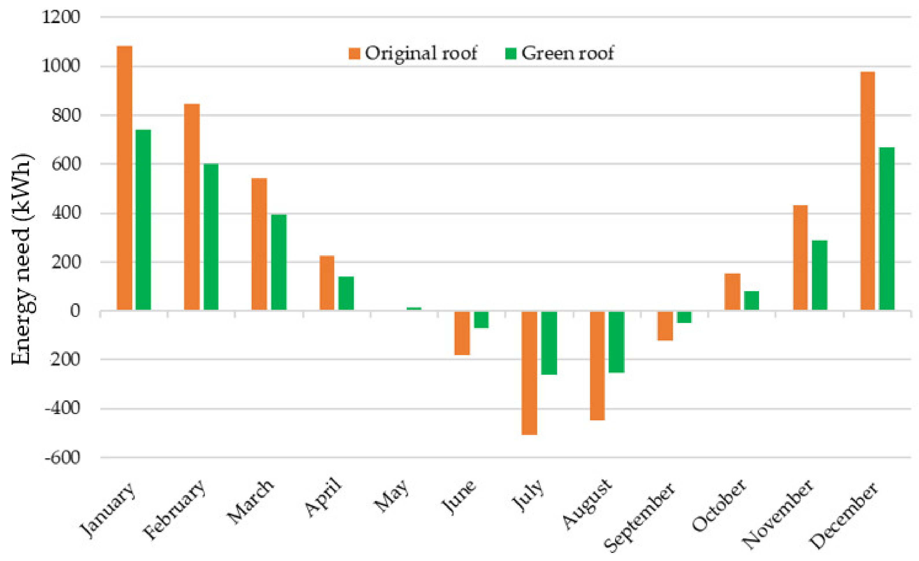
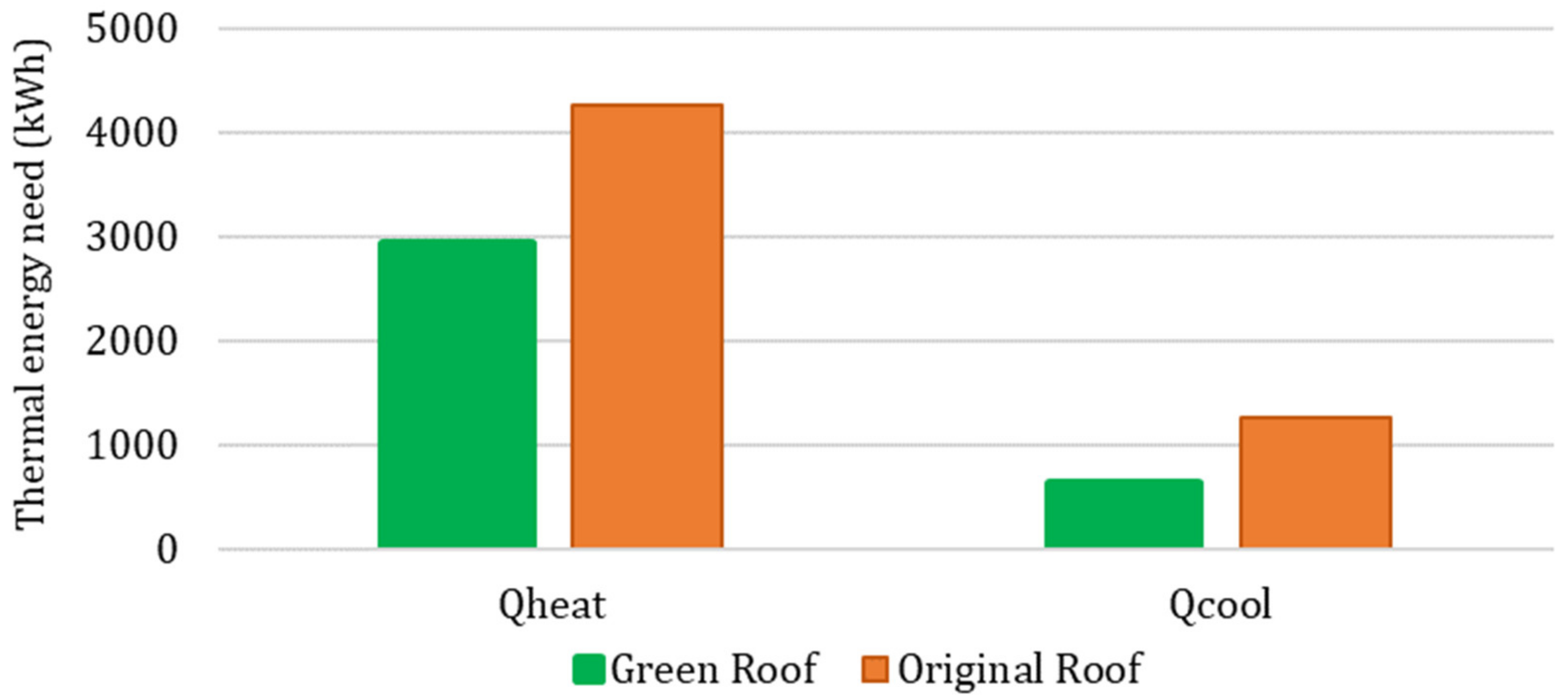
A dynamic energy simulation was performed in DesignBuilder in order to simulate the performance of the green roof. The resulting effects deriving from the installation of the green roof are shown in Figure 9, Figure 10 and Figure 11. In particular, Figure 9 shows the monthly thermal energy requirement of the building, considering as positive the amount of energy that needs to be added in the internal spaces and negative the energy that has to be removed to guarantee comfortable conditions in summer. Comparing the monthly thermal heating and cooling requirements (see Figure 9), it is possible to observe a relevant reduction of peak values in summer and winter design months: in particular, we observed a percentage difference of −31% in January (−339 kWh) and of −48% in July (+224 kWh). Instead, on an annual basis, the installation of the green roof is able to decrease the thermal energy requirement by 31% during the heating season (from October to April) and by 50% during the cooling period (form June to September). It should be noted that the building is characterized by a good summer performance, even if the original roof has poor thermal behavior. This can be linked to the use of high reflective solar blinds, to avoid summer overheating in internal spaces, and of natural ventilation systems.

In addition, since the best performance of the green roof was found in summer, an evaluation of comfort conditions was performed using the indicator predicted mean vote (PMV Fanger) [37].

The PMV Fanger is equal to zero when thermal neutrality is reached, while the comfort zone is defined as the interval between the recommended PMV limits (e.g., −0.5 < PMV < + 0.5). The index is calculated from Fanger’s equations that are characterized by six input parameters: air temperature, mean radiant temperature, relative humidity, air speed, metabolic rate, and clothing insulation.

A typical summer week was chosen (from 10 August till to 17 August), and the hourly PMV Fanger index is plotted in Figure 11. As can be noted, the installation of the green roof is able to sensibly improve the comfort conditions during the working days, keeping the index in the range between −1 and +1. Since the air speed, metabolic rate and the clothing insulation are considered constant in the simulation, and the air temperature is controlled by the cooling system, the installation of the green roof results to improve the distribution of surface temperatures and the values of relative humidity in the building rooms during the analyzed period.

Analyzing the results deriving from the simulation model, it is possible to affirm that the installation of a green roof is able to reduce energy consumptions in both heating and cooling seasons due to its properties of insulation and thermal inertia. Furthermore, a sensible improvement of comfort conditions in the building’s internal spaces was found during the summer period.

4. Conclusions

This study aimed to investigate the thermal behavior of an innovative roof-lawn system, tested on two buildings placed in central Italy. Long-lasting measurement campaigns were carried out, and simulations were performed in order to understand the influence of this passive technique on the energy performance of buildings.

In both case studies, the green roof showed more stable thermal behavior, characterized by lower heat fluxes and temperature fluctuations. This is related to the additional massive layer represented by the roof lawn system, which influenced the steady state and the dynamic thermal performance of the roof.

For Case 1, the green roof showed a thermal transmittance of 1.361 W/(m²K), and the original one a value of 3.021 W/(m²K). Thus, comparing the green and the original roof, a percentage difference of about −55% was found. In terms of thermal conductance of the roofs, a value of 1.168 W/m²K for the green roof and a value of 2.811 W/m²K for the original one was identified, with a resulting percentage difference of about −58%. The measurement of the green roof extrados’ temperature and the external surface temperature allowed a preliminary calculation of the roof-lawn thermal conductance, which was equal to 4.487 W/m²K.

For Case 2, the green roof showed a thermal transmittance of 0.190 W/(m²K) and the original one a value of 0.362 W/(m²K). In this case, a percentage difference in terms of U-value of about −47.5% was found. Moreover, the thermal conductance of the roofs was computed, finding a value of 0.162 W/m²K for the green roof and a value of 0.277 W/m²K for the original one, with a resulting percentage difference of about −41%. In this case, the calculation of the roof-lawn thermal conductance was equal to 0.423 W/m²K.

The effects of the roof-lawn system in terms of annual energy needs were simulated by means of a dynamic code, achieving significant reduction in terms of heating and cooling energy demands. Simulating the roof-lawn system and making a comparison with the original roof, primary energy reductions of 30% for heating and 51% for cooling were obtained, respectively. Benefits were found considering indoor thermal comfort.

Since ancient times, green roofs have always been considered thermal insulators, representing a sustainable answer to the energy saving problem. Future developments of this study will regard the optimization of the green roof performance, focusing on the structural part of the roof, identifying a roof composition able to work better with the roof-lawn, and taking advantage of the thermophysical properties of the system. For this purpose, it would be interesting to carry out the prolonged monitoring of several case studies, considering different geographical areas and the orientations of other roofs, as well as the study of buildings with different areas, uses and occupancy rates.

A broader, transversal and complex study can lead to a more reliable estimation of both energy savings and comfort increase. Finally, a financial analysis could be included, investigating installation, operation and maintenance costs.