Article

Demand Flexibility Enabled by Virtual Energy Storage to Improve Renewable Energy Penetration

1
Department of Energy, Politecnico di Torino, 10129 Torino, Italy
2
Hypertech Energy Labs, Hypertech SA, 15232 Chalandri, Greece
*
Authors to whom correspondence should be addressed.
Energies 2020, 13(19), 5128; https://doi.org/10.3390/en13195128
Submission received: 26 August 2020 / Revised: 22 September 2020 / Accepted: 29 September 2020 / Published: 1 October 2020
(This article belongs to the Special Issue Energy Flows and Synergies between Energy Networks)

Abstract

:
The increasing resort to renewable energy distributed generation, which is needed to mitigate anthropogenic CO2 emissions, leads to challenges concerning the proper operation of electric distribution systems. As a result of the intrinsic nature of Renewable Energy Sources (RESs), this generation shows a high volatility and a low predictability that make the balancing of energy production and consumption difficult. At the same time, the electrification of new energy-intensive sectors (such as heating) is expected. This complex scenario paves the way for new sources of flexibility that will have more and more relevance in the coming years. This paper analyses how the electrification of the heating system, combined with an electric flexibility utilisation module, can be used to mitigate the problems related to the fluctuating production of RES. By using Power-to-Heat (P2H) technologies, buildings are able to store the overproduction of RES in the form of thermal energy for end-use according to the principle of the so-called Virtual Energy Storage (VES). A context-aware demand flexibility extraction based on the VES model and the flexibility upscale and utilisation on district-level through grid simulation and energy flow optimisation is presented in the paper. The involved modules have been developed within the PLANET (PLAnning and operational tools for optimising energy flows and synergies between energy NETworks) H2020 European project and interact under a unified co-simulation framework with the PLANET Decision Support System (DSS) for the analysis of multi-energy scenarios. DSS has been used to simulate a realistic future energy scenario, according to which the imbalance problems triggered by RES overproduction are mitigated with the optimal exploitation of the demand flexibility enabled by VES.

1. Introduction

It is well known that the mean global temperature has been increasing over the last and present century due to anthropogenic emissions [1] and, if no countermeasures are defined, this will lead to permanent environmental upheavals on the planet [2] As stipulated in the Paris Agreement [3] in 2015, and then formalised in the “Clean Energy for all Europeans” legislation package in 2019 [4], decarbonisation of the power sector is one of the strategic policies that the European Union has defined in order to reduce the anthropogenic contribution to climate change; it has in fact been estimated that about 30% of the world’s Greenhouse Gas (GHG) emissions is produced by the power sector [5]. Renewable Energy Sources (RES), which are capable of providing energy with no emission costs, play a fundamental role in achieving such a goal [6]. For this reason, a marked increase in RES penetration and distributed generation can be expected in the near future. This, on one hand, will allow the GHG emissions related to electricity energy production to be reduced, while, on the other hand, it will create an imbalance of the grids related to the intermittent nature of the renewable sources. In fact, the current electrical system was not designed to manage bi-directional flows and variable generation patterns [7], and this can cause problems during the inevitable moments of uncontrolled energy overproduction. In order to tackle this problem, it is necessary to review the electricity grid management paradigm and find new sources of flexibility [8] and control methods [9] that are able to guarantee a continuous balance between production and consumption in the electrical network.
In parallel with the increase in RES penetration, it is expected that certain important energy-intensive sectors, such as mobility [10] and space heating [11], will move towards more sustainable systems powered by electricity. While these new electrical loads may aggravate the grid imbalances, at the same time they will offer new sources of power flexibility that can contribute to balancing the network. Energy conversion technologies (Power-to-X, P2X) can act as a connection between different energy sectors and allow advantage to be taken of the intrinsic flexibility of an integrated energy system in order to optimise energy flows in an electricity network [12]. For example, the heating/cooling needs of a building offer a certain degree of flexibility as the thermal response of the buildings is not immediate, given their thermal inertia properties. In cases of flexibility exploitation, the indoor temperature of a building may in fact vary over a pre-arranged range, which is estimated on the basis the inhabitants’ thermal comfort zones. If the buildings are equipped with stand-alone electrical heating/cooling systems, such as heat pumps, the flexibility of the thermal demand is reflected in the electrical demand flexibility of the devices.
Overall, VES-enabled demand flexibility is obtained from the thermal storage capabilities derived from the thermal inertia of a building, combined with electric-powered heating devices, while considering the comfort profiles of the building’s occupant. Several studies related to the impact of Virtual Energy Storage on smart grid integration and demand-side management can be found in the literature. Jin et al. (2016) [13] explored the VES concept, on the basis of a thermal equivalent model of a building space, using the internal–external temperature conditions and the thermal energy gains from natural and artificial heat sources as inputs. They calculated an optimal schedule for a constraint optimisation problem that considered contextual conditions related to the building envelope, the residents, the electricity price and the energy balance. Sikder and Jansson [14] studied pre-heating schemes, in terms of flexibility exploitation, to detect optimal VES management strategies in order to modulate the required demand without undermining the economic optimisation from the prosumer’s point of view. The explored scenarios were based on a self-consumption business case with time-of-use electricity prices related to the PV penetration levels throughout the day. The pre-heating strategies were modelled considering their duration and the final indoor temperature that they could achieve. The space thermal modelling was based on the electrical equivalent model approach, and a Bayesian engine was utilised for the estimation of the preferred indoor temperature. Asare et al. [15] performed a comparative economic analysis of the two main forms of residential energy storage, namely the “actual” storage achieved through electrochemical batteries and the virtual one realised through building thermal inertia. They concluded, from the experimental validation, that VES-enabled flexibility demonstrates better cost effectiveness at a residential scale, provided the pre-heating/cooling procedures are scheduled timely in order to avoid an overconsumption of electrical energy. The thus-obtained cost-effectiveness is related to the fact that demand time-shifting, through the VES technology, relies upon smart thermostat systems and gateways, which constitute a cheaper hardware solution than batteries and power converters.
However, only a few VES models have been presented in the literature, and the novelty of this paper is that it presents a new VES modelling approach. In general, VES models incorporate similar features to those of the current literature, with respect to space thermal modelling and any other related contextual conditions. Although the space thermal model is configured through a single thermal resistance and capacitance in many studies, the here described VES model distinguishes between the thermal dynamics of the wall and the air in the space for accuracy purposes. Accuracy is also guaranteed through the calibration of the model parameters, which is conducted using specific measurements and tests on real commercial and residential buildings. Furthermore, the model was designed in such a way as to allow the external control of the energy response of the VES technology, without violating internal comfort constraints. This paper shows how such a system can be integrated in a simulation platform of multi-energy energy systems and used to perform a district-level analysis, from the electrical distribution grid perspective, in order to capture the benefits of the VES-related demand flexibility for both an individual building and the whole district level. This architecture allows to simulate the demand flexibility from small-scale distributed loads (enabled by the VES approach) and to exploit it on district-level in order to optimise energy flows in the presence of high shares of renewable energy. In this work, two simplified control systems that optimise the electrical consumption of VES buildings at each simulation time-step are analysed and compared. The former refers to context-aware and comfort-preserving flexibility optimisation and the latter to network energy flow optimisation and coordination of the flexibility assets.
The VES model presented in this paper is realised within the PLANET (PLAnning and operational tools for optimising energy flows and synergies between energy NETworks) project [16], the objective of which is to analyse the possible synergies that can be derived from the coupling of different energy carriers (electricity, heat and natural gas), and to develop a Decision Support System (DSS) tool that allows interconnected sector scenarios to be simulated.
In the present study, the DSS tool is used to simulate a district electrical network template in which all the buildings are heated through Local P2H (LP2H) systems, and which also involves large PV installations that can cause energy overproductions. How the flexibility of the VES-enabled demand can be utilised optimally to the benefit of the local electrical network is also analysed.

2. Methodology and Tools

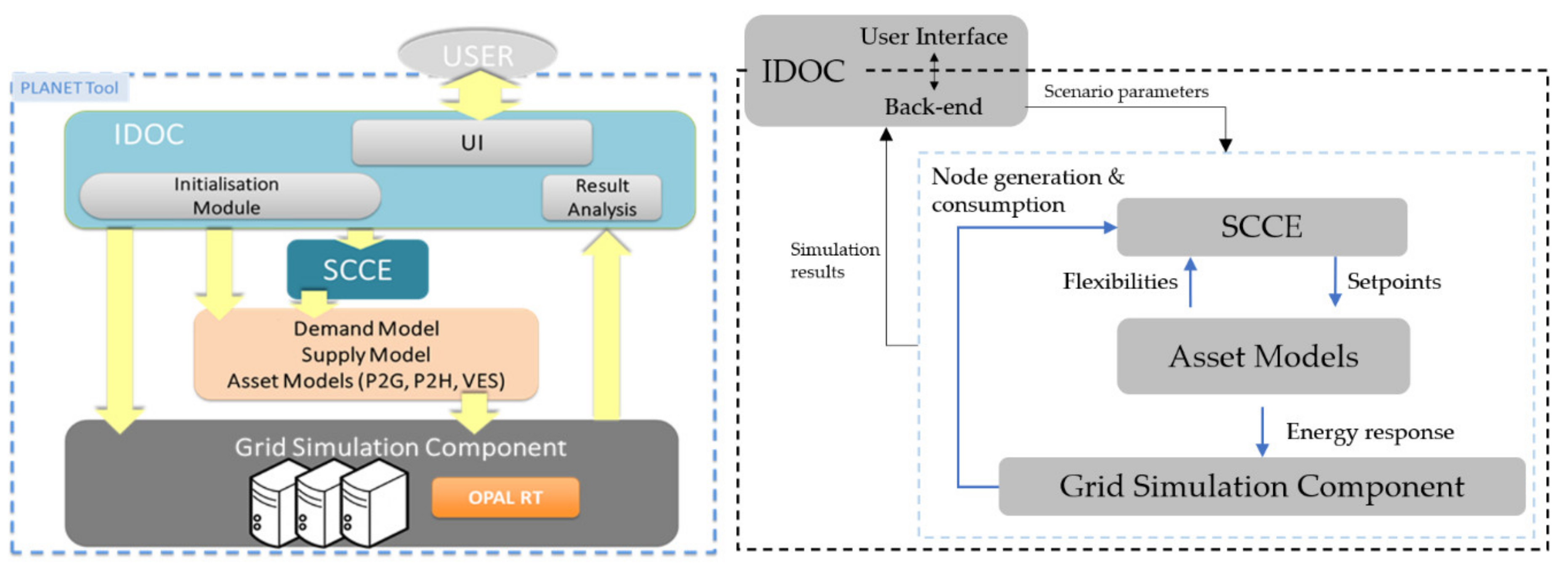
2.1. The PLANET DSS Tool

This work was carried out using the DSS tool developed as part of the PLANET project. PLANET DSS is an advanced computer tool that can be used to model multi-energy systems. The tool allows multi-energy system scenarios to be analysed at a district level, by simulating the energy flows and energy conversions, made possible thanks to energy P2X technologies, in their various forms (electricity, heat and natural gas). The flexibility provided by the energy conversion and storage units (P2H, P2G, VES) is exploited, in these complex scenarios, to improve the integration of distributed renewable energy generation in a multi-carrier coordination framework involving electricity, heat and natural gas networks [17] (see Figure 1).
The main inputs of the model are the capacity and distribution of renewable production plants, the energy demand (electricity, heat and natural gas), and the energy storage and conversion technologies installed within the analysed scenario. The results include the energy balance, the energy flows within the scenario, the share of RES, energy consumption, the RES over-production and the flexibility offered by the energy conversion and storage technologies.
The PLANET DSS tool is basically composed of four different modules [18] (see Figure 2):
  • The web User Interface (UI) and orchestration module: IDOC (Integrated Decision Support System and Orchestration Cockpit);
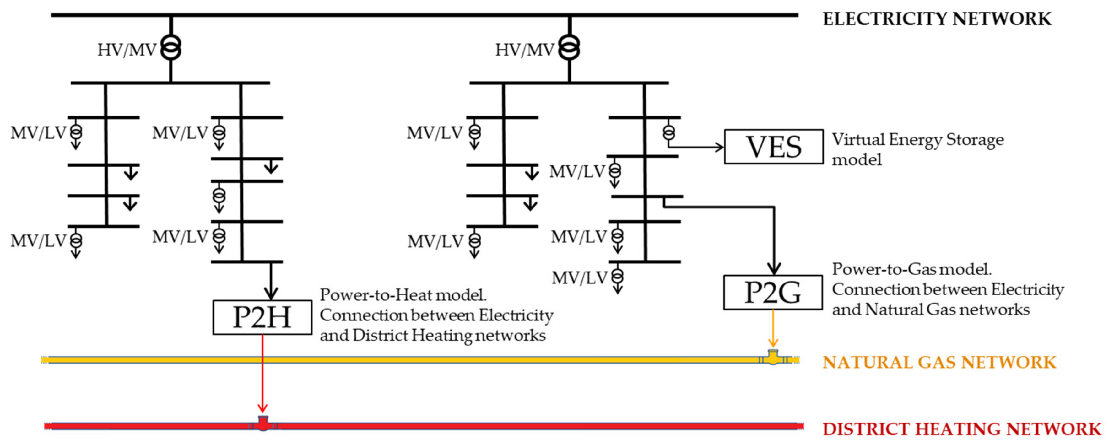
  • The energy conversion and storage asset models (P2G, P2H and VES);
  • The system optimisation module: SCCE (District-Level Storage/Conversion Coordination Engine);
  • The grid simulation component.
The tool is set up on a web platform with which the user can interact in order to perform remote simulations. The different modules are located in different remote machines, whose communication and synchronisation is conducted in a unified co-simulation framework [19]. This co-simulation structure makes the PLANET DSS very scalable and flexible, as each module can easily be replaced or modified in a plug and play fashion [20].
The user interacts with the DSS through the user interface (UI) part of the IDOC module (IDOC front end) with which he/she can define the scenario parameters (e.g., network parameters, demand and energy generation as well as the network connection of the energy conversion and storage technologies). The IDOC back-end functions dispatch the user-defined initialisation scenario parameters to the different modules and also retrieves and analyses the results at the end of the simulation. The result analysis is based on a series of KPIs, and is followed by result publishing and visualisation through the UI. The scenario, configured through the UI, is simulated for scalable time horizons (e.g., one day, one month, one year, etc.) and with a time discretisation (15 min, 1 h) in order to facilitate the analysis of different scenarios and impact assessment targets. The IDOC also has the task of coordinating and synchronising the information flows during the simulation that occurs between the other modules, as shown in Figure 2. The flexible asset module calculates the energy response of the assets on the basis of the status of the assets themselves and the operating parameters defined by the user. The asset modules also calculate the available flexibility, defined as the availability to modify the electric consumption (see Section 2.2.2). The grid simulation component receives the energy response of the assets and performs a power flow analysis within the analysed network. This module has been developed with the OPAL-RT eMEGAsim Power Grid simulator [21], which allows the behaviour of the power gird to be simulated with a good approximation (see also [22,23]). The SCCE controller receives the energy consumptions and generations from the grid simulation component and, according to the flexibility offered by the assets, defines the optimal operation set-points of the assets [24] (see Section 3).

2.2. Virtual Energy Storage (VES) as a Flexibility Asset

2.2.1. Virtual Energy Storage Technology within the PLANET Framework

The Virtual Energy Storage technology, which is based on controllable loads, provides flexibility extraction possibilities that can contribute to the management of the grid constraints, if run at an aggregated level. The modification of demand, attained through VES-enabled flexibility, with reference to a nominal baseline consumption, simulates battery operation during charging and discharging operations [25], thereby transforming a group of buildings into a district-level flexibility asset.
The PLANET framework includes VES as one of the storage/conversion technologies that can serve as key-enablers of network planning and system management, in order to support the core functions of a future DSO, such as enhanced demand-generation and network power flow forecasting, the local coordination of network configurations, [26] etc. Virtual Energy Storage introduces the demand-side management into the PLANET context, focusing on intra-building thermal loads, while incorporating a comfort-preserving approach to flexibility modelling.
The flexibility of the VES-enabled demand depends on two factors, namely the thermal properties of the building envelope and the usage patterns of its occupants and their comfort perception (e.g., space temperature, hot water availability, etc). The controlled variations of the baseline demand forecast through pre-heating/cooling techniques constitute the human-centric demand flexibility. The VES asset provides context-aware demand flexibility profiles that minimise or maximise the energy consumption time-series under certain constraints related to the thermal comfort boundaries and space thermal inertia, while taking into account any externalities that influence the indoor conditions, e.g., weather patterns, seasonality, etc.
The flexibility profiling was conducted at a building-level, and was followed by an aggregation process, given that the VES module provides the electrical response at a district level as input for network optimal planning. The VES portfolio comprises different types of buildings that correspond to residential and/or commercial consumers and provides the aggregated flexibility per MV/LV node of the electrical grid [17].
Load selection is required for an aggregated portfolio formation, and this is performed on the basis of an a priori load classification that is based on technical, market and contractual criteria. According to the type of flexibility-related service (e.g., balancing, wholesale, constraint management service, [27] etc.), flexible-load clusters can be utilised with different energy volumes, accumulated peak power, response characteristics, ramp rates, etc. A unique flexible-load cluster is assumed within the PLANET framework, given that distribution constraint management services, enabled by specific types of flexible loads related to electric heating and cooling, are investigated [28].

2.2.2. VES Model Description

The Virtual Energy Storage module configures thermal inertia models that reflect the thermal dynamics of a building and integrates them with electric heating/cooling equipment models, such as HVAC devices, Electric Water Heaters (EWH), etc., and with thermal comfort profiles in a unified optimisation framework. To this end, PLANET VES comprises a thermal comfort profiling engine, a space thermal module and an LP2H module, as shown in Figure 3.
The quantified temperature boundaries ( T c o m f u p , T c o m f d o w n ) of a “thermal comfort zone” were estimated by means of resident comfort modelling. Estimates of the thermal properties of the building and of the thermal energy requirements were obtained, with respect to external weather parameters, by means of space thermal modelling. Finally, the LP2H device modelling transforms the building thermal energy requirements into the electrical demand on the basis of the inferred conversion efficiencies (e.g., via the coefficient of performance for heat pumps) [28].
Thermal comfort inference is based on a Bayesian classifier model that is trained with sensing, metering and actuation data, which are obtained from devices that are installed in an occupant’s premises. Residents’ comfort represents the class variable in the Bayesian engine and it has three states, i 0 , 1 , 2 , corresponding to comfort, discomfort in heating and discomfort in cooling, while the indoor temperature is an independent variable [29]. A high-level view of the conditional probability formulation, according to the Bayes theorem, is presented hereafter:
P ( i | T i n ) = P i × P T i n | i P T i n ,   i 0 , 1 , 2
where i is the class variable, T i n is a feature, which, in this case, is actually the indoor temperature P ( i | T i n ) , i 0 , 1 , 2 stands for the posterior probability, P i is the prior probability, P T i n is the evidence and P ( T | i ) ,   i 0 , 1 , 2 is the likelihood function.
An appropriate dataset, comprising temperature and user actions on the electric heating/cooling devices, was gathered. After the pre-processing and configuration, which were based on a set of configurable rules for the ambient and actuation data, a series of implicit and explicit discomfort events were generated and correlated with the temperatures. In order to combine various event data (e.g., changes in the operational status or set-point temperatures of an LP2H device) with the contextual conditions (e.g., indoor temperature) and to effectively correlate them with comfort classification states, the comfort model calibration phase is a prerequisite for the deduction of appropriate temperature-classification pairing values, to allow concrete user comfort profiling [30,31].
The building envelope properties in the VES module are represented by a low-order thermal network that includes a set of “effective” resistances (R1, R2, R3) and capacitances (C1, C2) [32]. The 3R2C model refers to a thermal zone, which is a subset of the building and includes electric heating/cooling equipment and an independent indoor environmental management system [33,34]. The thermal behaviour of a thermal zone is represented by the dry bulb air temperature value, T i n d o o r , which is assumed to be uniform within the thermal zone, and the averaged wall temperature, T w a l l . The second-order model was chosen because it effectively represents the fast dynamics of the indoor air and the slow dynamics of the wall mass [35]. The resistance values and capacitance configuration parameters are determined through a parameter identification procedure that is based on data streams obtained from building sensing, metering and actuation equipment. For the present experiment, the abovementioned configuration parameters were defined, through calibration, in actual residential and commercial buildings located in a PLANET pilot site in France. The mathematical formulation of the thermal model of a building for a single zone is:
x ˙ t = A x t + B u t
y t = C x t
where, x t is the state vector, which includes the two space temperature variables [ T i n d o o r t , T w a l l t ] ; u t is a vector that includes the measured variables of the external temperature, the thermal gains from solar irradiance and the electric heating [ T e x t t , Q s o l a r t , Q h e a t t ] ; y t is the measured T i n d o o r t value; A and B are matrices that include the system configuration parameters, namely the conduction, convection and infiltration-related resistances (R1, R2, R3); the space air and wall capacitances (C1, C2); and the coefficients of the thermal energy source distribution to the space air and walls (p1, p2, p3, p4).
A = 1 R 2 C 2 1 R 3 C 2 1 R 2 C 2 1 R 2 C 1 1 R 1 C 1 1 R 2 C 1 ;   B = 1 R 3 C 2 p 1 C 2 p 3 C 2 1 R 1 C 1 p 2 C 1 p 4 C 1 ;   C = 1 0 ;
The number of residential and commercial buildings in the analysed scenarios was defined by the user according to the experiment needs, while the heat loss coefficient values (1/R1, 1/R2, 1/R3), the thermal capacitances (C1, C2) and the thermal distribution coefficients (p1, p2, p3, p4) were deduced through a training/calibration procedure for residential and commercial benchmark buildings in the PLANET pilot site in France (see Section 3). The same applies for T c o m f u p and T c o m f d o w n , which are the upper and lower comfort temperature boundaries. The thermal distribution coefficients p1 and p2 refer to the solar gains to the wall and air node, while p3 and p4 refer to the electric heating gains. To that end, the coefficient of performance (COP) of a heat pump is calculated through the following equation:
C O P = p 3 + p 4
The optimisation algorithm of VES calculates the minimum and maximum electrical consumption timeseries by incorporating the thermal comfort, the thermal inertia of the building and LP2H device model outputs as constraints. An outline of the flexibility optimisation algorithm [32] is provided in Table 1.
The upwards and downwards flexibility is calculated from the difference in the minimum and maximum consumption from the thermal demand baseline, and it indicates the demand modulation potential in an individualised, comfort-preserving manner. After discretisation, the mathematical formulation of the optimisation problem is presented through the following equations [32].
m i n / m a x c o n t r o l n = 1 N J p t n
s u b j e c t   t o   T comf down t n T b a n d T i n d o o r t n T comf up t n + T b a n d
T i n d o o r t 1 T w a l l t 1 = T i n d o o r , 1 T i n d o o r , 1
x t n + 1 = e A t s t e p x t n + A 1 e A t s t e p I   B u t n
t s t e p = t n + 1 t n
where J p is the variable that has to be optimised, which, in this case, is the energy consumption, t n   n = 1 , , N is the set of time points and t s t e p = t n + 1 t n , T i n d o o r t n is the indoor temperature, whose value at time point t1 is T i n d o o r , 1 , A, B, x and u are the matrices and vectors described above, and I is an identity matrix. After the calculation of the minimum and maximum consumption per time point from (6), the upwards and downwards flexibility per time point is derived by subtracting the baseline consumption from maximum and minimum consumption according to the following formulas:
P f l e x , u p = 0 ,                                                                               P b a s e t n P m a x t n   P m a x t n P b a s e t n ,         P b a s e t n < P m a x t n    
P f l e x ,   d o w n = 0 ,                                                                                   P b a s e t n P m i n t n P m i n t n P b a s e t n ,         P b a s e t n > P m i n t n  
The flexibility optimisation is a model-predictive control (MPC) algorithm that provides the demand flexibility per time step, through an iterative process over a finite forecast horizon, taking into account the control set-point applied in the prior time step. The plant state is sampled at the first step and the “demand modification” strategy is computed for a finite time horizon by the optimisation algorithm. After the initial step, the plant state is sampled once again, and the calculations are re-initiated for the current model state with the aim of producing a set of new control set-points and a revised forecasted state path. The prediction horizon keeps shifting forward in each iteration. According to research conducted so far, the aforementioned approach has displayed good results and accuracy [36].

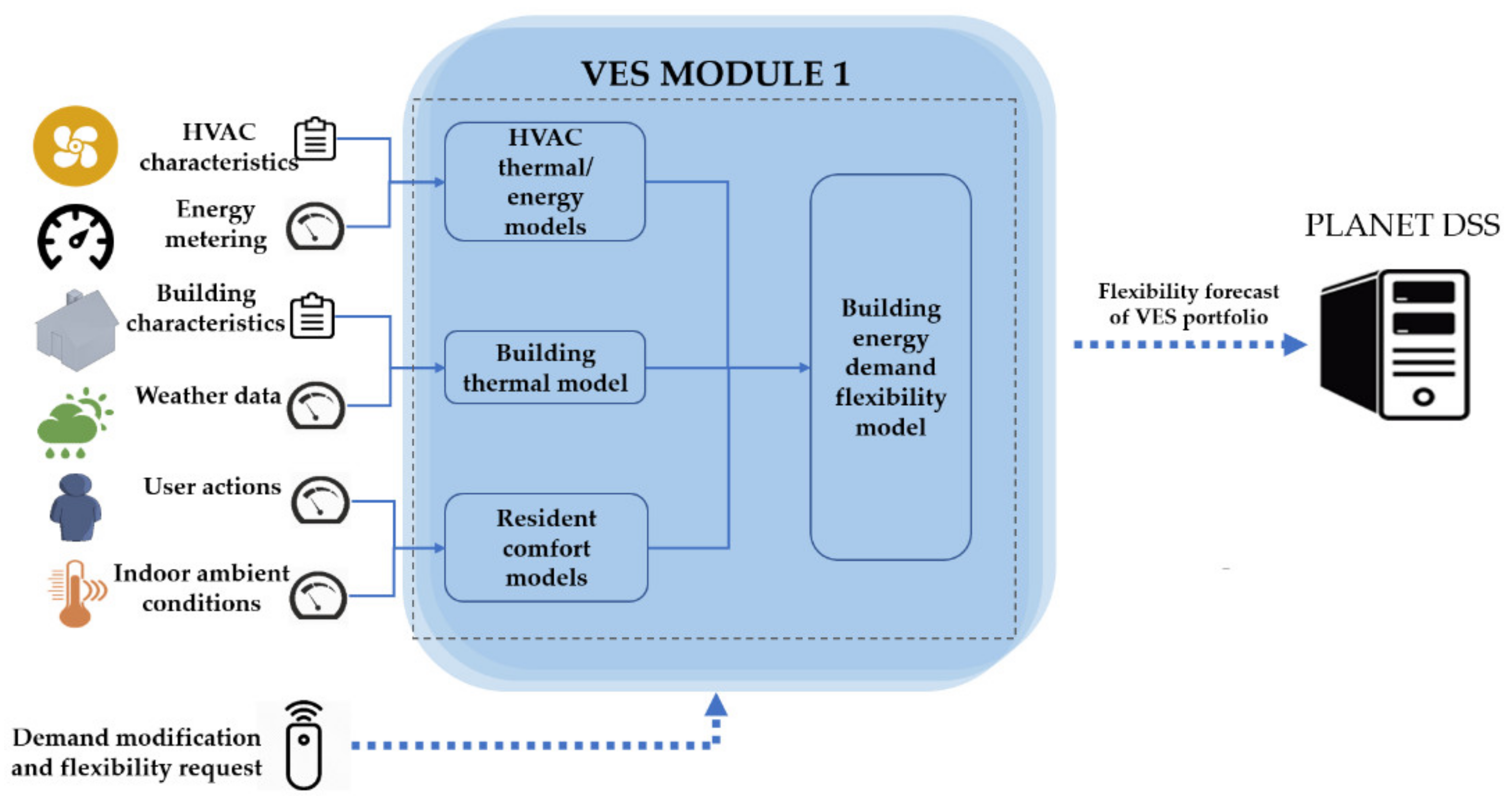
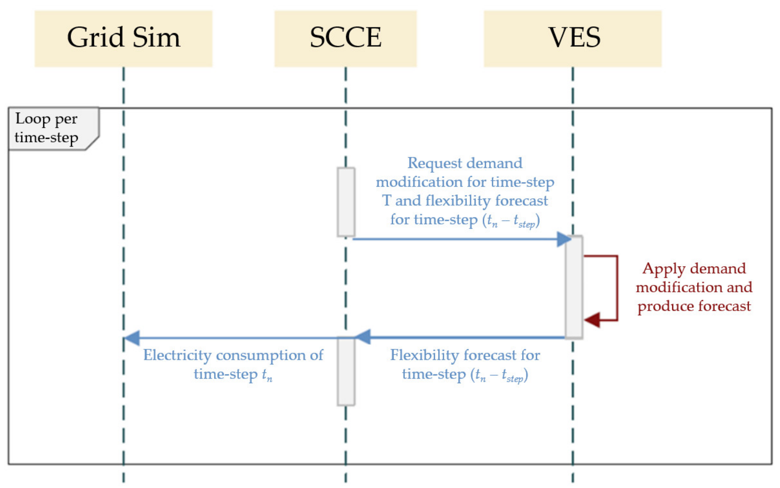
2.2.3. The VES Module: Architecture and Interfaces

PLANET VES represents an aggregated flexibility asset. A VES portfolio comprises a number of commercial and residential buildings, the configuration parameters of which are estimated along with the flexibility of the demand.
An aggregated VES portfolio is assigned to a combination of residential and commercial buildings. The configuration can be used for both operational planning case studies on pilot sites or more abstract simulations, in terms of sensitivity analysis.
The configuration parameters of the VES module are obtained from thermal comfort and space thermal model calibrations on data streams obtained from a pilot site in France (see Section 3). A VES portfolio, corresponding to an MV/LV grid node, provides an aggregated flexibility forecast to the Storage/Conversion management and Coordination Engine (SCCE), which performs an optimisation procedure on behalf of the electrical grid. After performing a global optimisation, SCCE returns the demand modification request for the current time-step to the VES module and requests a flexibility forecast for the next time step [19]. Figure 4 provides a holistic view of the information exchange architecture and the sequence of interactions of a VES module within the PLANET tool [28,37].
As indicated in Table 2, the flexibility forecast of the VES module comprises three different values: the baseline energy consumption, the downwards flexibility and the upwards flexibility. The demand modification requested by the SCCE should be within the boundaries set by the upwards and downwards flexibility. After the consumption is applied, an internal verification is performed in order to check whether the thermal comfort temperature boundaries are respected, and an acknowledgement is consequently dispatched to the SCCE, together with the updated flexibility forecast for the next time-step [38].

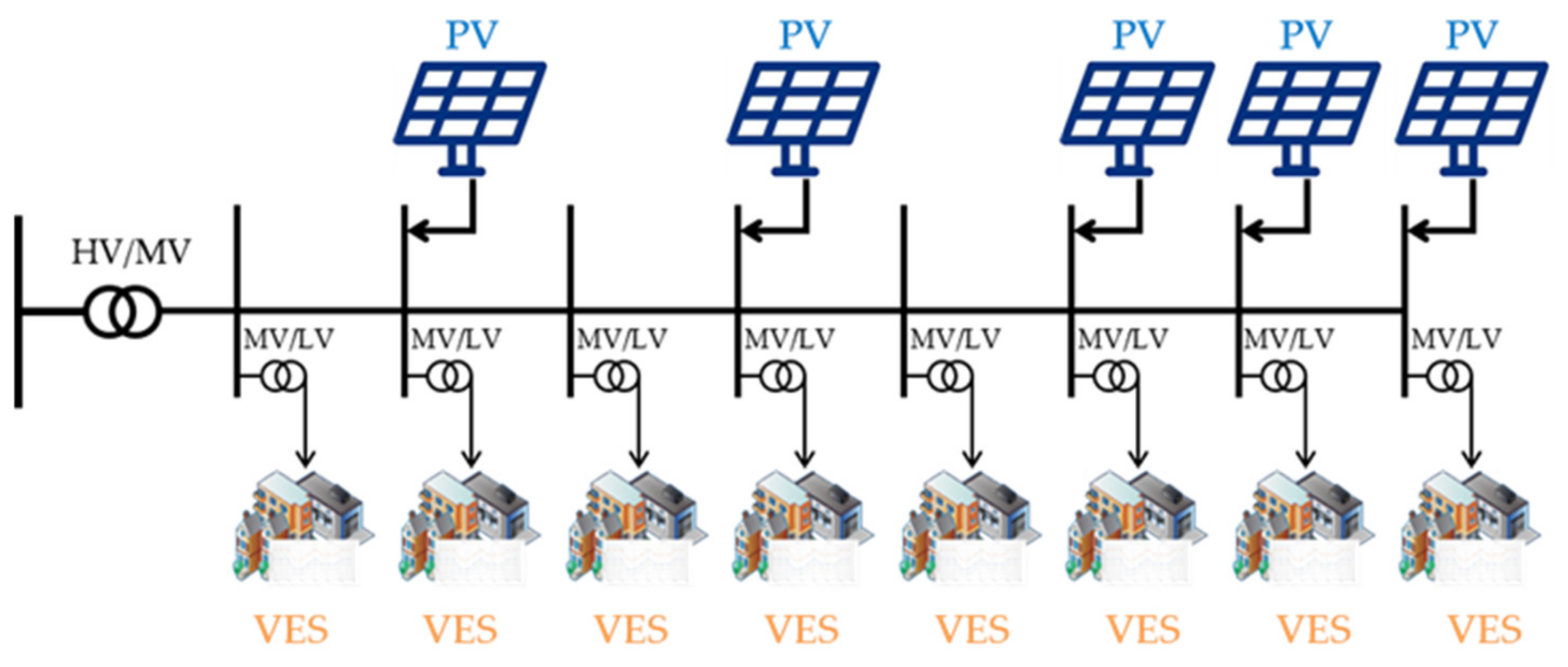
3. The Analysed Scenario

PLANET DSS was used to simulate a typical future high RESs energy scenario in order to evaluate the exploitation potential of VES-enabled demand flexibility for energy flow optimisation purposes. The grid template for the scenario set-up was created considering an eight-node medium voltage (MV) electric network that feeds a district with commercial and residential end-users. The buildings in the investigated district were considered to be equipped with the necessary infrastructure for VES-enabled flexibility profiling and forecasting (see Figure 5).
The distributed generation of the analysed district involved the use of photovoltaic (PV) plants. The technical information pertaining to the load and generation resources connected to each of the eight (8) nodes of the district grid template is reported in Table 3.
The commercial and residential buildings considered in the scenario were all equipped with electric heating systems (LP2H). These systems were hypothesised to have an electric nominal power of 4 kW for residential buildings and of 5 kW for commercial buildings. Table 3 includes two separate columns, one for the flexible LP2H-related load and the other for the rest of the fixed load connected to each grid node. The fixed load constitutes the electric consumption of all the end-users for each node that is uncontrollable. The fixed electricity consumption ( u n o d e   i ) for the i-th node was calculated with the following the formula:
u n o d e   i = b u i l d i n g s R E S   i   p u R E S   P f i x e d   R E S   i +   b u i l d i n g s C O M   i   p u C O M   P f i x e d   C O M   i
The residential end-user is associated with an uncontrollable load of 3 kW ( P f i x e d   R E S ) and the commercial one with 8 kW ( P f i x e d   C O M ). The b u i l d i n g s R E S   i and b u i l d i n g s C O M   i in Formula (1) represent the number of residential and commercial buildings, respectively, that are connected to the i-th node, while p u R E S and p u C O M are the per-unit consumption profiles of the residential and commercial consumers [39] (see Figure 6a).
The VES module was initialised on the basis of real data streams retrieved from sensing and metering equipment at the PLANET pilot site in the Maurienne Valley in France (see Section 3). Building automation equipment that enables ambient sensing and metering had been installed in a group of commercial and residential buildings in the town of Saint-Julien Montdenis, which is situated at about 600 metres above sea level in the South-East of France. To this end, a considerable amount of data were collected through customised gateways of benchmark buildings in the pilot site in order to be used as input in the demand flexibility profiling algorithms of the PLANET VES module during the calibration-initialisation phase.
Given the grey-box nature of the model, the initial VES calibration phase is actually an identification procedure that determines the maximum likelihood estimates of the adjustable configuration parameters that are presented in the respective part of Table 2. This function uses three different algorithms as alternative search methods in order to achieve the minimum error: the Gauss–Newton direction method, the Levenberg–Marquardt method and the steepest descent gradient search method. Several experiments were conducted under both free-floating conditions and with the P2H device in operation. Data from two (2) weeks of continuous sensing and metering were used as a minimum for each of the models. Furthermore, 30% of the dataset was utilised in all the calibration experiments to validate the accuracy of the trained model in the prediction of the space thermal dynamics. The metrics used to quantify and evaluate the performance of the model were the Root Mean Square Error (RMSE) and the level of fit (FIT).
The PV generation profiles were created on the basis of real measurements, provided by the local DSO-e, SOREA [40], combined with the ambient temperature profile for the same period and location, which was retrieved from the Renewable.ninja webiste [41] (see Figure 6b). The scenario was simulated during the winter season and in more detail throughout one full day at the beginning of March, with a time-step resolution of 15 min.
The control logic of the system was to optimise the demand flexibility provided by the VES-enabled buildings. The optimisation objectives at a district-level were the maximum absorption of RESs generation and the consequent balancing of demand and supply within the analysed scenario. The PV peak periods of a typical day contributed to an overproduction of the distributed generation resources and; therefore, to uncontrollable energy inflows in the local grid. If not regulated, this surplus creates a power flow from the distribution to the transmission grid, that is, the so-called Reverse Power Flow (RPF). Even though an RPF does not violate any voltage or current limits, it needs to be avoided, as the grid protection system is not designed to safely operate under such circumstances. Apart from the Reverse Power Flow phenomenon, it is of strategic importance for the local production to be consumed in a timely manner and at a local level in order to minimise transportation energy losses and the costly curtailment of distributed non-dispatchable generation.
To this end, the benefits of exploiting demand flexibility can be identified, in terms of local distribution network constraint verification and Reverse Power Flow, district-level self-balancing, with high shares of renewable penetration, and an overall energy efficiency. However, these objectives are not always combined simultaneously, since the absorption of surplus renewable production, through demand modulation schemes, is sometimes achieved to the detriment of energy efficiency. The following scenarios were simulated with three different optimisation strategies and control algorithms to investigate the value that VES-enabled flexibility offers to the local grid from multiple perspectives:
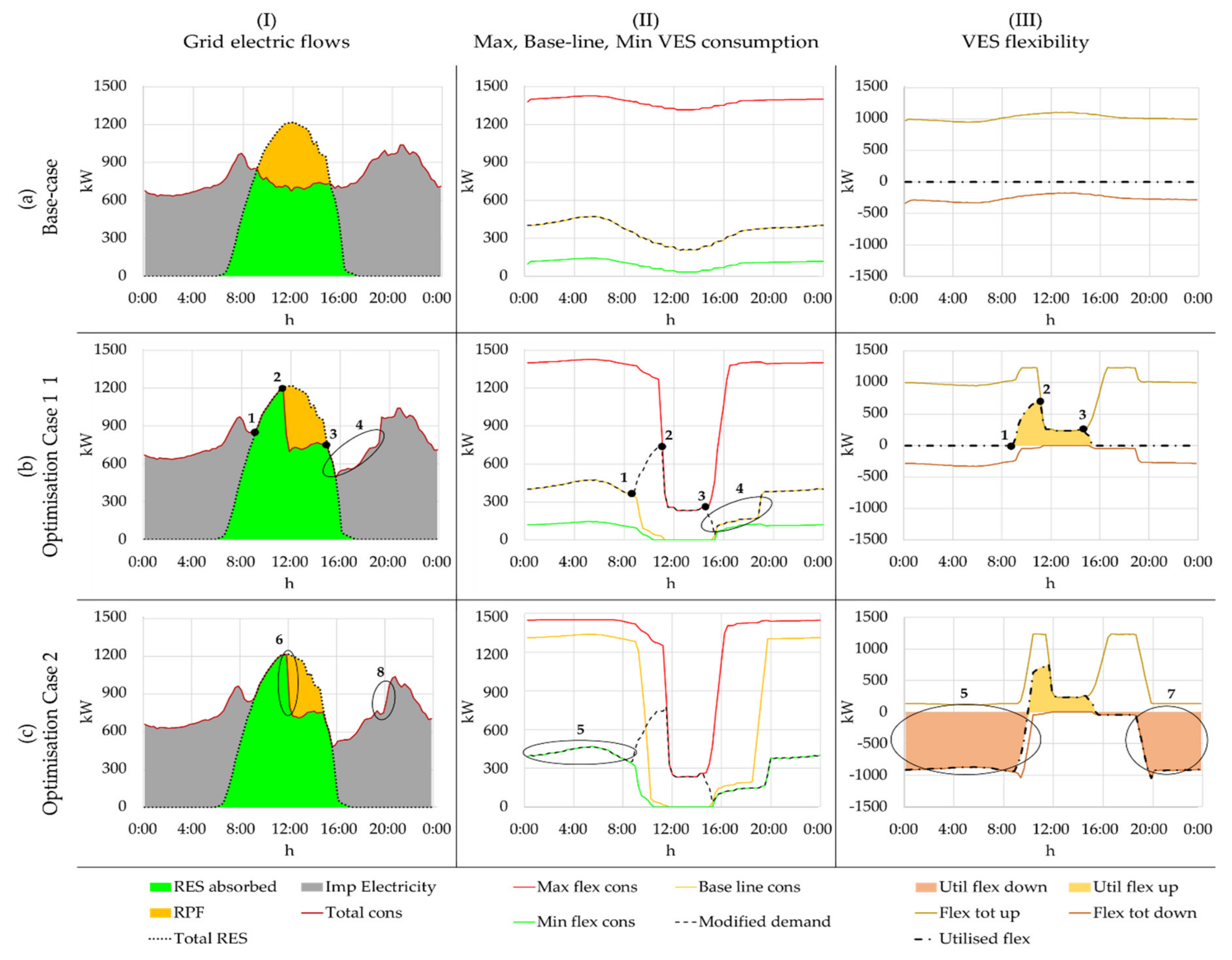
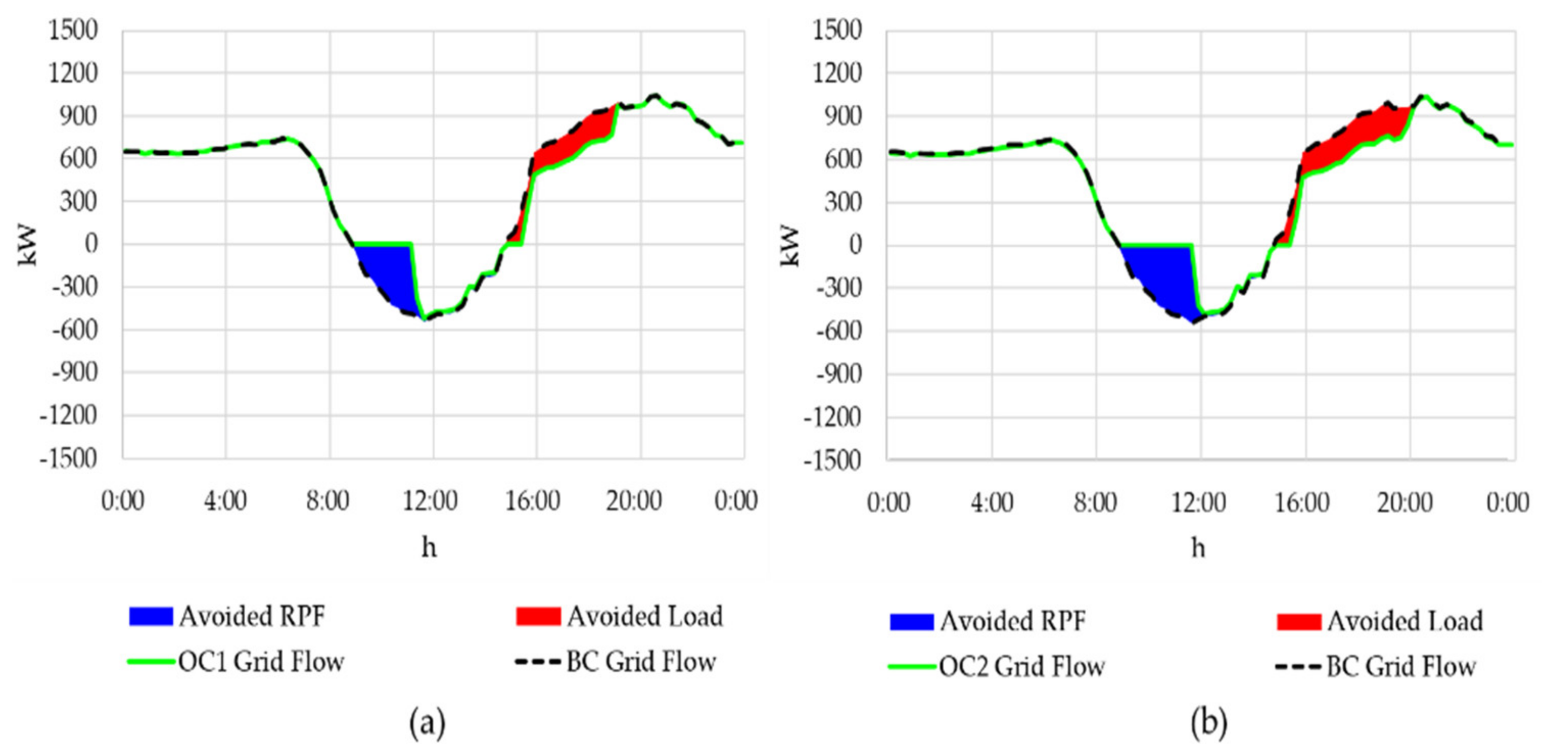
  • Base Case (BC): The VES-enabled flexibility is not exploited and the end-user demand; therefore, remains at its baseline value. The indoor temperature of the buildings is maintained at the baseline value that maximises the thermal comfort of the occupants.
  • Optimisation Case 1 (OC1): The VES-enabled flexibility is estimated and utilised with the objective of maximising the absorption of the local RESs generation. During these periods, the temperature of the building is increased, without violating the upper temperature boundary, which was estimated during the profiling of the occupants’ thermal comfort. During time periods in which there is no RESs over-production, the end-users’ demand follows the baseline trend.
  • Optimisation Case 2 (OC2): The VES-enabled flexibility is utilised to obtain the maximum absorption of local RESs generation through the same approach as that of OC1. However, during the periods of time when there is no RESs production, the buildings adopt a strategy of minimised energy consumption through the control of their LP2H systems at the lower comfort temperature boundary, which is based on the results of the comfort profiling. In this way, the storage capacity of the VES-enabled building is maximised, as it increases the allowed temperature variation while following a building-level energy efficiency strategy.
In all the scenarios, the SCCE receives demand flexibility forecasts from the VES module and dispatches demand modification set-points on the basis of these forecasts. The flexibility forecasts are comfort preserving and therefore ensure that the thermal demand of the end-users is satisfied. At the same time, the demand modification set-points ensure that the RESs overproduction is absorbed as much as possible to reduce the Reverse Power Flow. As detailed in Section 2.2.2, the installed LP2H units provide a certain amount of flexibility, since the thermal demand of the building could be modulated through smart exploitation of the thermal properties of the building envelope.
The results of the scenario were evaluated with respect of the benefits that they provide to the energy district and from the point of view of the occupants, in terms of how much the indoor temperature varies from its optimum value. The calculated Key Performance Indicators (KPIs) are presented hereafter:
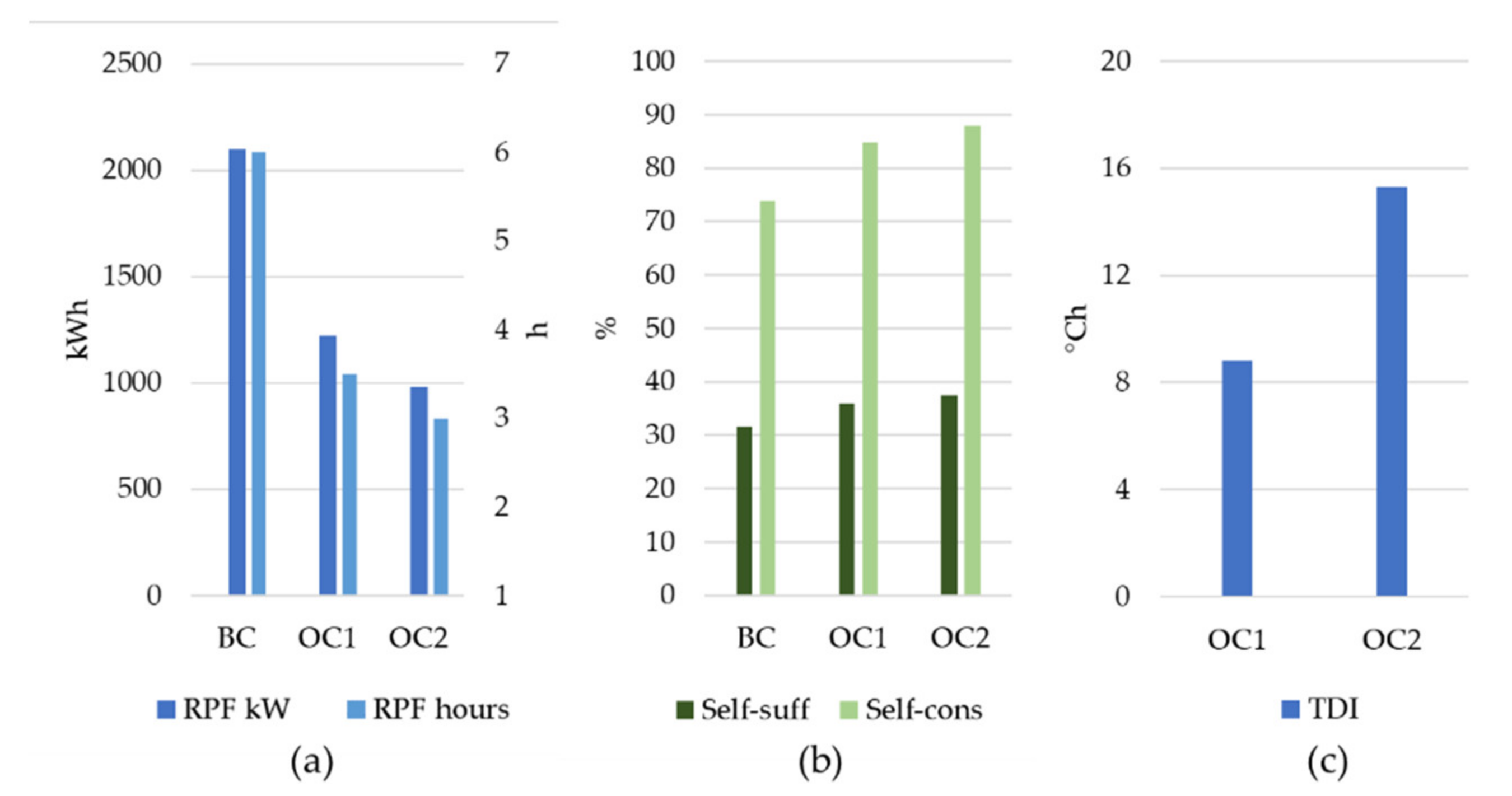
  • Reverse Power Flow (RFP): The RPF is calculated for each scenario as the surplus production (in kWh) of the RESs generation that is not absorbed locally or timely.
    R P F =                                                                                                                                 0 ,     g e n t n c o n t n < 0 n     1 N P g e n t n P c o n t n   t s t e p 3600 ,     g e n t n c o n t n 0
    where P g e n t n is the total generation in the scenario at time step t n and P c o n t n is the total consumption of the investigated part of the grid.
  • Grid Self-Sufficiency (Ss): The grid Self-Sufficiency ( % ) represents the percentage of electricity demand that is covered by the local PV production:
    S s = E t o t ,   R E S R P F E c o n s · 100
    where E t o t ,   R E S is the total PV production and E c o n s is the total electric consumption of the local grid. The higher the Grid Self-Sufficiency is, the less electric energy withdrawn from the transmission grid. Since the distributed generation considered in this scenario was composed of RESs generators, this metric is also representative of RESs penetration.
  • Grid Self-Consumption (Sc): The grid Self-Consumption % represents the percentage of PV electricity production that is consumed locally in the scenario. The higher the value of this KPI is, the lower the amount of RESs overproduction that is transformed to RPF.
    S c = E t o t ,   R E S R P F E t o t ,   R E S · 100
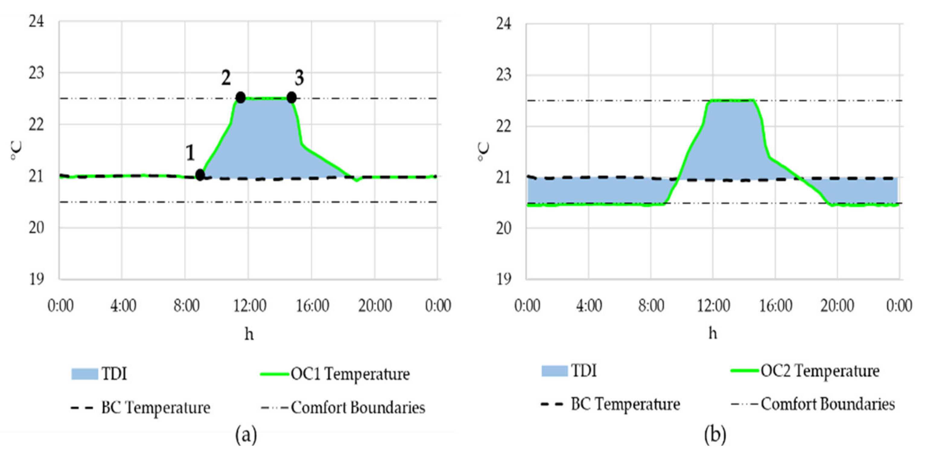
  • Thermal Discomfort Indicator (TDI): PLANET VES-enabled flexibility profiling is comfort preserving, in the sense that it takes into account the upper and lower comfort temperature boundaries as inherent optimisation constraints. These temperature thresholds are inferred from thermal comfort profiling (as described in Section 2.2.2) and represent a compromise status in which the occupant has a higher probability of being in a state of comfort that in discomfort. However, an optimal comfort is achieved when the temperature lies within the narrower range defined as the baseline comfort temperature zone. To this end, the lower “comfort indicator” is calculated for each of the optimisation cases:
    T D I = n 1 N T B C t n T O C t n   t s t e p 3600 ,     T O C t n T B C t n < 0 n 1 N T O C t n T B C t n t s t e p 3600 ,     T O C t n T B C t n 0
    The above KPI refers to a benchmark building and constitutes a metric that includes both the temperature deviation from the Base Case temperature and the time duration of such a deviation. The Thermal Discomfort Indicator (TDI) is expressed in {°C∙h}, and the smaller the value is, the lower the deviation from the preservation of optimal comfort during demand modulation events.

4. Results and Discussion

The analysed Base Case scenario is characterised by surplus electricity, generated during local PV plant peaks, which triggers Reverse Power Flows (see Figure 7(aI)). In the Base Case scenario, the electric heating consumption is maintained at the baseline for all the horizons considered in the simulation, without making use of the demand flexibility enabled by VES (see Figure 7(aII,III)). The electric heating load is lower at mid-day, because of the higher external temperature. In general, the higher the external temperature is, the lower the electrical demand for heating purposes.
In Optimisation Case 1, the RPF is reduced as a result of the optimisation control strategy (see Figure 7(bI)). The sum of the electrical demand of the buildings coincides with that of the baseline consumption up to point 1 in Figure 7(bI,II), until which the local RESs do not exceed the respective consumption. Beyond this point, the grid optimiser modulates the LP2H consumption in order to absorb the surplus renewable energy as much as possible. The overproduction is completely absorbed up to point 2, and at this point the VES-enabled buildings increase their electrical consumption, due to space pre-heating, until the buildings reach the indoor temperature threshold, which coincides with the upper comfort boundary temperature (see Figure 8a) and inhibits a further increase in the electric heating consumption (see Figure 7(bII,III)). The electric heating in the buildings is maintained at the maximum consumption beyond point 2 and up to point 3, as per Figure 7, which is actually the period of time of excess local renewable production, and employs all the available upwards flexibility. As a result, the buildings accumulate thermal energy, which is temporarily “stored”, thanks to the thermal inertia of the building envelope. This pre-heating technique, which is powered by renewable energy sources, leads to a reduced electrical demand during the hours that follow the PV peaks (see point 4 in Figure 7(bI,II)).
Optimisation Case 2 is reported in row c in Figure 7. In this case, the grid control strategy dictates that the flexible electric heating loads should operate at their minimum set-points at times when there is no renewable energy surplus production and that they should exploit all the available downwards flexibility (point 5 in Figure 7(cII,III)). The internal temperature at the building-level is maintained at its lower comfort boundary temperature (see Figure 8b), thus exploiting the potential of the downwards flexibility and at the same time increasing the available temperature gap that has to be covered using the subsequent surplus PV production. The latter can be perceived as an increase in the upwards flexibility of the pending time horizon (see point 6 in Figure 7(cI)). The VES-enabled downwards flexibility is again utilised after the PV overproduction time slot (see point 7 in Figure 7(cIII)) in the building-level energy efficiency frame. This leads to an overall larger reduction in electricity consumption than for OC1 (see point 8 in Figure 7(cI)).
The benefits of the exploitation of the VES-enabled flexibility from the network are evident from a comparison of the electricity flow profiles in the Base Case with those in the Optimised Cases, as shown in Figure 9. The positive part of the graph represents the electric energy withdrawn from the upstream network, while the negative part is the energy flow that is injected into the high voltage network from the medium voltage network (i.e., the RPF). It can be noted that both of the two used control strategies give similar results: Thanks to the exploitation of the VES-enabled and LP2H-powered demand flexibility, it is possible to absorb part of the RPF and, at the same time, to reduce the electricity withdrawn from the transmission network, without affecting the end-users’ thermal comfort to any great extent. The reduction in the RPF occurs because part of the renewable surplus production is absorbed by the VES-enabled buildings in order to cover any heating needs that arise some hours later. The electric consumption is lower for the following hours as a result of the temporary storage of the thermal energy generated from the building envelopes, due to the pre-heating, since less energy is required, in comparison with the BC, to maintain the interiors at acceptable thermal comfort levels (see Figure 9).
The RPF was reduced by around 40%, in comparison to the BC, in terms of both energy and duration in OC1 and more than 50% in OC2 (see Figure 10a). The improvement in the integration of renewable energy is also reflected in an increase of both the self-consumption and the self-sufficiency metrics. The former grows from 74% for the Base Case to 85% for OC1 and 88% for OC2. The latter increases from 32% for the Base Case to 36% for OC1 and 38% OC2 (see Figure 10b).
In essence, the smart exploitation of the thermal demand flexibility converted into electric flexibility by the LP2H systems under a VES framework, allows for a more efficient integration of distributed renewable energy. OC2, which makes use of flexibility exploitation from an energy efficiency point of view, displays even better overall results. However, the more extended the VES-enabled flexibility exploitation is, the higher the impact on the internal temperature conditions of the buildings. Notwithstanding, the VES module ensures that thermal comfort is maintained within acceptable levels for all the cases, thereby protecting the residents from discomfort during the utilisation of the demand flexibility. However, as can be noted from the TDI parameter (see Figure 10c), the periods during which the internal temperatures of the buildings is sub-optimal, in terms of thermal comfort, increase for OC2.

5. Conclusions

The increase in non-dispatchable distributed generation will lead to new paradigms in the management of energy networks. If the generation follows intermittent and variable patterns, the demand shall be able to adjust accordingly to balance the grid and ensure the supply. This will pave the way towards new demand flexibility resources.
A new, high-accuracy Virtual Energy Storage model, which is based on a multi-resistance and multi-capacitance modelling approach (3R2C model), was presented. The developed model allows the electrical response of this technology to be controlled externally while maintaining internal comfort constraints. The model was integrated with a co-simulation structure within the PLANET Decision Support System to simulate multi-energy energy scenarios.
This paper has analysed the Virtual Energy Storage-enabled demand flexibility that couples building-level Power-to-Heat energy conversion systems installed in residential and commercial buildings to transpose the intrinsic flexibility of the thermal demand to the electricity sector. Unlike other large-scale technologies that are capable of providing electrical flexibility, which are characterised by significant investment costs, such as Battery Energy Storage Systems (BESS) or P2G systems, the Virtual Energy Storage system uses the thermal properties of the building element that are already present in any scenario as the energy storage source, without any additional investment costs.
PLANET DSS was used to simulate a scenario with 30% renewable energy penetration. As this system is weather-driven, the renewable distributed generation leads to a considerable generation surplus during certain time slots when the ambient conditions permit such a surplus. As a result, sub-optimal grid flows appear and these lead to Reverse Power Flows, increased system losses, RESs curtailment, etc. In the present study, as part of the control strategies adopted to averse the negative impact of RESs overproduction on the network, the electric heating of the VES-enabled buildings is controlled at an aggregated district-level with two different control algorithms. The control systems ensure that the temperature always remains within an acceptable thermal comfort range. It was shown that a higher exploitation of the LP2H flexibility leads to higher benefits, from an energetic point of view, while, on the other hand, the more the flexibility is used, the more the internal temperature of the buildings is affected, which in turn causes a greater deviation from the optimum comfort temperature. In this study, the benefits and negative aspects are presented in a quantified form in an attempt to evaluate the overall trade-off of the exploitation of demand flexibility for the optimisation of energy flows.
The Reverse Power Flow issue can be alleviated drastically through the exploitation of the VES-enabled flexibility: In the analysed scenario, the Reverse Power Flow was reduced by about 50%, in terms of both energy and duration. The control of the LP2H energy consumption in fact allowed an optimal use of the renewable resources, which is reflected in both the self-consumption and self-sufficiency of the network.

Author Contributions

Methodology, M.B. and A.P.; software, G.F., D.T. and G.G.; validation, D.T. and G.G.; investigation, G.F. and V.K.; writing—original draft preparation, G.F., V.K. and M.B; writing—review and editing, G.F. and V.K.; visualization, G.F. and V.K.; supervision, M.B. and A.P. All authors have read and agreed to the published version of the manuscript.

Funding

This research has received support from the EU Planet project funded as part of the European Union’s Horizon 2020 research and innovation programme under grant agreement No. 773839.

Acknowledgments

The authors would like to thank Andrea Mazza from the Politecnico di Torino (Turin, Italy) for his advice and contribution to the research.

Conflicts of Interest

The authors declare no conflict of interest.

References

  1. Meinshausen, M.; Meinshausen, N.; Hare, W.; Raper, S.C.; Frieler, K.; Knutti, R.; Frame, D.J.; Allen, M.R. Greenhouse-gas emission targets for limiting global warming to 2 C. Nature 2009, 458, 1158–1162. [Google Scholar] [CrossRef] [PubMed]
  2. Seeley, J.T.; Romps, D.M. The Effect of Global Warming on Severe Thunderstorms in the United States. J. Clim. 2015, 28, 2443–2458. [Google Scholar] [CrossRef]
  3. United Nations Climate Change. What Is the Paris Agreement? Available online: https://unfccc.int/process-and-meetings/the-paris-agreement/what-is-the-paris-agreement (accessed on 8 July 2020).
  4. European Commission. Clean Energy for All Europeans; Publications Office of the European Union: Luxembourg, Luxembourg, 2019. [Google Scholar]
  5. Lehtveer, M.; Mattsson, N.; Hedenus, F. Using resource based slicing to capture the intermittency of variable renewables in energy system models. Energy Strat. Rev. 2017, 18, 73–84. [Google Scholar] [CrossRef]
  6. Jacobson, M.Z.; Delucchi, M.A.; Bauer, Z.A.; Goodman, S.C.; Chapman, W.E.; Cameron, M.A.; Bozonnat, C.; Chobadi, L.; Clonts, H.A.; Enevoldsen, P.; et al. 100% Clean and Renewable Wind, Water, and Sunlight All-Sector Energy Roadmaps for 139 Countries of the World. Joule 2017, 1, 108–121. [Google Scholar] [CrossRef] [Green Version]
  7. Andrychowicz, M. Comparison of the Use of Energy Storages and Energy Curtailment as an Addition to the Allocation of Renewable Energy in the Distribution System in Order to Minimize Development Costs. Energies 2020, 13, 3746. [Google Scholar] [CrossRef]
  8. Chicco, G.; Riaz, S.; Mazza, A.; Mancarella, P. Flexibility from Distributed Multienergy Systems. Proc. IEEE. 2020, 108, 1496–1517. [Google Scholar] [CrossRef]
  9. Ciocia, A.; Boicea, V.A.; Chicco, G.; Di Leo, P.; Mazza, A.; Pons, E.; Spertino, F.; Hadj-Said, N. Voltage control in low-voltage grids using distributed photovoltaic converters and centralized devices. IEEE Trans. Ind. Appl. 2018, 55, 225–237. [Google Scholar] [CrossRef]
  10. Diaz-Londono, C.; Colangelo, L.; Ruiz, F.; Patino, D.; Novara, C.; Chicco, G. Optimal Strategy to Exploit the Flexibility of an Electric Vehicle Charging Station. Energies 2019, 12, 3834. [Google Scholar] [CrossRef] [Green Version]
  11. De Luca, G.; Ballarini, I.; Lorenzati, A.; Corrado, V. Renovation of a social house into a NZEB: Use of renewable energy sources and economic implications. Renew. Energy 2020, 159, 356–370. [Google Scholar] [CrossRef]
  12. Badami, M.; Fambri, G. Optimising energy flows and synergies between energy networks. Energy 2019, 173, 400–412. [Google Scholar] [CrossRef]
  13. Jin, X.; Wang, X.; Mu, Y.; Jia, H.; Xu, X.; Qi, Y.; Yu, X.; Qi, F. Optimal scheduling approach for a combined cooling, heating and power building microgrid considering virtual storage system. In Proceedings of the 2016 IEEE Power and Energy Society General Meeting (PESGM), Tianjin, China, 17 July 2016. [Google Scholar]
  14. Sikder, O.; Jansson, P.M. Thermal inertia of a building as virtual energy storage: A sustainable solution for smart grids. In Proceedings of the 2018 53rd International Universities Power Engineering Conference (UPEC), Glasgow, Scotland, 4–6 September 2018. [Google Scholar]
  15. Asare, P.; Ononuju, C.; Jansson, P.M. Preliminary quantitative evaluation of residential virtual energy storage using power sensing. In Proceedings of the 2017 IEEE Sensors Applications Symposium (SAS), Glassboro, NJ, USA, 13–15 March 2017. [Google Scholar]
  16. PLANET. Planning and Operational Tools for Optimising Energy Flows & Synergies Between Energy Networks. Available online: https://www.h2020-planet.eu/ (accessed on 8 July 2020).
  17. Katsiki, V.; Papanikolaou, A.; Sideris, D.; Makris, S.T.; Nikolopoulos, D.; Petridis, K.; Schröder, A.; Breuers, M.; Mirtaheri, H.; Bortoletto, A.; et al. Deliverable D1.5 PLANET System Architecture Definition, PLANET. 2019. Available online: https://www.h2020-planet.eu/deliverables (accessed on 1 August 2020).
  18. Papanikolaou, A.; Katsiki, V.; Sideris, D.; Mazza, A.; Estebsari, A.; Mirtaheri, H.; Damousis, Y.; Kakardakos, N.; Faropoulos, J.; Skiadaresis, G. Deliverable D1.4 PLANET System Architecture Definition, PLANET. 2019. Available online: https://static1.squarespace.com/static/5a3297ded7bdce9ea2f39f1a/t/5ddd2a00c833493f056f2a08/1574775315046/D1.4_Planet_Final_PU.pdf (accessed on 8 July 2019).
  19. Badami, M.; Fambri, G.; Mancò, S.; Martino, M.; Damousis, I.G.; Agtzidis, D.; Tzovaras, D. A Decision Support System Tool to Manage the Flexibility in Renewable Energy-Based Power Systems. Energies 2019, 13, 153. [Google Scholar] [CrossRef] [Green Version]
  20. Bottaccioli, L.; Patti, E.; Macii, E.; Acquaviva, A. Distributed Infrastructure for Multi-Energy-Systems Modelling and Co-simulation in Urban Districts. In Proceedings of the 7th International Conference on Smart Cities and Green ICT Systems (SMARTGREENS), Funchal, Portugal, 16–18 March 2018. [Google Scholar]
  21. eMEGAsim, Power System and Power Electronic Real-Time Simulator, OPAL-RT. Available online: http://www.opal-rt.com/new-product/emegasim-power-system-and-power-electronic-real-time-simulator (accessed on 11 June 2020).
  22. Bottaccioli, L.; Estebsari, A.; Patti, E.; Pons, E.; Acquaviva, A. Planning and real-time management of smart grids with high PV penetration in Italy. Proc. Inst. Civ. Eng. Eng. Sustain. 2018, 172, 272–282. [Google Scholar] [CrossRef]
  23. Bian, D.; Kuzlu, M.; Pipattanasomporn, M.; Rahman, S.; Wu, Y. Real-time co-simulation platform using OPAL-RT and OPNET for analyzing smart grid performance. In In Proceedings of the 2015 IEEE Power & Energy Society General Meeting, Denver, CO, USA, 26–30 July 2015. [Google Scholar]
  24. Mirtaheri, H.; Bortoletto, A.; Fantino, M.; Bertone, F.; Li, Y.; Damousis, Y.; Agtzidis, D.; Katsiki, V.; Papanikolaou, A.; Schröder, A.; et al. Deliverable D3.5 District-Level Storage and Conversion Management & Coordination Engine (SCCE). PLANET 2019, in press. [Google Scholar]
  25. Barooah, P. Virtual energy storage from flexible loads: Distributed control with QoS constraints. In Smart Grid Control; Stoustrup, J., Anuradha Annaswamy, A., Chakrabortty, A., Qu, Z., Eds.; Springer: Cham, Switzerland, 2019; pp. 99–115. [Google Scholar]
  26. Eurelectric; EY. Report on the Future Role of DSOs in Europe. Getting Ready: DSO 2.0. 2019. Available online: https://www.eurelectric.org/media/3637/ey-report-future-of-dsos.pdf (accessed on 8 July 2020).
  27. Klaassen, E.; Van der Laan, M. Energy and Flexibility Services for Citizens Energy Communities. U.S.E. Framework. 2019. Available online: https://www.buildup.eu/sites/default/files/content/usef-white-paper-energy-and-flexibility-services-for-citizens-energy-communities-final-cm.pdf (accessed on 8 July 2020).
  28. Makris, S.; Nikolopoulos, D.; Ververidis, C.; Katsiki, V.; Badami, M.; Fambri, G.; Granroth-Wilding, H.; Hussam, S.; Soppela, O.; Kakardakos, N.; et al. Deliverable D3.3 PLANET P2H-Enabled Human-Centric VES Module, PLANET. 2019. Available online: https://static1.squarespace.com/static/5a3297ded7bdce9ea2f39f1a/t/5ddd2ab2880bee4473692781/1574775481127/D3.3_Planet_Final_PU.pdf (accessed on 8 July 2019).
  29. Malavazos, C.; Tsatsakis, K.; Tsitsanis, A. Towards a “context aware” flexibility profiling mechanism for the energy management environment. In Proceedings of the MedPower Conference, Athens, Greece, 2–5 November 2014. [Google Scholar]
  30. Seungjae, L.; Bilionis, I.; Karava, P.; Tzempelikos, A. A Bayesian Approach for Learning and Predicting Personal Thermal Preference. In Proceedings of 4th International High-Performance Buildings Conference, West Lafayette, IN, USA, 11–14 July 2016. [Google Scholar]
  31. Enescu, D. A review of thermal comfort models and indicators for indoor environments. Renew. Sustain. Energy Rev. 2017, 79, 1353–1379. [Google Scholar] [CrossRef]
  32. Papanikolaou, A.; Nassos, T.; Alexandros, D.; Dionisis, N.; Katsiki, V.; Fantino, M.; Kakardakos, N.; Faropoulos, j.; Skiadaresis, G.; Vourkas, H.; et al. Deliverable D2.3 Human-Centric, Context-Aware VES Demand Flexibility Profiles, PLANET. 2019. Available online: https://www.h2020-planet.eu/s/D23_Planet_Final_PU.pdf (accessed on 8 July 2019).
  33. Dall’O, G. Green Energy Audit of Buildings: A Guide for a Sustainable Energy Audit of Buildings; Springer: London, UK, 2013. [Google Scholar]
  34. Bacher, P.; Madsen, H. Identifying suitable models for the heat dynamics of buildings. Energy Build. 2011, 43, 1511–1522. [Google Scholar] [CrossRef] [Green Version]
  35. Katsiki, V.; Ververidis, C.; Petridis, K.; Bompard, E.; Chicco, G.; Chomaz, R.; Agtzidis, D.; Damousis, Y.; Tsotakis, C.; Afentoulis, K.; et al. Deliverable D5.3; Simulation Lab Set-up and VES Model Calibration Report, PLANET. 2020. in press. Available online: https://www.h2020-planet.eu/deliverables (accessed on 8 July 2019).
  36. Camacho, E.F.; Alba, C.B. Model Predictive Control; Springer Science & Business Media: Berlin/Heidelberg, Germany, 2013. [Google Scholar]
  37. Genest, O.; Pons, L.; Valckenaers, P.; Crihan, F. Main Findings and Recommendations: Data Management Working Group; BRIDGE Horizon 2020. 2019. Available online: https://www.h2020-bridge.eu/wp-content/uploads/2018/06/BRIDGE-Data-Management-WG-Findings-and-Reco-July-2019.pdf (accessed on 8 July 2019).
  38. Damousis, Y.; Agtzidis, D.; Badami, M.; Fambri, G.; Diaz-Londono, C. Deliverable D4.2 PLANET Communication Middleware Development & Configuration; PLANET. 2019. Available online: https://static1.squarespace.com/static/5a3297ded7bdce9ea2f39f1a/t/5ddd2b96516b877c21373f38/1574775708936/D4.2_Planet_Final_PU.pdf (accessed on 8 July 2019).
  39. Carpaneto, E.; Chicco, G. Probability distributions of the aggregated residential load. In Proceedings of the 9th International Conference on Probabilistic Methods Applied to Power Systems, Stockholm, Sweden, 11–15 June 2006. [Google Scholar]
  40. SOREA. Available online: https://www.sorea-maurienne.fr/ (accessed on 20 March 2020).
  41. Renewables.ninja. Available online: https://www.renewables.ninja/ (accessed on 20 March 2020).
Figure 1. PLANET (PLAnning and operational tools for optimising energy flows and synergies between energy NETworks) storage/conversion technologies and the corresponding asset coupling points.
Energies 13 05128 g001
Figure 2. Conceptual architecture of the PLANET Decision Support System (DSS).
Energies 13 05128 g002
Figure 3. Decomposition of the Virtual Energy Storage (VES) module.
Energies 13 05128 g003
Figure 4. Sequence of interactions between VES within the PLANET tool.
Energies 13 05128 g004
Figure 5. Analysed scenario.
Energies 13 05128 g005
Figure 6. (a) Residential/commercial consumption (p.u.). (b) PV production (p.u.) and ambient temperature (°C).
Energies 13 05128 g006
Figure 7. Resulting energy flows, consumption and flexibility curves for all three (3) scenarios.
Energies 13 05128 g007
Figure 8. Mean internal temperature of the VES buildings. Comparison of Base Case (BC) and Optimisation Case 1 (OC1) (a), comparison of BC and Optimisation Case 2 (OC2) (b).
Energies 13 05128 g008
Figure 9. Power flow in the electrical network. Comparison of BC and OC1 (a), comparison of BC and OC2 (b).
Energies 13 05128 g009
Figure 10. Reverse power flow (a); self-sufficiency and self-consumption (b); thermal discomfort indicator (c).
Energies 13 05128 g010
Table 1. Overview of the flexibility optimisation algorithm.
min / max control   Consumption   over   the   forecasted   horizon
Subject   to   constraints   Thermal   comfort   boundaries     Space   thermal   model LP2H   energy   conversion   specifications
Table 2. Input, Output and Configuration Parameters of the PLANET VES module.
VariablesNameUnitsType
Configuration Parameters
R1, R2, R3Conduction, convection and infiltration-related resistances°C/WFloat
C1, C2Thermal capacitancesJ/°CFloat
p1, p2Distribution coefficients of the solar gains-Float
p3, p4Distribution coefficients of the electrical heating load-Float
T c o m f u p , T c o m f d o w n Thermal comfort boundaries°CFloat
n r e s Number of residential buildings in the VES Portfolio-Integer
n c o m Number of commercial buildings in the VES Portfolio-Integer
Input Parameters
t n Time point secFloat
T e x t Outdoor temperature forecast°CFloat
QsolarGlobal horizontal irradianceW/m2Float
T i n Initial indoor temperature°CFloat
PconsDemand modification (request to apply consumption)WFloat
Output Parameters
P f l e x , u p Upwards flexibilityWFloat
P f l e x ,   d o w n Downwards flexibilityWFloat
P b a s e Baseline consumptionWFloat
Table 3. Composition of the analysed scenario.
Network NodePV Nominal Power
kW
VES Buildings
(Residential and Commercial Users)
Flexible Load
Aggregated LP2H
kW
Fixed Load
kW
Node 1-Res: 100. Com: 10520830
Node 2300Res: 60. Com: 5310495
Node 3-Res: 80. Com: 20440700
Node 4350Res: 50. Com: 15280445
Node 5-Res: 90. Com: -450720
Node 6400Res: 60. Com: 5310495
Node 7300Res: 70. Com: 15380605
Node 8350Res: 40. Com: -200320
Total1700Res: 550. Com: 7028904610

