The Numerical Simulation Study of the Oil–Water Seepage Behavior Dependent on the Polymer Concentration in Polymer Flooding

Abstract

It is well acknowledged that due to the polymer component, the oil–water relative permeability curve in polymer flooding is different from the curve in waterflooding. As the viscoelastic properties and the trapping number are presented for modifying the oil–water relative permeability curve, the integration of these two factors for the convenience of simulation processes has become a key issue. In this paper, an interpolation factor $\Omega$ that depends on the normalized polymer concentration is firstly proposed for simplification. Then, the numerical calculations in the self-developed simulator are performed to discuss the effects of the interpolation factor on the well performances and the applications in field history matching. The results indicate that compared with the results of the commercial simulator, the simulation with the interpolation factor $\Omega$ could more accurately describe the effect of the injected polymer solution in controlling water production, and more efficiently simplify the combination of factors on relative permeability curves in polymer flooding. Additionally, for polymer flooding history matching, the interpolation factor $\Omega$ is set as an adjustment parameter based on core flooding results to dynamically consider the change of the relative permeability curves, and has been successfully applied in the water cut matching of the two wells in Y oilfield. This investigation provides an efficient method to evaluate the seepage behavior variation of polymer flooding.

1. Introduction

After the primary depletion and the waterflooding developmental processes, there is still much oil remaining in reservoirs [1,2,3]. Since the water cut of oil blocks gains over 90%, resulting in no longer remarkable waterflooding economic benefits, polymer flooding has been widely applied in oilfields as one of the main enhanced oil recovery (EOR) methods [4,5,6]. In order to clearly characterize the oil–water flow capacity in the polymer flooding, the oil and water relative permeabilities are the focus of this study.

In past decades, numerous researchers have reported that for polymer flooding, the oil–water relative permeability curve is regarded as an important role in describing seepage behavior, well performance matching and developmental plans establishment. To reflect the effect of polymer solutions on relative permeability curves, various numerical methods have been employed based on experiments or field data. In 1989, pore-network modeling (PNM) for describing the polymer shear in capillaries was presented [7]. Based on this research, dynamic PNM and adaptive dynamic PNM were respectively applied to consider the complicated influence factors of the relative permeabilities in polymer flooding, such as polymer properties [8], interfacial tension and capillary number [9], rock wettability, and the hysteresis phenomenon [10,11]. Although the PNM has the ability to intensively describe the interaction between solid surface and polymer solution, the scale of the PNM model could hardly achieve the representative elementary volume (REV) of the actual field. For the field-scale application, automatic-history-matching methods have been used to inversely calculate the oil–water relative permeability of polymer flooding [12]. With more robust inversion methods based on the iterative ensemble Kalman filter (EnKF) [13] or the Levenberg–Marquardt (LM) algorithm [14], relative permeabilities and rock properties were modified by large actual data and massive simulation computation [15,16]. To further improve the predictive capability of numerical evaluation, the simulator UTCHEM combined the Corey-type relative permeability model with the dimensionless trapping number [17,18], which depends on the interface tension (IFT), rock permeability, buoyancy force and viscous force [19,20,21]. The residual saturation in the relative permeability models also could be dynamically recalculated by the trapping number in the process of polymer injection [22]. Besides the trapping number, the viscoelastic properties of polymers were paid attention to improve the microscopic oil displacement efficiency [23,24]. In the presented polymer flooding simulator, the viscoelastic properties, which depend on the polymer concentration and the relative molecular mass of polymers [25], were combined with the trapping number to describe the oil saturation variation and the increase of the oil’s relative permeability [26]. To avoid the fluid modeling failure caused by the missing date of polymer properties and to improve the computational efficiency, the oil–water relative permeability curves for polymer flooding in the commercial simulator were modified by polymer absorption without considering the factors, viscoelastic properties or trapping number [27].

In summary, many calculated methods have been emphasized to describe the oil–water relative permeabilities in polymer solutions. Caused by the viscoelastic properties and trapping number, the variation of the fluid flow capability has been fully and carefully considered in non-commercial scientific simulators; however, few researchers have explored the synthesis and simplification of the two main factors for their convenient application in simulation processes, such as history matching adjustment.

To fill this gap, a polymer concentration interpolation factor $\Omega$ is presented to simplify the two main factors and conveniently reflect the flow behavior in polymer solutions. Then, compared with the results of the commercial simulator, the case study is launched to discuss the effect of the factor $\Omega$ on well performances. Finally, with the experimental results, the factor $\Omega$ is set as a flexible parameter to successfully match the polymer flooding water cut of two producers in Y oilfield.

2. Methodology

2.1. Assumption

To construct the numerical calculation of the polymer flooding, some assumptions are made in this work: (1) The oil phase, water phase and the polymers are considered as three components; (2) The percolation of each component in the formation is isothermal and obeys the Darcy flow model; (3) The solubility of the polymer in the oil phase is neglected; (4) The oil–water flow capability could be affected by the polymer concentration.

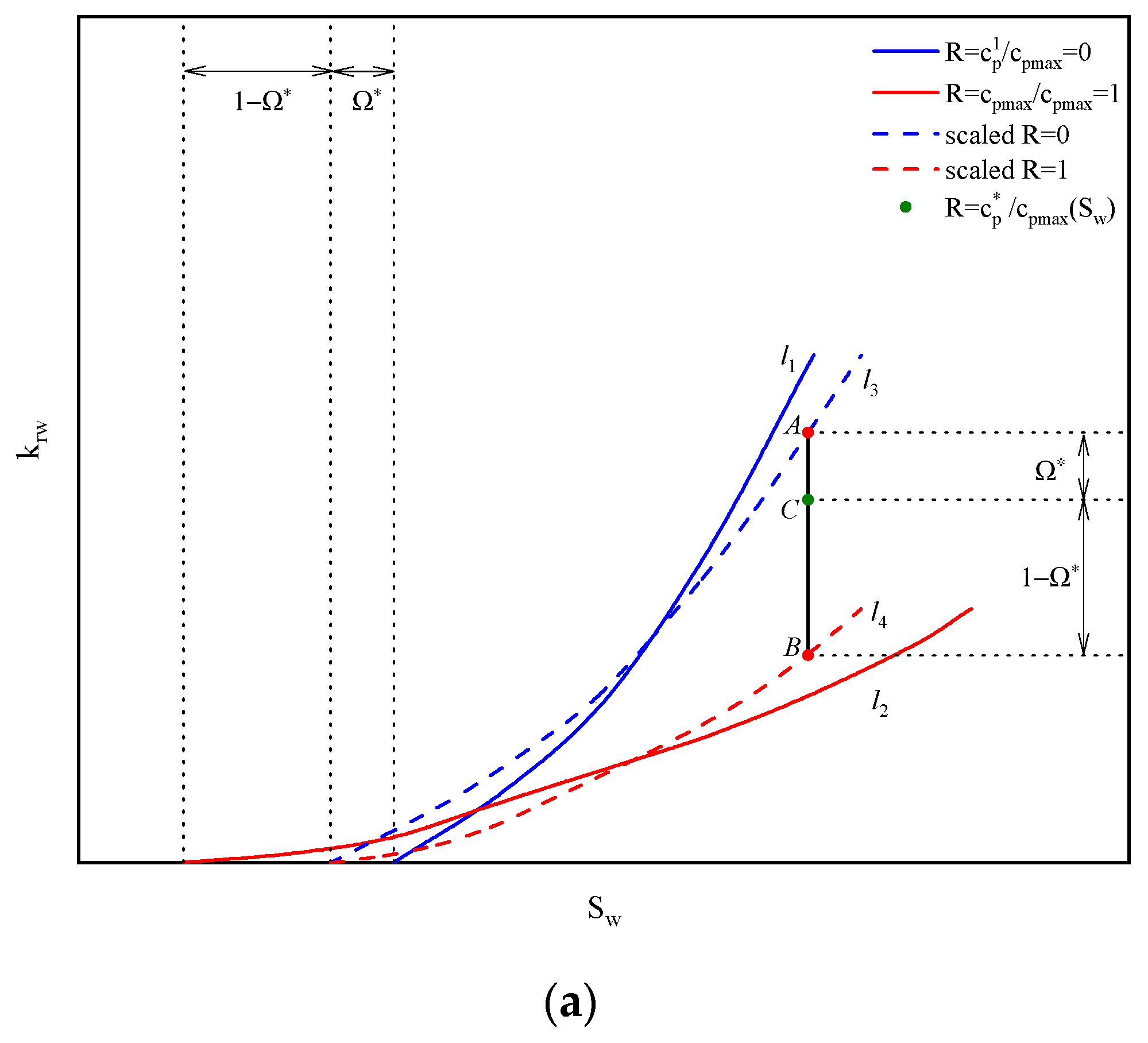
2.2. Polymer Concentration Interpolation Model of Oil–Water Relative Permeabilities

To integrate the effect of the viscoelastic properties and the trapping number into oil–water relative permeabilities, the polymer concentration interpolation model is presented in this work. In the interpolation model, polymer concentration is selected to concisely reflect the viscoelastic properties and the interface tension (IFT) based on the relative permeability curves of polymer flooding experiments [28,29,30], since the relative permeability curves are for a given polymer type. Further, with large intervals of the experimental relative permeabilities between different polymer concentrations, the interpolation method of the relative permeability curves is consulted to dynamically evaluate oil and water mobility based on the change in the polymer concentration.

Based on the above analysis, a table interpolation factor $\Omega$ related to the normalized polymer concentration R is proposed to describe the changing degree of the relative permeability curves (see

Table 1. The interpolation factors.

Normalized Polymer Concentration (R)	${\Omega }$
$c_p^1/c_{p\max }$	0
$c_p^{*}/c_{p\max }$	0.24
...	...
$c_p^2/c_{p\max }$	1

). The normalized polymer concentration is defined as the ratio of the polymer concentration to the maximum polymer concentration ${\mathsf{c}}_{\mathsf{p}\max }$. In Table 1, the ${\mathsf{c}}_{\mathsf{p}}^1$ and ${\mathsf{c}}_{\mathsf{p}}^2$ are the polymer concentrations in the experiments. In the first row of Table 1, R is set as 0 and $\Omega =0$, since this row corresponds to the relative permeability curve at the zero polymer concentration (waterflooding case). In the last row of Table 1, R is 1 constantly and $\Omega =1$, since this row corresponds to the relative permeability curve at the maximum polymer concentration. With the interpolation factor $\Omega$, a new relative permeability curve at the objective normalized polymer concentration can be obtained through the following steps:

Step 1: According to the table function, the specific interpolation factor ${\Omega }^{*}$ of the objective normalized polymer concentration ($R={\mathsf{c}}_{\mathsf{p}}^{*}/{\mathsf{c}}_{\mathsf{p}\max }$) can be calculated. Then, based on the ${\Omega }^{*}$ and taking the equal proportional points from $l_1$ (water-phase relative permeability curve at zero polymer concentration) and $l_2$ (water-phase relative permeability curve at the maximum polymer concentration), the corresponding scaled permeability curves $l_3$ and $l_4$ can be obtained (Figure 1a).

Step 2: Selecting a certain water saturation $S_w$, one can get points A and B on the scaled permeability curves $l_3$ and $l_4$ (Figure 1a).

Step 3: Based on the points A and B, point C can be calculated by a similar method to Step 1.

Step 4: By selecting multiple water saturation values and repeating Step 2 and Step 3, an interpolated water relative permeability at the objective polymer concentration can be calculated.

Further, oil-relative permeability curves can be achieved via the above interpolation method.

Figure 1b is a schematic diagram showing the use of the interpolation method proposed in this paper to calculate the relative permeability curves at any normalized polymer concentration. The blue line and the red line are regarded as the basis relative permeability curves reflecting, respectively, the cases of waterflooding and the maximum polymer concentration. Based on the basis curves, the interpolated relative permeability curves for different polymer concentrations are shown as the dot lines in Figure 1b.

2.3. Mathematical Model

The mathematical model contains the polymer component, the oil phase and the water phase. The key difference from the black oil model is the polymer’s properties. In this paper, the polymer flow mechanisms are considered as follows:

(1)

Polymer adsorption effect

The interactions between the injected polymer solution and the porous media give rise to the mildly viscous adsorption film on the rock surface [31]. Usually, the adsorption effect reduces water permeability by dividing by the actual resistance factor $R_k$ (see Equation (1)). $RRF$ ($RRF\ge 1$) is a constant parameter called the residual resistance factor, which depends on the rock type. $\widehat{c_{p\max }}$ is the maximum adsorbed concentration. The adsorbed concentration $\widehat{c_p}$ is expressed by the generalized Langmuir function of the polymer concentration $c_p$ (see Equation (2)).

$$R_k=1.0+\left(RRF-1.0\right)\cdot \frac{\widehat{c_p}}{\widehat{c_{p\max }}}$$

(1)

$$\widehat{c_p}=\frac{a\cdot {\left(c_p\right)}^m}{1+b\cdot c_p}$$

(2)

(2)

Polymer viscosity effect

The polymer increases the viscosity of the aqueous solutions to improve the oil–water mobility ratio, which is an important factor for enhancing oil recovery. Due to the dissolving degree of polymers, a mixing parameter $\omega$ is defined to calculate the water effective viscosity ${\mu }_{w,eff}$ and the polymer effective viscosity ${\mu }_{p,eff}$, respectively. Based on the Todd–Longstaff mixing model [32], ${\mu }_{p,eff}$ is evaluated in Equation (3), where ${\mu }_p^f\left(c_p\right)$ is the viscosity of the full-mixed solution with the $c_p$ polymer concentration and ${\mu }_{mp}^f\left(c_{p\max }\right)$ describes the viscosity of the $c_{p\max }$ maximum polymer concentration solution. Equation (4) introduces the ${\mu }_{w,eff}$ calculation method, where ${\mu }_{w,e}$ is the water viscosity of the partially dissolved polymer solution. With the same mixing model, ${\mu }_{w,e}$ can be calculated in Equation (5). ${\mu }_w$ is the water-phase viscosity.

$${\mu }_{p,eff}={\mu }_p^f{\left(c_p\right)}^{\omega }\cdot {\mu }_{mp}^f{\left(c_{p\max }\right)}^{1-\omega }$$

(3)

$${\mu }_{w,eff}=1/\left(\frac{1-c_p/c_{p\max }}{{\mu }_{w,e}}+\frac{c_p/c_{p\max }}{{\mu }_{p,eff}}\right)$$

(4)

$${\mu }_{w,e}={\mu }_p^f{\left(c_p\right)}^{\omega }\cdot {\left({\mu }_w\right)}^{1-\omega }$$

(5)

(3)

Polymer rheology effect

Due to the rheology characteristics of non-Newtonian fluids, the viscosity of the polymer solution depends not only on the pressure but also on the shear rate, which differs from the black-oil model. For describing the rheology effect, a shear factor ${\Gamma }_{sh}$ is added in mathematical models to modify ${\mu }_{w,eff}$ and ${\mu }_{p,eff}$ (see Equation (6)). With the same mechanism model as commercial simulators [27], the shear factor ${\Gamma }_{sh}$ is calculated in Equation (7), where $f_{\mu ,w}$ is a table interpolation function to express the effect of the water’s velocity on the sheared water viscosity.

$$\begin{array}{l}{\mu }_{w,eff}^{sh}=\frac{{\mu }_{w,eff}}{{\Gamma }_{sh}}\\ {\mu }_{p,eff}^{sh}=\frac{{\mu }_{p,eff}}{{\Gamma }_{sh}}\end{array}$$

(6)

$${\Gamma }_{sh}=\frac{1+\left({\mu }_p^f\left(c_p\right)/{\mu }_w-1\right)\cdot f_{\mu ,w}}{{\mu }_p^f\left(c_p\right)/{\mu }_w}$$

(7)

(4)

Inaccessible pore volume fraction

As the injected polymers in the solution have large sizes, these polymers cannot access some certain smaller pore throats. In a porous media, the volume of the polymers that have not established effective sweeping percolation is called the inaccessible pore volume (IPV) [33]. To describe the flow characteristics of the polymer solutions, $S_{ipv}$ is defined as a fraction of pore volume, which depends on the rock type and polymer properties.

Based on the functions describing the polymer properties, the flow equations are obtained as follows.

For polymer component:

$$\frac{\partial }{\partial t}\left[\frac{\varphi S_w\left(1-S_{ipv}\right)c_p}{B_w}+{\rho }_r\left(1-S_{ipv}\right)\left(1-\varphi \right)\widehat{c_p}\right]=\nabla \left[\frac{k\cdot k_{rw}\left(c_p\right)\cdot c_p}{B_w\cdot {\mu }_{p,eff}^{sh}\cdot R_k\left(c_p\right)}\nabla \left(p_w-{\rho }_{w}gD\right)\right]+q_{wv}\cdot c_p$$

(8)

For water component:

$$\frac{\partial }{\partial t}\left(\frac{\varphi S_w}{B_w}\right)=\nabla \left[\frac{k\cdot k_{rw}\left(c_p\right)}{B_w\cdot {\mu }_{w,eff}^{sh}\cdot R_k\left(c_p\right)}\nabla \left(p_w-{\rho }_{w}gD\right)\right]+q_{wv}$$

(9)

For oil component:

$$\frac{\partial }{\partial t}\left(\frac{\varphi S_o}{B_o}\right)=\nabla \left[\frac{k\cdot k_{ro}\left(c_p\right)}{B_o{\mu }_o}\nabla \left(p_o-{\rho }_{o}gD\right)\right]+q_{ov}$$

(10)

Saturation equation:

$$S_w+S_o=1$$

(11)

Capillary pressure equation:

$$p_{cow}=p_o-p_w$$

(12)

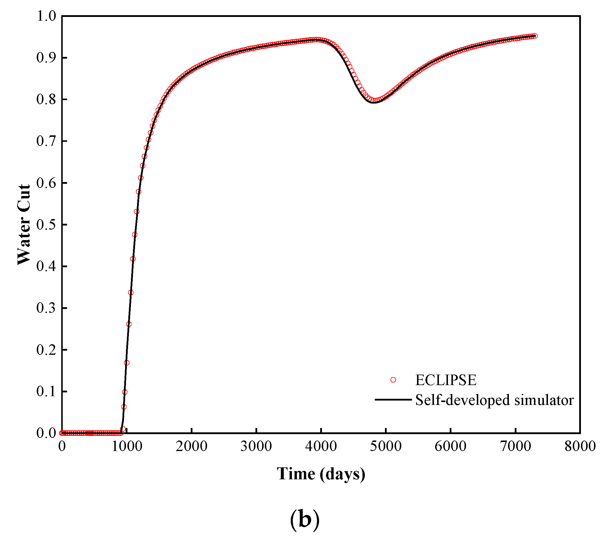
3. Solution and Verification

Figure 2 shows the overall solution workflow of the mathematical model with the polymer concentration interpolation model section. The solution in this work is based on the solution of the black-oil model. After the discretization of the partial differential equations, the pressure, saturation and polymer concentration for each grid are solved by the fully-implicit finite difference method. In each iteration step, the interpolation factor $\Omega$ is determined by the ratio of the polymer concentration to the maximum polymer concentration. Then, the oil–water relative permeability of the corresponding polymer concentration can be interpolated by $\Omega$.

The simulator containing the polymer concentration interpolation model is programmed by Fortran. As the output documents are in the same format as the commercial software, the simulated results could be exhibited with the aid of other software. Figure 3 shows the compared results of the oil recovery and the water cut between our self-developed polymer flooding simulator and the commercial simulator, to demonstrate its reliability [34].

The results of the interpolated relative permeability curves are validated by comparison with the experimental results. In Figure 4, it can be seen that the evaluated relative permeability curves are matched well with the experiment data, which demonstrates the applicability and stability of the interpolation process for polymer concentration variation.

4. Results and Discussion

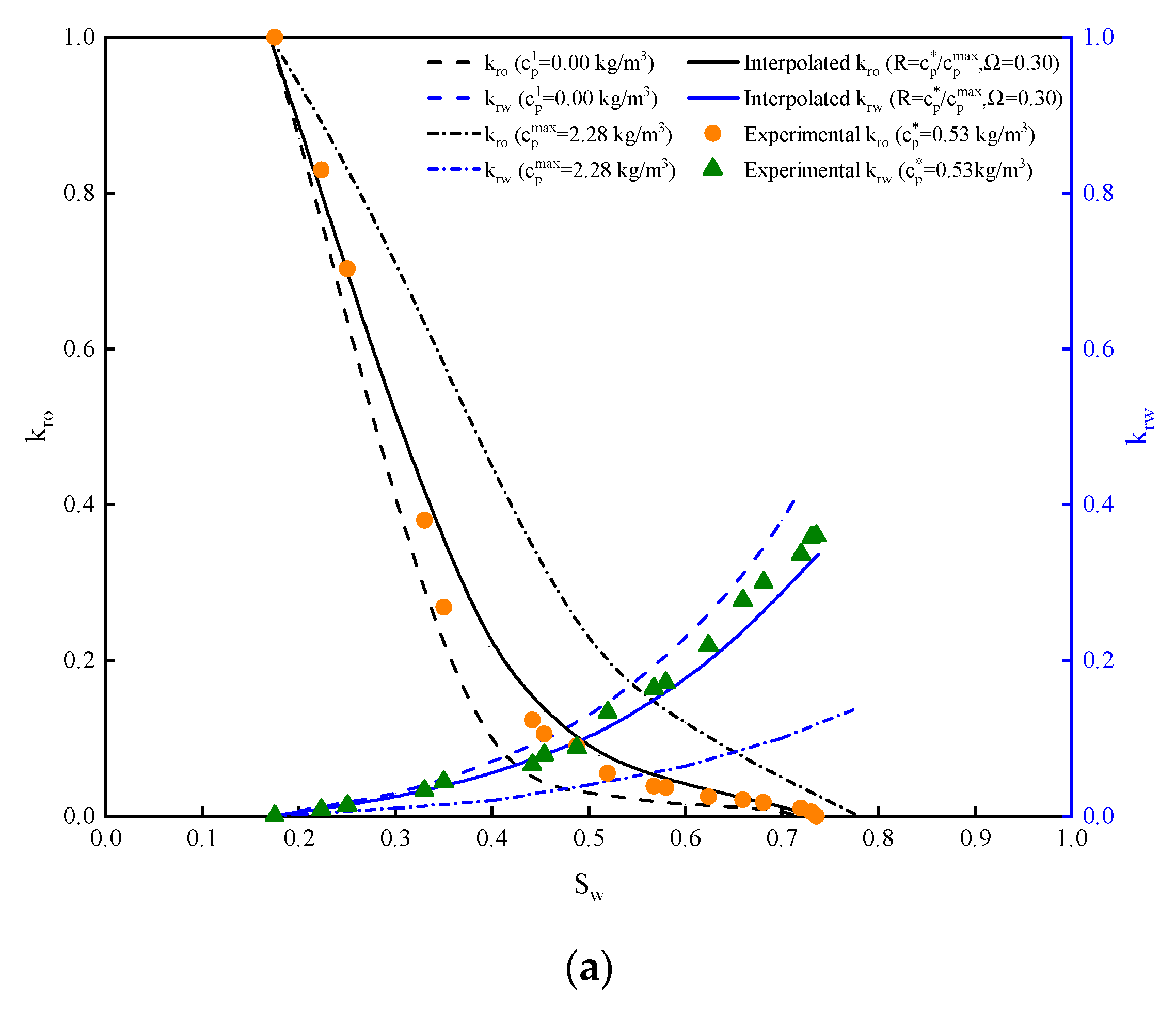
4.1. Cases Study

Based on the methodology and model solution, a mechanism model with a five-spot pattern is applied in this work for the case study (see Figure 5). The basic parameters of the mechanism model and the properties of the polymer solution are respectively shown in

Table 2. The parameters of the basic reservoir’s properties in the case study.

Parameter	Value	Unit
Reservoir dimension	300 × 300 × 10	m
Grid number	25 × 25 × 1	-
Depth	2100	m
Permeability	700 × 700 × 70	mD
Porosity	0.25	-
Initial oil saturation	83.0	%
Initial water saturation	17.0	%
Oil density	850	kg/m3
Water density	1000	kg/m3
Oil formation volume factor	1.16	-
Water formation volume factor	1.05	-
$S_{ipv}$	0.08	-

and Figure 6. The production period of the case study includes three parts: depletion for 15 days, waterflooding for 10 years and polymer flooding for 10 years. In each developmental period, the well’s performances are changed as well. In depletion, the liquid production of the producer (PROD01 well) is set as 30 m3/day, with a 10 MPa limit of the bottom hole pressure (BHP). In the waterflooding and polymer flooding period, the liquid production of the producer increases to 80 m3/day, and the four injectors are switched to inject liquid at 20 m3/day constantly, wherein the liquid is water or polymer solution (${{c}}_{{p}}=2.28 \mathrm{kg}/{{m}}^3$) for the corresponding period.

To discuss the effect of polymer concentration variations on well production in the polymer flooding period, three cases (Base case, Case A and Case B) with different relative permeability curves are evaluated in the simulator (see

Table 3. Model setting of the cases study.

Cases	Treatment of the Relative Permeability Curve in Polymer Flooding
Base Case (ECLIPSE simulator [27])	Curve at ${{c}}_{{p}}=0.00 \mathrm{kg}/{{m}}^3$
Case A	Curve at ${{c}}_{{p}}=2.28 \mathrm{kg}/{{m}}^3$
Case B	Curve calculated by the interpolation factor ${\Omega }_1$
Case C	Curve calculated by the interpolation factor ${\Omega }_2$
Case D	Curve calculated by the interpolation factor ${\Omega }_3$

). The simulated results show that the decrease degree of the water cut in the Base case is the lowest, since it ignores the difference in flow behavior between the water phase and polymer solution (see Figure 7a). In increasing the oil production of the producer, Case A has the largest effect of these three cases (see Figure 7b). This is because the displacement efficiency of the water phase in the reservoir has been overestimated by the oil–polymer solution relative permeability curve when the polymer flooding starts to work. The calculated water cut and the oil production of Case B are between those of the Base case and Case A. Compared with Case A, in the sweeping area of the injected polymer the water saturation in Case B increases with the polymer concentration due to the effects of polymer concentration variations on water flow capability (see Figure 8). Although a similar distribution trend is observed in the Base case, the estimated deviation of the polymer solution’s mobility may lead to inexact predictions. Thus, Case B could describe the flow behavior of the polymer flooding more accurately.

Moreover, Case B, Case C and Case D are applied in this work to study the changing degree of the interpolation factor $\Omega$ with the polymer concentration (see Table 3 and Figure 9). The respective interpolation factors ${\Omega }_1$, ${\Omega }_2$, ${\Omega }_3$ are shown in

Table 4. The interpolation factor in the case study.

${\mathit{c}}_{\mathit{p}}$$/{\mathit{c}}_{\mathit{p}\mathbf{max}}$	${\mathsf{\Omega }}_1 (\mathbf{Case} \mathbf{B})$	${\mathsf{\Omega }}_2(\mathbf{Case} \mathbf{C})$	${\mathsf{\Omega }}_3 (\mathbf{Case} \mathbf{D})$
0.00	0.00	0.00	0.00
0.20	0.20	0.77	0.01
0.40	0.40	0.96	0.04
0.60	0.60	0.98	0.15
0.80	0.80	0.99	0.40
1.00	1.00	1.00	1.00

and Figure 10. The calculation results demonstrate that different $\Omega$ could influence the timing of controlling the water cut and increasing oil production. Thus, the oil–water relative permeability curves dependent on the polymer concentration improve the applicability of the polymer flooding simulation. Further, the interpolation factor $\Omega$ could be set as a flexible parameter in history matching to reflect the interaction between different rock types and different polymer solutions.

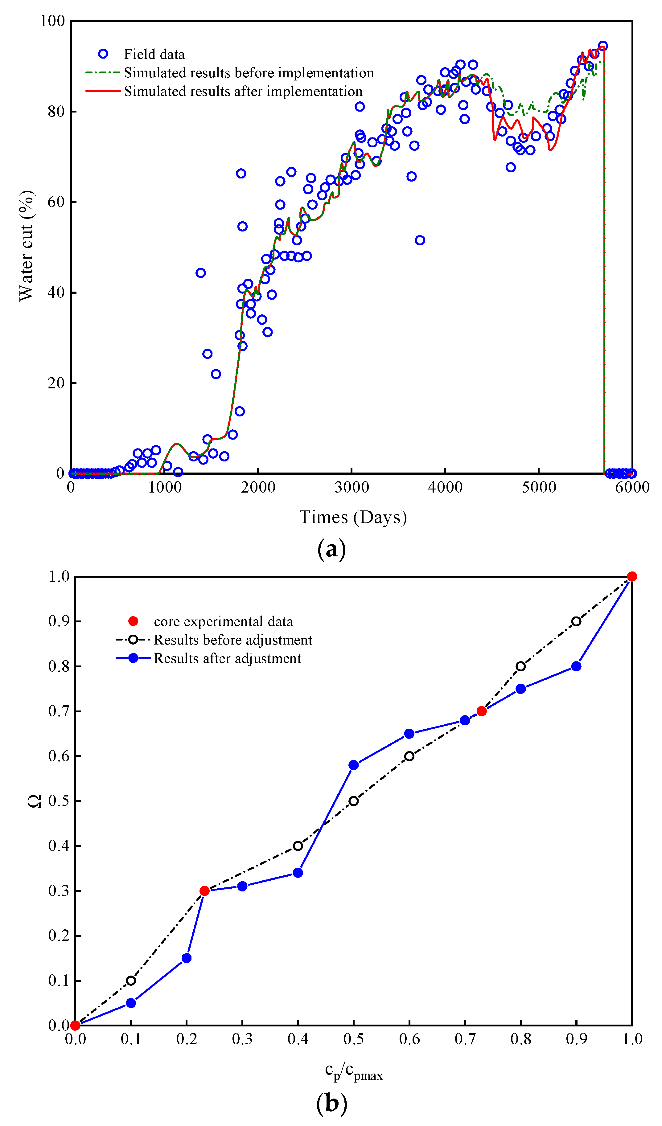
4.2. Field Study

Based on the above analysis of the case study, the oil–water relative permeability curves with polymer concentration variation exhibit a clear difference in the production of the polymer flooding, and the interpolation factor $\Omega$ is set as the adjustable parameter to fit the field data. Here, the production performances of two producers in the Y oilfield are considered to implement the polymer concentration variation in the history matching process. Since the water cut of the main productive zone increases sharply, the Y oilfield employs polymer flooding at 3440 days.

For well S07 and well B12, the water cut matching results of the waterflooding period are within the engineering error. However, the oil–water relative permeability curves for waterflooding could not apply to the history matching of polymer flooding, which is called in this work the simulated results before implementation (see Figure 11a and Figure 12a). To achieve better results, core experimental data of relative permeabilities with different polymer concentrations in the verification section are used to obtain the interpolation factor $\Omega$ (see the red points in Figure 11b and Figure 12b). With these experimental results, more supposed interpolation factors proportional to the normalized polymer concentration ${\mathsf{c}}_{\mathsf{p}}/{\mathsf{c}}_{\mathsf{p}\max }$ are interpolated in order to describe the dynamic oil–water relative permeability. Based on the trial water cut matching results, the supposed $\Omega$ is adjusted dynamically. Figure 11b and Figure 12b illustrate the comparison results of the $\Omega$ adjustment. Correspondingly, the matching results after implementation are closer to the actual field data (see the red lines in Figure 11a and Figure 12a).

5. Conclusions

For polymer flooding, the polymer solution causes an alteration in the oil–water phase flow behavior. This alteration will significantly influence the well performances, such as the water cut and oil production rate. In this study, an interpolation method dependent on polymer concentration is applied to dynamically describe the variation in the oil–water relative permeability curves. The following observations are obtained from this study:

(1)

With the normalized polymer concentration $\mathrm{R}$, a polymer concentration interpolation model for numerical research is proposed to dynamically calculate the corresponding flow mobility of the oil–water phases based on experimental validation.

(2)

Compared with that in the commercial simulator, the proposed interpolation method could more effectively enhance the numerical predictions of the oil production rate and the water cut.

(3)

By combining with the core experimental results, the presented method has been successfully applied in the field history matching of the main productive zone in the Y oilfield, leading to the flexibility improvement of the history matching process.

References

- Raffa, P.; Broekhuis, A.A.; Picchioni, F. Polymeric surfactants for enhanced oil recovery: A review. J. Pet. Sci. Eng. 2016, 145, 723–733. [Google Scholar] [CrossRef]
- Wang, Y.; Cheng, S.; Feng, N.; Xu, J.; Qin, J.; He, Y.; Yu, H. Semi-analytical modeling for water injection well in tight reservoir considering the variation of waterflood—Induced fracture properties—Case studies in Changqing Oilfield, China. J. Pet. Sci. Eng. 2017, 159, 740–753. [Google Scholar] [CrossRef]
- Wang, Y.; Ayala, L.F. Explicit Determination of Reserves for Variable-Bottomhole-Pressure Conditions in Gas Rate-Transient Analysis. SPE J. 2019. [Google Scholar] [CrossRef]
- Van, S.L.; Chon, B.H. Chemical Flooding in Heavy-Oil Reservoirs: From Technical Investigation to Optimization Using Response Surface Methodology. Energies 2016, 9, 711. [Google Scholar] [CrossRef]
- Sheng, J.J.; Leonhardt, B.; Azri, N. Status of Polymer-Flooding Technology. J. Can. Pet. Technol. 2015, 54, 116–126. [Google Scholar] [CrossRef]
- Zhong, H.; Zhang, W.; Fu, J.; Lu, J.; Yin, H. The Performance of Polymer Flooding in Heterogeneous Type II Reservoirs-An Experimental and Field Investigation. Energies 2017, 10, 454. [Google Scholar] [CrossRef]
- Sorbie, K.S. Network Modeling of Xanthan Rheology in Porous Media in the Presence of Depleted Layer Effects. In Proceedings of the 1989 SPE Annual Technical Conference and Exhibition, San Antonio, TX, USA, 8–11 October 1989. [Google Scholar]
- Lopez, X.; Blunt, M.J. Predicting the Impact of Non-Newtonian Rheology on Relative Permeability Using Pore-Scale Modeling. In Proceedings of the SPE Annual Technical Conference and Exhibition, Houston, TX, USA, 26–29 September 2004. [Google Scholar]
- Bo, Q.; Zhong, T.; Liu, Q. Pore Scale Network Modeling of Relative permeability in Chemical flooding. In Proceedings of the SPE International Improved Oil Recovery Conference in Asia Pacific, Kuala Lumpur, Malaysia, 20–21 October 2003. [Google Scholar]
- de Loubens, R.; Vaillant, G.; Regaieg, M.; Yang, J.; Moncorgé, A.; Fabbri, C.; Darche, G. Numerical Modeling of Unstable Waterfloods and Tertiary Polymer Floods into Highly Viscous Oils. SPE J. 2018, 23, 1909–1928. [Google Scholar] [CrossRef]
- Guo, Y.; Zhang, L.; Zhu, G.; Yao, J.; Sun, H.; Song, W.; Yang, Y.; Zhao, J. A Pore-Scale Investigation of Residual Oil Distributions and Enhanced Oil Recovery Methods. Energies 2019, 12, 3732. [Google Scholar] [CrossRef]
- Jingfu, D.; Yunpeng, L.; Xiaofei, J.; Xiaohui, W.; Bin, L. Dynamic Inverting Method for the Relative Permeability Curves in the Stable Polymer Flooding and Its Application. Pet. Geol. Oilfield Dev. Daqing 2017, 36, 106–109. [Google Scholar]
- Wang, Y.; Li, G.; Reynolds, A.C. Estimation of Depths of Fluid Contacts by History Matching Using Iterative Ensemble-Kalman Smoothers. SPE J. 2010, 15, 509–525. [Google Scholar] [CrossRef]
- Hou, J.; Wang, D.; Luo, F.; Li, Z.; Bing, S. Estimation of the Water–Oil Relative Permeability Curve from Radial Displacement Experiments. Part 1: Numerical Inversion Method. Energy Fuels 2012, 26, 4291–4299. [Google Scholar] [CrossRef]
- Bingyan, H.; Xu, C.; Gen, K.; Qiong, L.; Yong, L.; Ke, A. Inverse of parameters of core polymer flooding using iterative ensemble Kalman filter. Prog. Geophys. 2018, 33, 2330–2335. [Google Scholar]
- Liu, Y.; Hou, J.; Liu, L.; Zhou, K.; Zhang, Y.; Dai, T.; Guo, L.; Cao, W. An Inversion Method of Relative Permeability Curves in Polymer Flooding Considering Physical Properties of Polymer. SPE J. 2018, 23, 1929–1943. [Google Scholar] [CrossRef]
- Delshad, M.; Bhuyan, D.; Pope, G.A.; Lake, L.W. Effect of Capillary Number on the Residual Saturation of a Three-Phase Micellar Solution. In Proceedings of the SPE Enhanced Oil Recovery Symposium; Society of Petroleum Engineers: Tulsa, OK, USA, 1986. [Google Scholar]
- Amaefule, J.O.; Handy, L.L. The Effect of Interfacial Tensions on Relative Oil/Water Permeabilities of Consolidated Porous Media. Soc. Pet. Eng. J. 1982, 22, 371–381. [Google Scholar] [CrossRef]
- Jin, M. A Study of Nonaqueous Phase Liquid Characterization and Surfactant Remediation. Ph.D. Thesis, The University of Texas at Austin, Austin, TX, USA, 1995. [Google Scholar]
- Pope, G.A.; Wu, W.; Narayanaswamy, G.; Delshad, M.; Sharma, M.M.; Wang, P. Modeling Relative Permeability Effects in Gas-Condensate Reservoirs with a New Trapping Model. SPE Reserv. Eval. Eng. 2000, 3, 171–178. [Google Scholar] [CrossRef]
- John, A.; Han, C.; Delshad, M.; Pope, G.A.; Sepehrnoori, K. A New Generation Chemical Flooding Simulator. SPE J. 2005, 10, 206–216. [Google Scholar] [CrossRef]
- Han, C.; Delshad, M.; Sepehrnoori, K.; Pope, G.A. A Fully Implicit, Parallel, Compositional Chemical Flooding Simulator. SPE J. 2007, 12, 322–338. [Google Scholar] [CrossRef]
- Guo, C.; Gang, Z.; Yuanle, M.A. Mathematical model of enhanced oil recovery for viscous-elastic polymer flooding. J. Tsinghua Univ. Technol. 2006, 46, 882–885. [Google Scholar]
- Zhenbo, S.; Guo, C.; Gang, S. A new mathematical model for polymer flooding. Acta Pet. Sin. 2008, 29, 409–413. [Google Scholar]
- Jing, W.; Huiqing, L.I.U.; Chaofeng, W.; Haiyang, P. Discussions on some problems about the mathematical model of polymer flooding. Acta Pet. Sin. 2011, 32, 857–861. [Google Scholar]
- Wang, J.; Liu, H.-Q.; Xu, J. Mechanistic Simulation Studies on Viscous-Elastic Polymer Flooding in Petroleum Reservoirs. J. Dispers. Sci. Technol. 2013, 34, 417–426. [Google Scholar] [CrossRef]
- Schlumberger ECLIPSE Reservoir Simulation Software Manuals. 2018.
- Dayong, C.; Yanlai, L.; Na, F.; Hua, Z.; Zhiqiang, Z. Experimental study on variation law of relative permeability curves of polymer flooding. Reserv. Eval. Dev. 2019, 9, 56–59. [Google Scholar]
- Jiang, W.; Zhang, J.; Song, K.; Tang, E.; Huang, B. Study on the surfactant/polymer combination flooding relative permeability curves in Offshore heavy oil reservoirs. In Advances in Materials and Materials Processing IV, PTS 1 and 2; Jiang, Z., Han, J., Eds.; Trans Tech Publications Ltd.: Durnten-Zurich, Switzerland, 2014; Volumes 887–888, p. 53. [Google Scholar]
- Barreau, P.; Lasseux, D.; Bertin, H.; Glenat, P.; Zaitoun, A. An experimental and numerical study of polymer action on relative permeability and capillary pressure. Pet. Geosci. 1999, 5, 201–206. [Google Scholar] [CrossRef]
- Zaitoun, A.; Kohler, N. Two-Phase Flow through Porous Media: Effect of an Adsorbed Polymer Layer. In Proceedings of the SPE Annual Technical Conference and Exhibition, Houston, TX, USA, 2–5 October 1988. [Google Scholar]
- Todd, M.R.; Longstaff, W.J. The Development, Testing, and Application Of a Numerical Simulator for Predicting Miscible Flood Performance. J. Pet. Technol. 1972, 24, 874–882. [Google Scholar] [CrossRef]
- Sorbie, K.S. Polymer retention in porous media. In Polymer-Improved Oil Recovery; Sorbie, K.S., Ed.; Springer: Dordrecht, The Netherlands, 1991; pp. 126–164. [Google Scholar]
- Ruizhong, J.; Yongzheng, C.; Yong, H.; Xin, Q.; Yihua, G.; Jianchun, X. Numerical simulation of polymer flooding considering reservoir property time variation. Fault Block Oil Gas Field 2019, 26, 751–755. [Google Scholar]