A Novel Fault Location Method of a 35-kV High-Reliability Distribution Network Using Wavelet Filter-S Transform

Abstract

Timely and accurate fault location for a 35-kVhigh-reliability distribution network is one of the key technologies to improve the safety and efficiency of distribution network operations. A novel fault location method of 35-kV high-reliability distribution network is proposed in this paper. First, the distributed multipoint fault location model is established based on the power structure of a 35-kV high-reliability distribution network. The distribution of voltage and current traveling waves along the lines is comprehensively considered in this model. Secondly, we analyze the influence of noise interference, analog-digital conversion frequency, and conversion bits on the location accuracy. The simulation method of noise and analog-digital conversion is proposed based on simulated samples. Then, a wavelet filter is used to reduce the influence of noise on the calibration of the traveling wave arrival time, and matrix modulus of S transform is used to identify the arrival time for the wave. Finally, the simulation model of a 35-kV high-reliability distribution network is established to analyze the location accuracy in the case of single-phase to ground via resistance, two-phase short-circuit to ground via resistance, and three-phase short-circuit faults. The simulation results indicate that the proposed method has high location accuracy under the above fault conditions.

1. Introduction

The distribution network plays an important supporting role in promoting economic and social development [1]. Due to the large volume of equipment and wide coverage, it is difficult to find and repair faults in time. Therefore, timely and accurate fault location of the distribution network is an important foundation to ensure the safe and reliable operation of the network [2].

At present, scholars have studied the application of wavelet transform, Hibbert–Huang transform and S transform in traveling wave fault location. Hu et al. [3] studied the principle of double-ended traveling wave fault location for transmission lines. The application of wavelet transform in traveling wave fault location is analyzed. Han et al. [4] formed a switch state matrix based on the adjacency matrix and mapped the fault current distribution into a current state matrix. The method unified the two matrices into a fault state matrix to reflect the fault state of the all-parallel autotransformer railway systems (AARS). Ji et al. [5] analyzed the application of the traveling wave fault location method based on wavelet transform in the 10-kV system. The algorithm of average wave velocity refraction is proposed. The accuracy of the proposed method is verified by simulation. Deng et al. [6] considered the wave speed difference of an overhead line-cable hybrid line. The technology of wave feature matching was used to achieve accurate fault location of hybrid transmission lines. Xiong et al. [7] used the Hilbert–Huang transform to capture the traveling wave of an all-parallel autotransformer (AT) electric railway system. The effective identification of the voltage traveling wave head was defined by the high-frequency wave trap connected between the horizontal lines. Li et al. [8] used S transform to independently analyze the signal amplitude changes of each frequency component. The moment of signal change is judged based on the amplitude-frequency characteristics of a transient traveling wave. The fault position is defined by combining the principle of double-ended ranging. Qian et al. [9] used S transform to capture the arrival time of the traveling wave. The fault section is determined by eliminating roads one by one. The multi-terminal line fault location was completed based on the section result and double-terminal ranging principle. Xie et al. [10] proposed the combination of variational modal decomposition and S transform to complete the feature extraction of the traveling wave under a strong noise background. The effectiveness of the proposed method under a strong noise background was verified by simulation. Dai et al. [11] combined S transform with a particle swarm algorithm to obtain preprocessed voltage data. The global search capability of the particle swarm algorithm was used to solve the optimal solution of the location objective function to determine the fault location. Pang et al. [12] used the generalized S transform to obtain the time–frequency transformation matrix of the transient zero-sequence current and the energy of each frequency band. The maximum energy margin was served to locate the single-phase ground fault interval of the distribution network.

The mentioned literature fully explain the principle of fault location and the application of S-transform. However, there are the following problems. (1) Less analysis of the actual operation noise of the lines, especially the influence of the environment and measurement noise on the fault location accuracy. The impact of environmental and measurement noise on the traveling wave is similar to the change caused by the line fault. The singular feature of the fault traveling wave might be covered by the noise signal, which makes it impossible to accurately identify the fault position. (2) The existing research seldom considers the influence of analog–digital conversion of the traveling wave sampling device on data accuracy. In fact, the accuracy of the sampled data is reduced by the analog–digital conversion. The singular characteristics of traveling waves caused by line faults are weakened. It is more likely for the traveling wave singularities to be covered in noise signals. The accuracy of the fault location will be lower. According to the shortage of the mentioned literature, environment and measurement noise is combined with ideal traveling wave data in this paper. The influence of noise on the fault location accuracy is fully analyzed. A formula for the analog-to-digital conversion is established. In order to obtain high location accuracy, the method of wavelet filter-S transform is proposed. The impact of noise can be reduced by a wavelet filter. The S transform is used to define the arrival time of the fault wave. S-transform has more anti-noise ability. The result of the S transform is a two-dimensional complex matrix. It can provide rich time–frequency information and fine fault feature, which is beneficial to improve location accuracy in the distribution network [13].

On the basis of the above research, the distributed multi-point location model suitable for a 35-kV high-reliability distribution network is established in this paper. The identification method of the traveling wave arrival time based on wavelet filter-S transform is proposed, which effectively reduces the impact of environmental and measurement noise and analog-digital conversion on the location accuracy. The simulation model of the 35-kV high-reliability distribution network is established with reference to the design parameters of certain domestic railways. Fault conditions including single-phase grounding through transition resistance, two-phase short-circuit grounding through transition resistance, and three-phase short-circuits are simulated to verify the effectiveness of the method proposed in this article. The main fault type of the distribution network is a short-circuit fault, which can be divided into single-phase short-circuit, two-phase short-circuit, and three-phase short-circuit. The 35-kV high-reliability distribution network is an isolated neutral system. The short-circuit current and fault wave characteristics are not obvious. When the lines are grounded through transition resistance, short-circuit current and fault wave features are further weakened [14]. Therefore, three types of faults are selected in this paper including single-phase grounding through transition resistance, two-phase short-circuit grounding through transition resistance, and three-phase short-circuit. The short-circuit current and wave features of the above three faults are the least obvious. Location accuracy under the above three types of faults is highly representative.

2. Principle of Fault Location for a 35-kV High-Reliability Distribution Network

In this section, the actual power supply of a 35-kV high-reliability distribution network and the principle of double-ended location are considered. The distributed multi-point location model which comprehensively contains the voltage and current traveling waves is established. The influence of the analog–digital conversion frequency, the number of conversion bits, and the environment and measurement noise on the identification of the traveling wave arrival time is analyzed. The simulation methods of analog–digital conversion and noise interference based on simulation data are proposed.

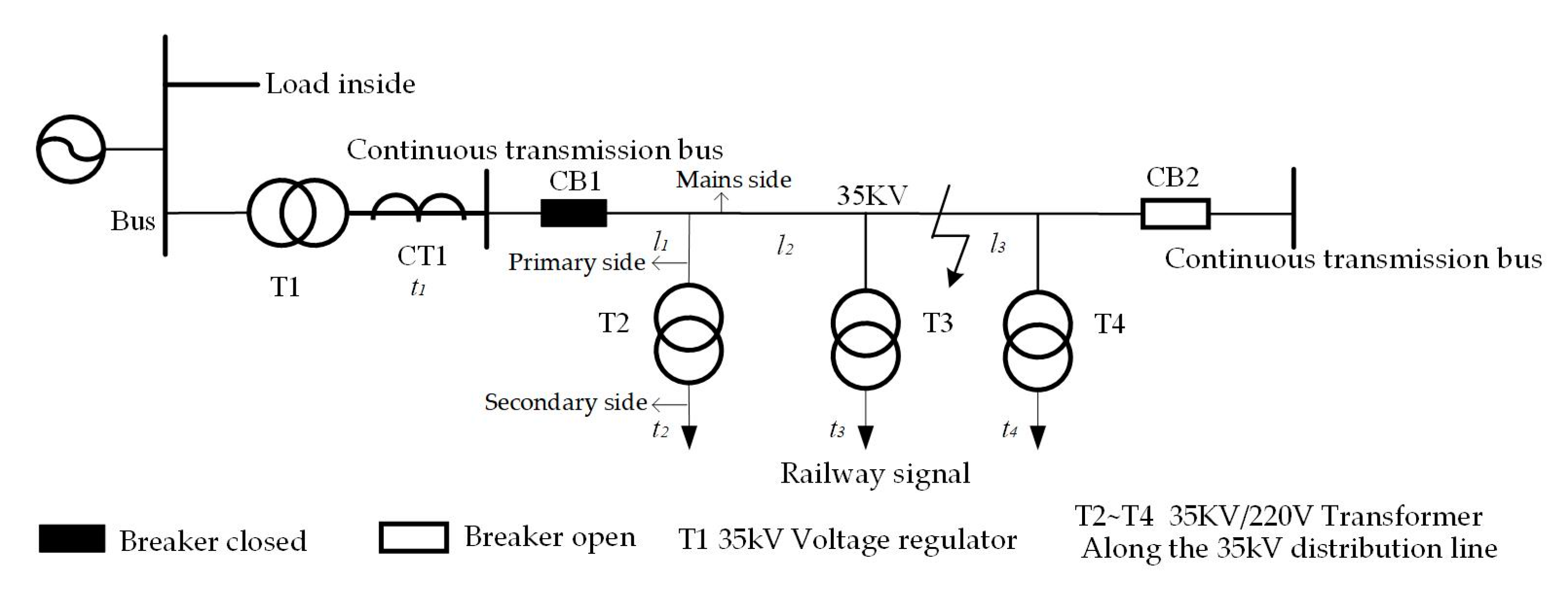
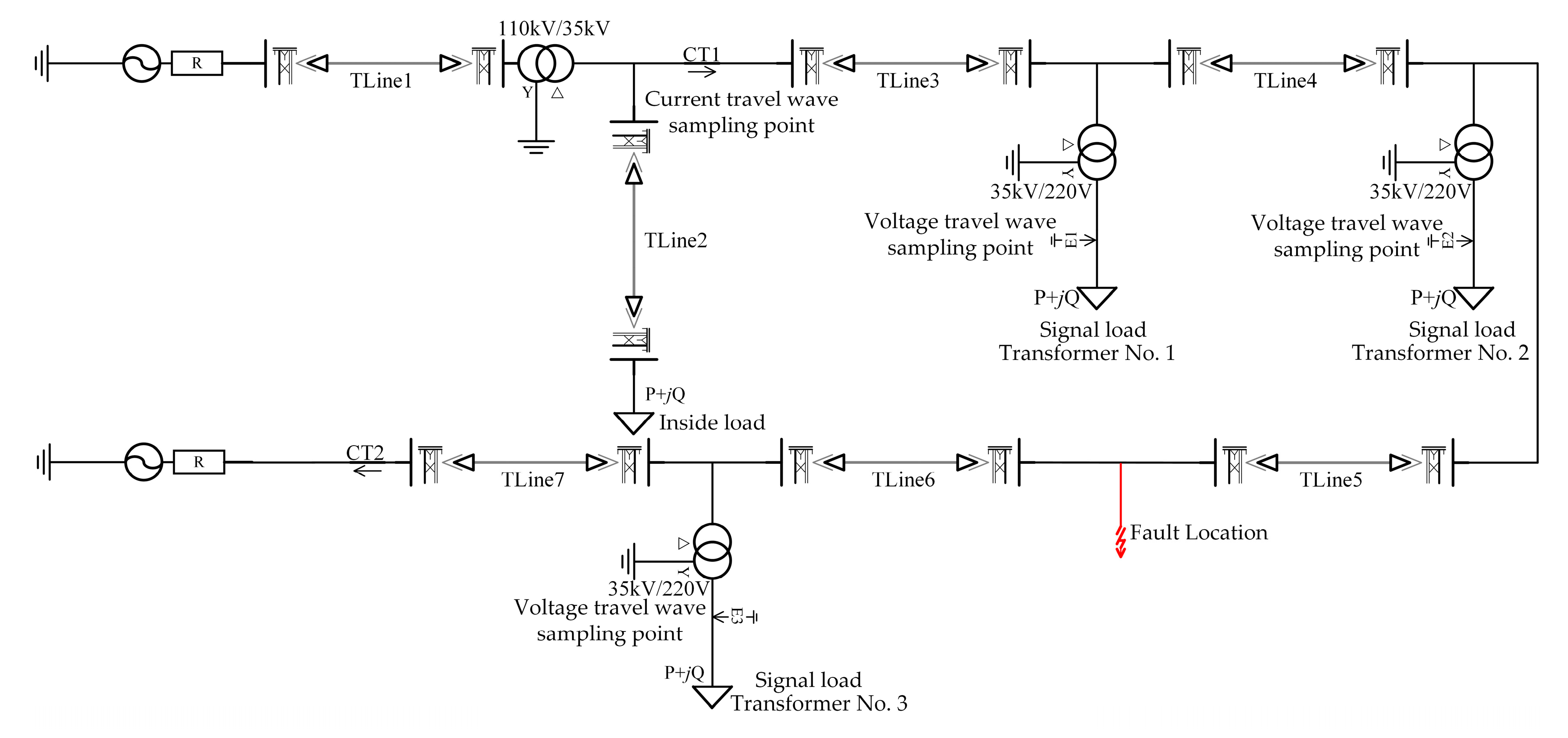
2.1. Structures of 35-kV High-Reliability Distribution Network

The 35-kV high-reliability distribution network is an important part of the railway power system, which provides a reliable power supply for railway signal equipment. The 35-kV high-reliability distribution network consists of automatic blocking and continuous transmission lines (ABCTLs). The automatic blocking lines mainly supply power for blocking signal loads. The continuous transmission lines offer electricity for railway signal, communication, and other railway integrated electricity. The distribution network of the same power supply section is both double-ended power sources. It is a single power supply during normal operation. Two neighboring power distribution stations supply power to the 35-kV high-reliability distribution network. One distribution station is used for power supply and the other is the backup power [15]. The schematic diagram of the 35-kV high-reliability distribution network is shown in Figure 1.

2.2. Principle Simulation of Double-Ended Location

Fault location can be roughly divided into the fault indicator method, injected signal tracking method, impedance method, and traveling wave method according to the principle. The traveling wave method has been widely used because of high location accuracy and little influence from external factors [16]. The traveling wave method can be roughly divided into single-ended location and double-ended location based on the number of measurement terminals. In an actual fault location, single-ended ranging was affected by the complex operating environment and noise. The reflected wave from the opposite terminal cannot be accurately identified. Therefore, the fault location was completed in this paper based on the principle of a double-ended location. The absolute time difference of the fault traveling wave arrival at both ends of the line was used to obtain the fault position in double-ended locations [17]. The location principle is shown in Figure 2. The calculation method is Equation (1).

$$\begin{array}{l}{D}_{\mathrm{M}}=\frac{\left(t_{\mathrm{M}}-t_{\mathrm{N}}\right)v+l_{\mathrm{MN}}}{2}\hfill \\ D_{\mathrm{N}}=\frac{\left(t_{\mathrm{N}}-t_{\mathrm{M}}\right)v+l_{\mathrm{MN}}}{2}\hfill \end{array}$$

(1)

where t_M, t_N is the time when the fault traveling wave reaches both ends of the line, v is the wave speed, l_MN is the total length of the line, D_M is the distance from the fault point to the M terminal, and D_N is the distance from the fault point to the N terminal.

The key to a double-ended location is the time synchronization of the sampling devices at both ends of the line. GPS synchronous timing was used for time synchronization in this article. GPS timing can achieve nanosecond synchronization of the devices at both ends, which can minimize the location error caused by time asynchrony [18].

2.3. Model of Distributed Multi-Point Location

Although the 35-kV high-reliability distribution network is the structure of a dual power supply, it has a single power supply during normal operation. The end breaker of the line is open, which means the end of line is open. The current traveling wave signal cannot be collected by the current transformer at the end. The single current traveling wave cannot be used for a double-ended location as shown in Figure 3.

The 35-kV/220 V transformers are installed along 35-kV high-reliability distribution networks to supply power for the railway signal system. Theoretical research shows that the transformer can effectively transfer the traveling wave. So, the voltage traveling wave on the secondary side of the transformer can be collected for fault location [19]. The impact of the transformer transmission on the arrival time of the traveling wave was fully considered. A phase A grounding fault was simulated. The duration was 0.01 s, the sampling step was 0.5 μs, the simulation time was 0.15 s, and the time of fault occurrence was 0.092 s. The simulation model was also a 35-kV high-reliability distribution network. The voltage and current traveling wave data from 0.07 to 0.15 s was selected. The secondary side voltage traveling wave, primary side current traveling wave, and mains side current traveling wave of the T2 transformer were collected as Figure 4. The secondary side, primary side, and mains side of T2 transformer are indicated in Figure 3.

The initial arrival time of the traveling wave shown in Figure 4 is determined based on the wavelet transform, as shown in

Table 1. Arrival time of the traveling wave at different measuring points.

Sampling Point	Secondary Side Voltage Traveling Wave of T2 Transformer	Primary Side Current Traveling Wave of T2 Transformer	Mains Side Current Traveling Wave of T2 Transformer
Arrival time/s	0.092502	0.092502	0.092502

.

It can be seen from Table 1 that the transformer could effectively transfer the traveling wave. The arrival time of the secondary side voltage traveling wave was consistent with the primary side and the mainline side current traveling wave. The equal times reflect that transformers cannot affect the arrival time of the traveling wave. So, the arrival time determined by the current traveling wave and the voltage traveling wave along the lines was credible.

Based on the principle of double-end location, the current traveling wave and the voltage traveling wave along the lines were comprehensively used. The distributed multi-point location model suitable for a 35-kV high-reliability distribution network was established [20]. The time difference between both ends of the non-faulty line was selected to calculate the wave speed. The time difference between both ends of the faulty line was used to define the fault location [21]. The current traveling wave was collected by the current transformer (CT) at the head or end of the line. The voltage traveling wave is obtained on the secondary side of the 35-KV/220 V transformer of T2~T4. The secondary side voltage of the transformer is 220 V, which can be directly connected to the traveling wave sampling device. The construction investment caused by the additional installation of voltage or current transformers was avoided. The difficulty of the project was reduced.

For example, the time t₂ and t₃ at both ends of the non-faulty line was used to obtain the wave speed. The t₃ and t₄ was used to calculate the distance between the fault point and the T3 transformer. The formula is as follows:

$$\begin{array}{c}v=\frac{l_2}{t_2-t_3}\\ D_2=\frac{(t_3-t_4)\cdot v+l_3}{2}\end{array}$$

(2)

where v is the speed of the traveling wave. t₂ is the arrival time defined by the secondary side voltage traveling wave of T2 transformer. t₃ is the arrival time defined by the secondary side voltage traveling wave of T3 transformer. t₄ is the arrival time defined by secondary side voltage traveling wave of T4 transformer. l₂ is the distance between T2 transformer and T3 transformer. l₃ is the distance between T3 transformer and T4 transformer. D₂ is the distance between the fault position and the T2 transformer.

In addition, (t₁, t₂, t₄) and (t₁, t₃, t₄) can be selected for location. The average of the three location results can be calculated to minimize the ranging error. The formula is as follows:

$$D_2=\left[\frac{(t_3-t_4)\cdot \frac{l_2}{t_2-t_3}+l_3}{2}+\left(\frac{(t_2-t_4)\cdot \frac{l_1}{t_1-t_2}+(l_2+l_3)}{2}-l_2\right)+\frac{(t_3-t_4)\cdot \frac{l_1+l_2}{t_1-t_3}+l_3}{2}\right]/3$$

(3)

where t₁ is the arrival time defined by the current traveling wave of CT1. l₁ is the distance between the CT1 and T2 transformer.

The wave speed is obtained based on the actual transmission time of the traveling wave in the model of distributed multi-point location, which avoids that the traditional wave speed calculation method only considers the line parameters and fails to analyze the influence of the line environment on the wave speed. The location error caused by inaccurate wave speed measurement is reduced.

2.4. Analog–Digital Conversion and Noise Interference

2.4.1. Frequency and Bits of Analog–Digital Conversion

The influence of analog–digital conversion frequency and bits on location error was seldom considered in the present literature. The data were rounded by analog–digital conversion, which reduced the difference between sampling points. The singular characteristics of the traveling wave were weakened. So, the identification difficulty of traveling wave arrival time was improved. In this paper, the analog–digital conversion frequency was 2 MHz and the sampling interval was 0.5 μs. The higher frequency can reduce the location error caused by the interval. It is assumed that the faulty wave travels at the speed of light. The error caused by the sampling interval is as Equation (4).

$$d_{error}=v_{light}\times t_{sample}=3\times {10}^8\mathrm{m}/\mathrm{s}\times 0.5\mathsf{\mu }\mathrm{s}=150\mathrm{m}$$

(4)

where $v_{light}$ is the speed of light, $t_{sample}$ is sampling interval and $d_{error}$ is location error. From Equation (4), it can be seen that the location error is within 150 m, which ensures the accuracy of fault location.

In the actual location, the accuracy of sampled data was limited by analog–digital conversion bits. Higher conversion bits can retain the singular characteristics of the fault traveling wave to the maximum, and the influence of noise signals on the fault location can be reduced. A 16-bit analog–digital conversion is used to obtain more accurate traveling wave data in this paper, which is helpful for subsequent noise filters.

The 2-MHz frequency and 16-bit analog-digital conversion were achieved based on the STM32H7 series of high-performance microcontroller units (MCUs) with the advanced risc machine (ARM) Cortex-M7 core. The processor frequency can reach 480 MHz, which was able to meet the hardware requirements of fault location.

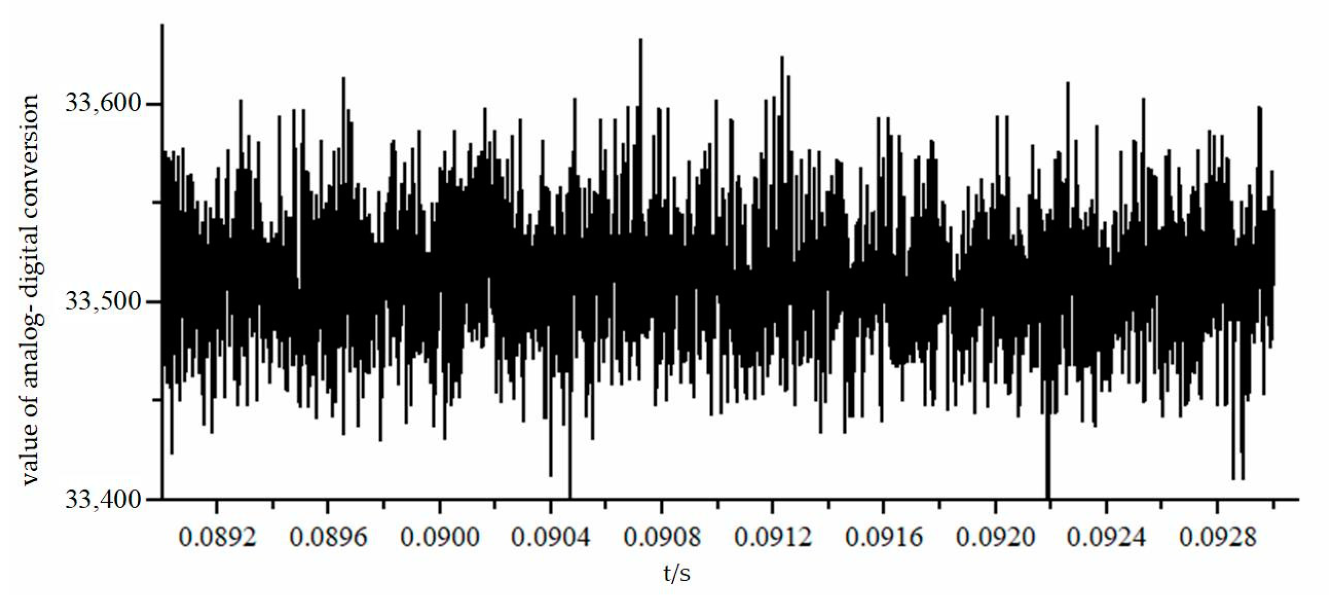
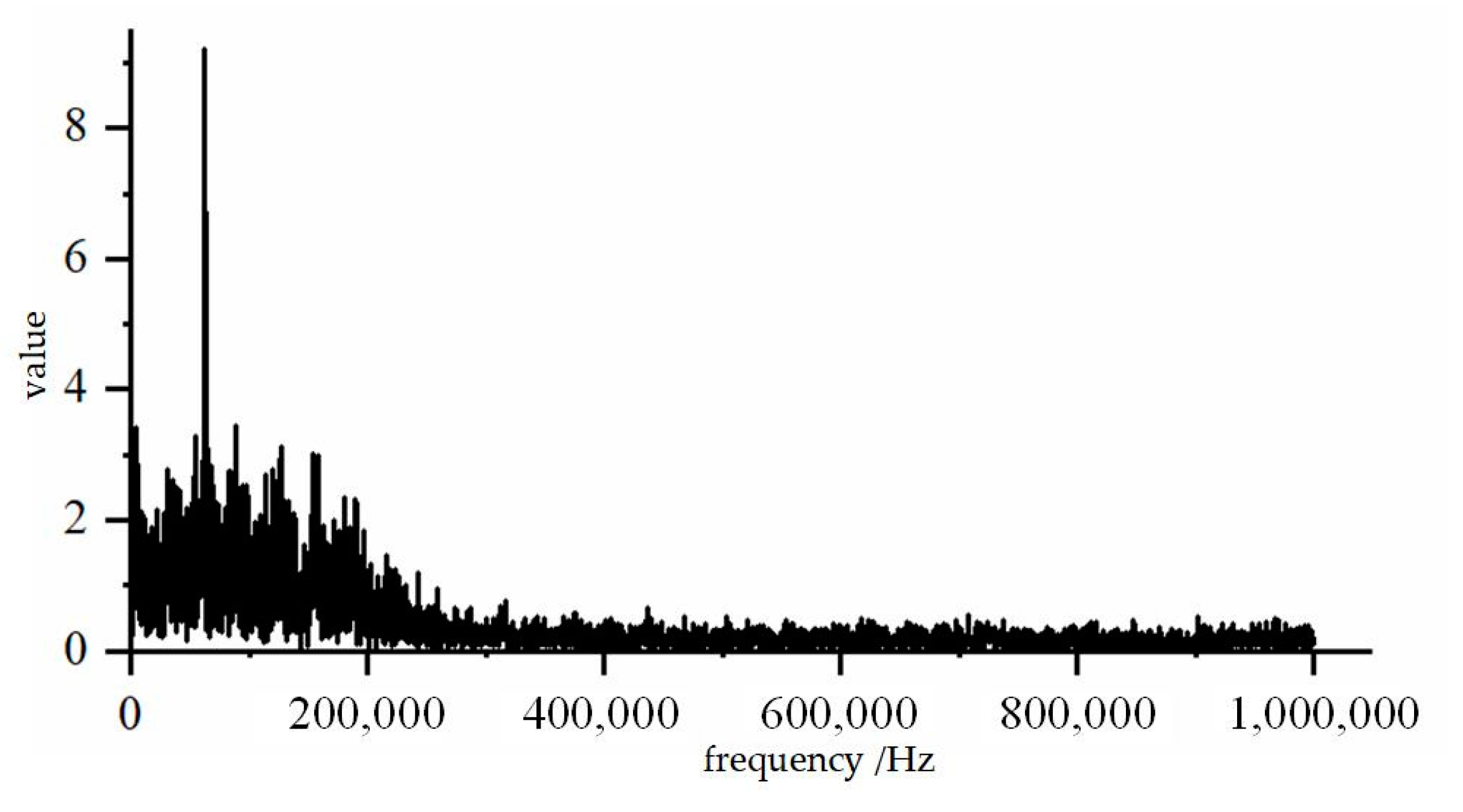
2.4.2. Noise Interference

The line fault wave will inevitably be interfered with by noise. High-frequency noise not only affects the mode value of the traveling wave but also covers the traveling wave singularity. It is impossible to calibrate the arrival time of a traveling wave according to the maximum value of the traveling wave mode [2]. The following takes the noise signal collected by the traveling wave sampling device as an example to illustrate the influence of environment and measurement noise on the traveling wave signal. The noise signal was actual data from a 35-kV high-reliability distribution network, which was collected by a traveling wave sampling device. The device has the same analog–digital conversion frequency and as previously mentioned in this paper. The noise waveform obtained based on the actual distribution network is shown in Figure 5.

It can be seen from Figure 5 that the environmental and measurement noise had a sharp change, which was similar to an uninterrupted pulse signal. The frequency spectrum of the noise signal was obtained by fast Fourier transform to analyze the frequency range of the noise signal, as shown in Figure 6.

It can be seen from Figure 6 that the environmental and measurement noise signals had a higher amplitude within 200 kHz, while the frequency of the fault traveling wave of the ABCTLs was distributed in approximately 10 kHz–100 kHz [22]. Therefore, the two signals were aliased. The influence of noise signals on the calibration of the traveling wave arrival time cannot be ignored.

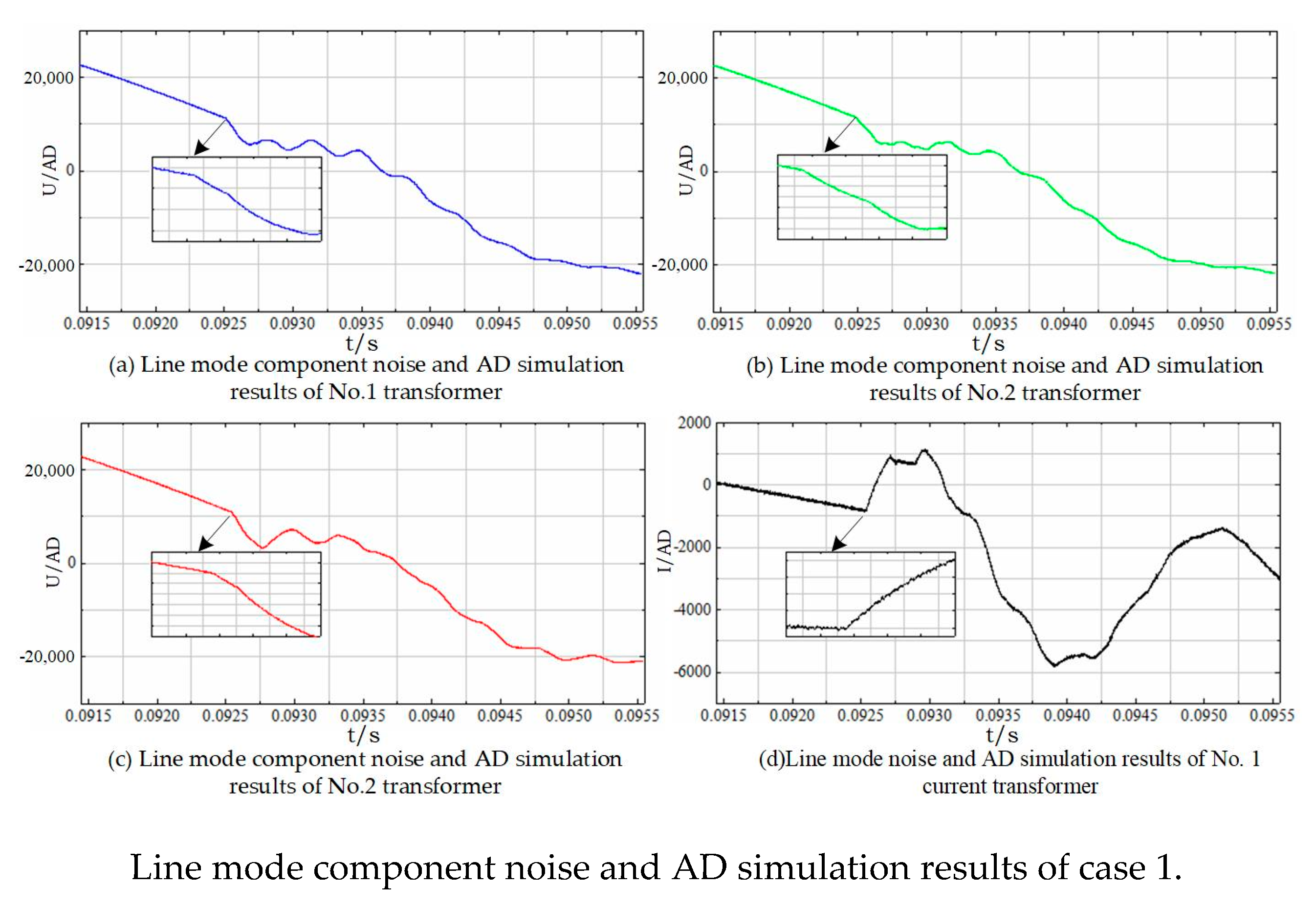
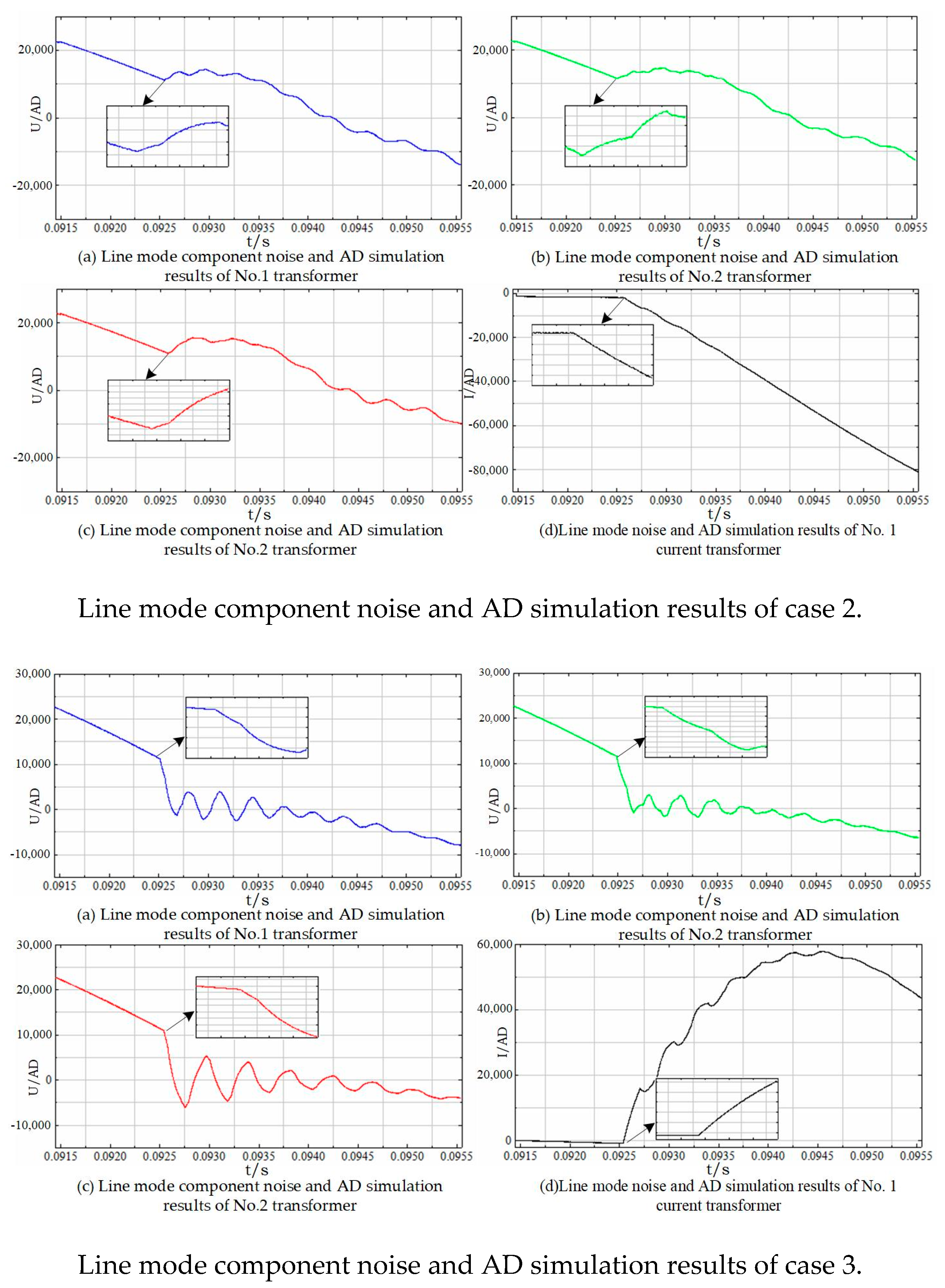
2.4.3. Simulation of Analog–Digital Conversion and Noise Interference

In order to fully reflect the influence of the analog–digital conversion on the location accuracy, the simulated data was converted based on the principle of analog–digital conversion. The conversion formula is as follows.

$$Dat{a}_{\mathrm{ADC}}=\mathrm{INT}(dat{a}_{\mathrm{sim}}\times M/N)+M$$

(5)

where $dat{a}_{\mathrm{sim}}$ is the simulation data, $Dat{a}_{\mathrm{ADC}}$ is the analog-digital conversion simulation data, INT(x) is the rounding function, $M=2^{16}/2=32768$ considering the unipolar analog–digital conversion, N is the short-circuit current or voltage multiple of transformers.

The noise signal was superimposed on the obtained simulation data to fully reflect the influence of noise on the location accuracy. The expression is as follows:

$$Dat{a}_{\mathrm{ADC}+\mathrm{noise}}=Dat{a}_{\mathrm{ADC}}+Dat{a}_{\mathrm{noise}}$$

(6)

3. Calibration of Traveling Wave Arrival Time Based on Wavelet Filter-S Transform

It can be seen that there was aliasing between the noise frequency band and the line fault traveling wave frequency according to the above analysis. The traditional signal filter method was used to separate the useful signal and the noise signal in the frequency domain which was helpful to smooth the noise. However, the method also removed the useful components of the traveling wave signal, which greatly affected the location accuracy. In this section, the arrival time calibration method of traveling wave is proposed based on wavelet filter-S transform. The method was used to determine the arrival time of the traveling wave.

3.1. Wavelet Filter

The research in Section 2.4.2 showed that the traditional digital filter method removed the useful components in the traveling wave due to the aliasing between the noise frequency and the line fault traveling wave frequency. The wavelet filter decomposed various frequency components in the signal into non-overlapping frequency bands. The wavelet transform modulus maximum of the fault traveling wave increased proportionally with the increase of the scale. At the same time, the wavelet transform modulus maximum of the noise decreased. This feature can effectively distinguish the noise signal from the traveling wave signal [23]. Therefore, based on the wavelet transform algorithm, all small-scale high-frequency components were discarded. Large-scale high-frequency components were processed by threshold denoising. Then, the signal was reconstructed which was used for S transform to calibrate the arrival time of the traveling wave.

Threshold denoising processing methods that are commonly used contain hard threshold processing, soft threshold processing, and percentage threshold processing. In order to maximize the elimination of noise signals, soft threshold processing was used [24], as shown in Equation (7).

$$Y=\{\begin{array}{ll}0,& x<0\\ \mathrm{s}ign(x)\cdot (\left|x\right|-T),& x\ge 0\end{array}$$

(7)

where T is the threshold, sign(x) is the sign function that is expressed as the following Equation (8).

$$sign(x)=\{\begin{array}{r}1\begin{array}{cc},& x>0\end{array}\\ 0\begin{array}{cc},& x=0\end{array}\\ -1\begin{array}{cc},& x<0\end{array}\end{array}$$

(8)

The threshold was determined by improving the general threshold selection method, the formula is as follows.

$$T=\sigma \sqrt{2\mathrm{In}(N)}$$

(9)

where $\sigma$ is the noise standard deviation, N is the number of sampling points. As the scale increased, the threshold was reduced by approximately $2^{-1/2}$ [24]. The threshold also needed to be adjusted according to the actual noise situation.

3.2. Model of S Transform

S transform has a frequency-dependent resolution. Its time window width changes inversely with frequency, which has a higher time resolution in the high-frequency part than the wavelet transform [25].

The S transform $S\left(\tau ,f\right)$ of the non-stationary signal x(t) is defined as follows:

$$\begin{array}{c}S(f,\tau )={\displaystyle {\int }_{-\infty }^{+\infty }x(t)\omega \left(\tau -t,f\right)e^{-j2\pi ft}}dt\\ \omega \left(\tau -t,f\right)=\frac{\left|f\right|}{\sqrt{2\pi }}{e}^{\left|\frac{-f^2{(\tau -t)}^2}{2}\right|}\end{array}$$

(10)

where $\omega (\tau -t,f)$ is the Gaussian window, $\tau$ is the position parameter of the Gaussian window on the time axis t, f is the frequency, j is the imaginary unit. S transform can be regarded as the phase correction of the wavelet transform, which can be derived from the wavelet transform and Fourier transform. The result is shown in Equation (11).

$$S(\tau ,f)={\displaystyle {\int }_{-\infty }^{+\infty }X(\upsilon +f)e^{-\frac{2{\pi }^2{\upsilon }^2}{f^2}}}{e}^{j2\pi \tau \upsilon }d\upsilon$$

(11)

In the Equation, $f\ne 0$. S transform can be calculated by FFT. The discrete form of S transform can be obtained as follows:

$$\begin{array}{c}S\left[m,n\right]={\displaystyle \sum _{k=0}^{N-1}X\left[n+k\right]e^{-2{\pi }^2{k}^2/n^2}{e}^{j2\pi km/N}\begin{array}{cc},& n\ne 0\end{array}}\\ S\left[m,n\right]=\frac{1}{N}{\displaystyle \sum _{k=0}^{N-1}x\left[k\right]}\begin{array}{cc},& n=0\end{array}\\ X[n]=\frac{1}{N}{\displaystyle \sum _{k=0}^{N-1}x\left[k\right]}{e}^{-j2\pi kn/N}\end{array}$$

(12)

According to the actual requirements of fault location, the discrete form of S transform is corrected to obtain the practical discrete form of S transform as Equation (13).

$$\begin{array}{c}S\left[m\Delta f,n\Delta t\right]={\displaystyle \sum _{k=0}^{N-1}X\left[n+k\right]e^{-2{\pi }^2{k}^2/n^2}{e}^{j2\pi km/N}\begin{array}{cc},& n\ne 0\end{array}}\\ S\left[m\Delta f,0\right]=\frac{1}{N}{\displaystyle \sum _{k=0}^{N-1}x\left[k\right]}\begin{array}{cc},& n=0\end{array}\end{array}$$

(13)

where $\Delta f\Delta t$ are frequency resolution and time resolution respectively, $\Delta t$ is determined by the sampling frequency, $m\Delta f$ should meet the maximum and minimum sampling frequency limits as follows:

$$f_{\min }\le m\Delta f\le f_{\max }$$

(14)

where $f_{\max }$ should meet Nyquist sampling theorem.

N are the discrete signal sampling points. The transform result is a complex time–frequency matrix with n + 1 rows and m columns. The column corresponds to the sampling time point and the row corresponds to the frequency. The first row corresponds to the DC component in the signal. The frequency difference between neighboring rows is shown as Equation (15).

$$\frac{\left(f_{\max }-f_{\min }\right)\times f_s}{N\times \Delta f}$$

(15)

In the formula, f_s is the sampling frequency, N is the number of sampling points. The frequency corresponding to the nth row is as follows.

$$f_n=\frac{\left(f_{\max }-f_{\min }\right)\times f_s}{N\times \Delta f}n$$

(16)

The minimum sampling interval is as Equation (17).

$$T_s=\frac{\pi +1}{2\pi f_s}$$

(17)

The S modulus matrix is obtained by modulating each element of the S transform result. The column vector represents the amplitude–frequency characteristic of the signal at a certain moment. The row vector represents the time domain distribution of the signal at a certain frequency. In order to obtain the fine time–domain distribution of the fault traveling wave at different frequencies, the sampling interval was selected according to the minimum time interval.

The arrival time of the traveling wave was determined based on the time domain distribution of different frequencies in the S-mode matrix. According to the line fault traveling wave frequency range (approximately 10–100 kHz), the S-mode matrix value was selected in this range. The moment corresponding to the maximum value of the modulus at different frequencies will be defined. The average method was used to obtain the unique modulus maximum value corresponding moment as the final fault traveling wave arrival time. The moment was substituted into Equation (3) to calculate the fault position.

3.3. Steps of Fault Location

Based on the above research, the specific steps of wavelet filter-S transform applied were as follows.

(1)

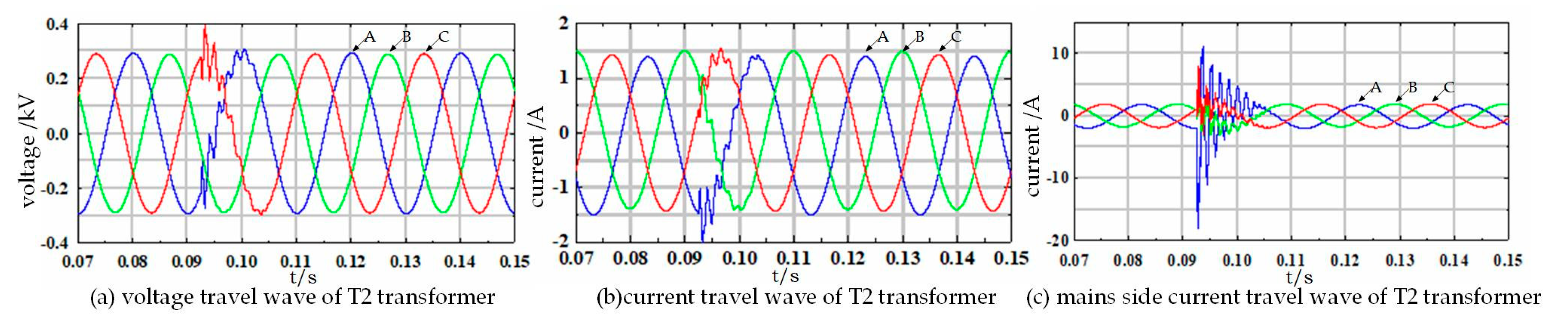
Simulation model of 35-kV high-reliability distribution network was established to collect the voltage and current traveling wave signals. Then, a total of 4 ms traveling wave data was stored for fault location. The three-phase voltage and current traveling waves were converted based on Equations (5) and (6) and mixed in noise.

(2)

The three-phase traveling wave data was carried out by Karen Bell transformation. The formula is shown in Equation (18) to obtain the linear and zero-mode components [26]. As the zero-mode component only exists in ground faults, the line-mode component was used for fault location [27];

$$\begin{array}{c}\left[\begin{array}{c}{I}_{\alpha }\\ I_{\beta }\\ I_0\end{array}\right]=\frac{1}{3}\left[\begin{array}{ccc}1& -1& 0\\ 1& 0& -1\\ 1& 1& 1\end{array}\right]\left[\begin{array}{c}{I}_a\\ I_b\\ I_c\end{array}\right]\\ \left[\begin{array}{c}{U}_{\alpha }\\ U_{\beta }\\ U_0\end{array}\right]=\frac{1}{3}\left[\begin{array}{ccc}1& -1& 0\\ 1& 0& -1\\ 1& 1& 1\end{array}\right]\left[\begin{array}{c}{U}_a\\ U_b\\ U_c\end{array}\right]\end{array}$$

(18)

(3)

The line modulus component obtained by the Karen Bell transform was used for the wavelet filter. The wavelet filter was based on the threshold denoising method, and the threshold was determined by the general threshold method.

(4)

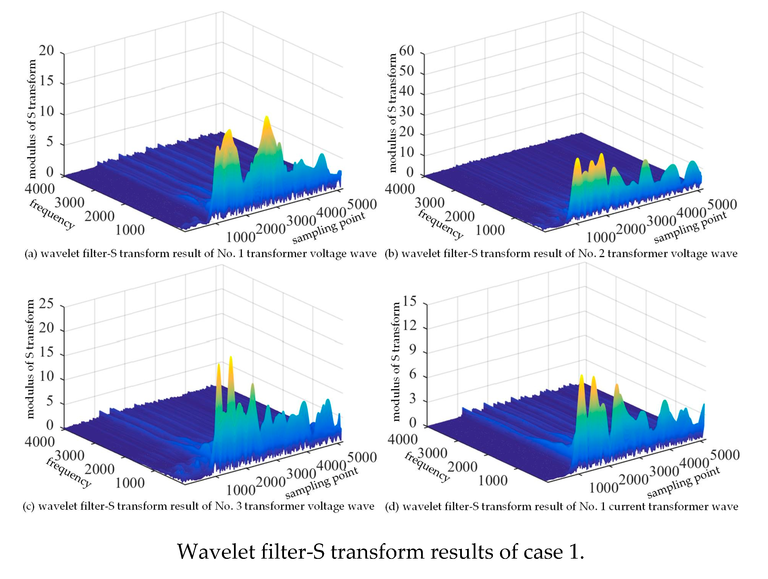
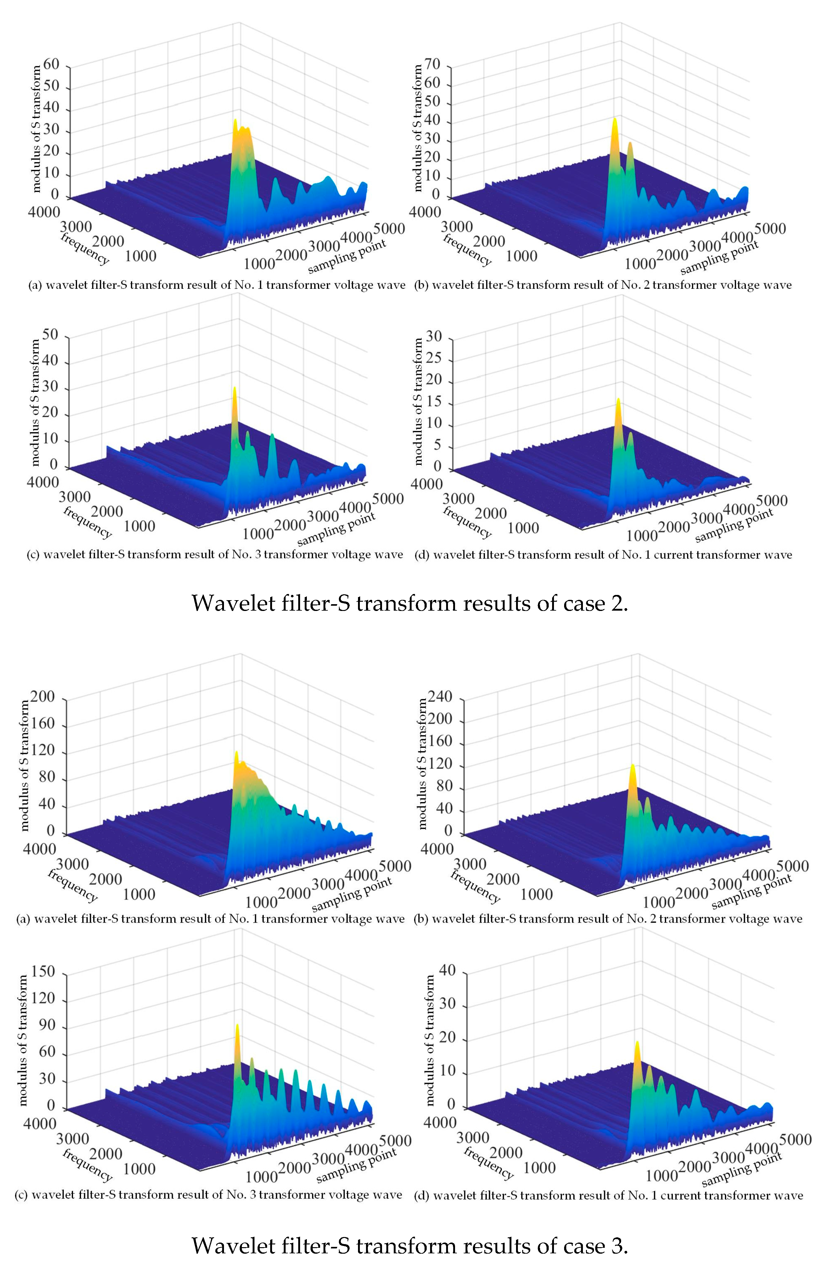
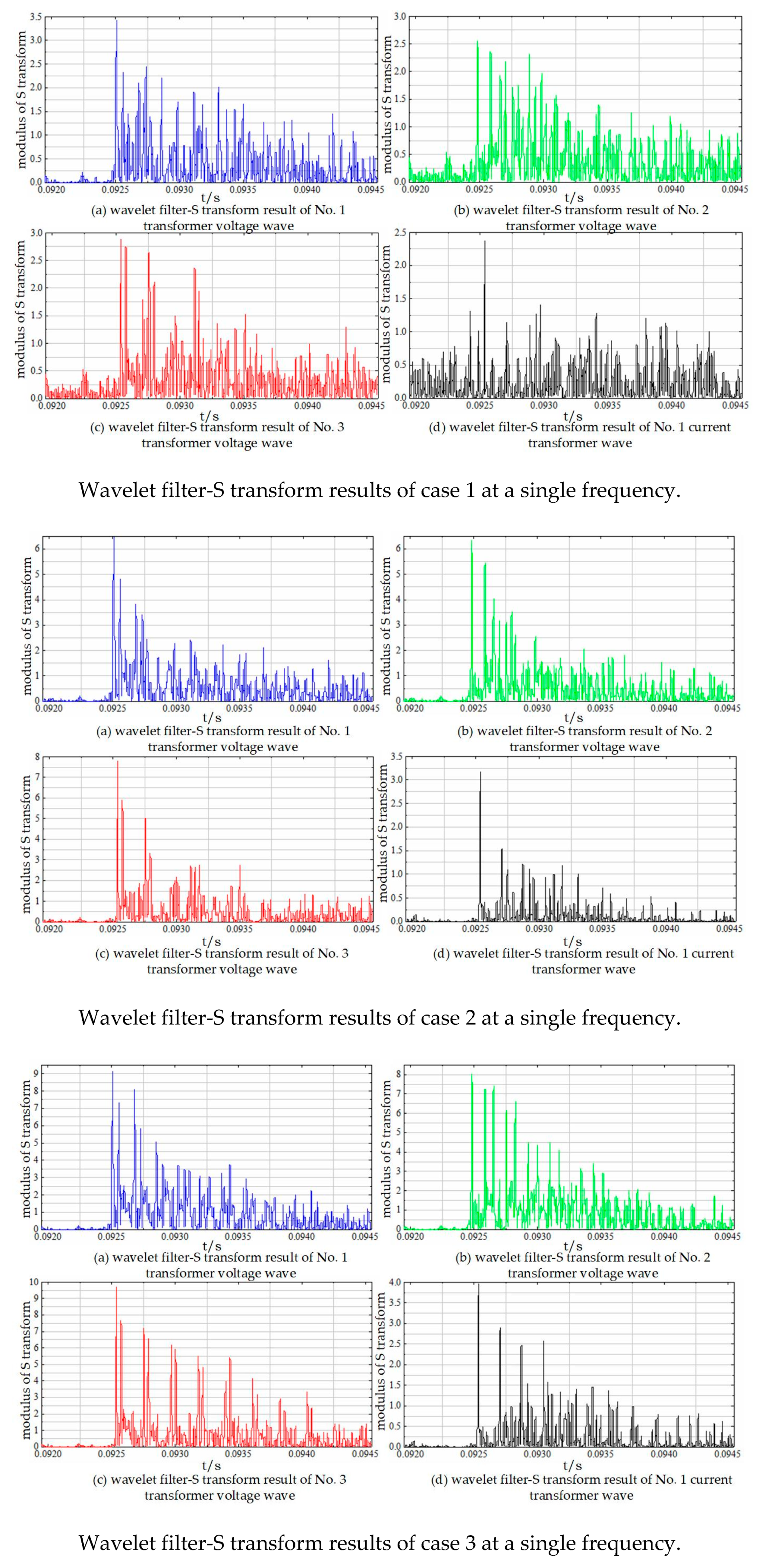
The result of the wavelet filter was used as the original data of S transform. The S modulus matrix in the range of approximately 10–100 kHz was obtained. The maximum modulus at different frequencies were defined. The corresponding moments of unique modulus maximum were used as the arrival time of the traveling wave.

(5)

The arrival time of the traveling wave was collected by each 35-KV/220 V low-voltage transformer and the line head CT. The fault location was defined based on the double-ended location principle and the distributed multi-point location model.

4. Simulation Results

In this section, the simulation model of a 35-kV high-reliability distribution network is established. The structure and simulation parameters refer to a domestic railway design in China. Three typical fault situations including single-phase grounding through transition resistance, two-phase short-circuit grounding through transition resistance, and three-phase short-circuit are simulated. The accuracy of the S-transform method, wavelet filter Hilbert–Huang transform method, and the proposed method in this article will be analyzed under the background of analog–digital conversion and noise interference.

4.1. Simulation Model and Parameters

The 35-kV high-reliability distribution networks are single power supply under normal operation. Take the continuous transmission lines as an example to build the simulation model. The simulation model is shown in Figure 7 below.

A 110-kV single unit infinite power was used to provide electricity for the model. The equivalent Thevenin voltage source model was used to simulate the power source. A 110-kV/35 kV transformer module, 35-kV/220 V transformer module, overhead transmission line module, and current and voltage measurement module were contained in the model. The unified magnetic equivalent circuit (UMEC) model and Bergeron model were used to simulate the transformer and lines. The parameter setting of each module refers to the design drawing of the domestic railway. The no-load loss of a 110-kV transformer used was 9.76 kW. The short-circuit loss was 52.5 kW. The impedance voltage was 10.5%. No-load current was 1.1%. Connection group was Ynd11. The no-load loss of the 35-kV/220 V low voltage transformer was 1.1 kW. The short-circuit loss was 6.9 kW. The impedance voltage was 6.5%. The no-load current was 2.3%. The connection group was Dyn11. The CT transformation ratio at the first of the line was 20A/5A. The rated secondary load was 0.4 Ω. The load of each low-voltage transformer was defined according to the actual transmission capacity. The end of the line was open. The type of overhead transmission line was LGJ-95. The Bergeron model was used to simulate lines. The line parameters and length are shown in

Table 2. Parameters of transmission lines.

Parameter Type of Overhead Transmission Line		Parameters of Overhead Transmission Line
Cross-sectional area/mm2	Aluminum	95.2
	Steel core	17.8
Outer radius/mm	Electric wire	13.7
	Steel core	5.4
DC resistance temperature 20 ℃/(Ω/km)		0.33
Length of Tline1 overhead transmission line/km		40
Length of Tline2 overhead transmission line/km		40
Length of Tline3 overhead transmission line/km		7
Length of Tline4 overhead transmission line/km		7
Length of Tline5 overhead transmission line/km		10
Length of Tline6 overhead transmission line/km		25
Length of Tline7 overhead transmission line/km		7

[28].

The fault is located between the No. 2 transformer and the No. 3 transformer, which was 10 km away from the No. 2 transformer. The location accuracy of the above method in different fault situations was calculated according to the fault location steps.

4.2. Result Analysis

4.2.1. Analysis of Different Fault Conditions

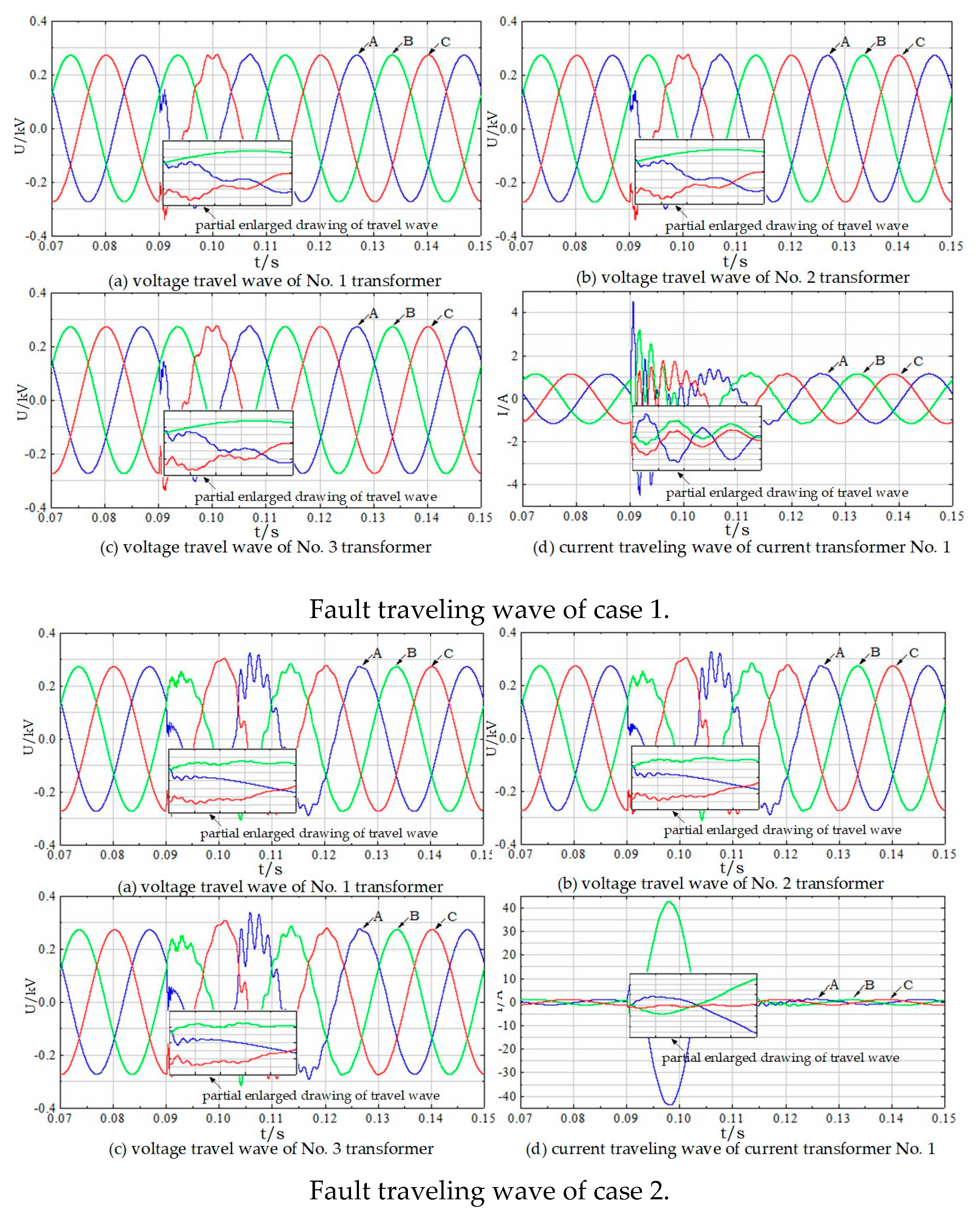
In order to fully verify the effectiveness of the proposed fault location method, three fault conditions are built in this section.

(1)

Case 1: Phase A is grounded through 100 Ω transition resistance. Single-phase grounding faults are the most frequent type of fault in the power system. The fault traveling wave characteristics are not obvious, which makes it difficult to calibrate the arrival time of the traveling wave.

(2)

Case 2: AB two-phase short circuit is grounded through 100 Ω transition resistance.

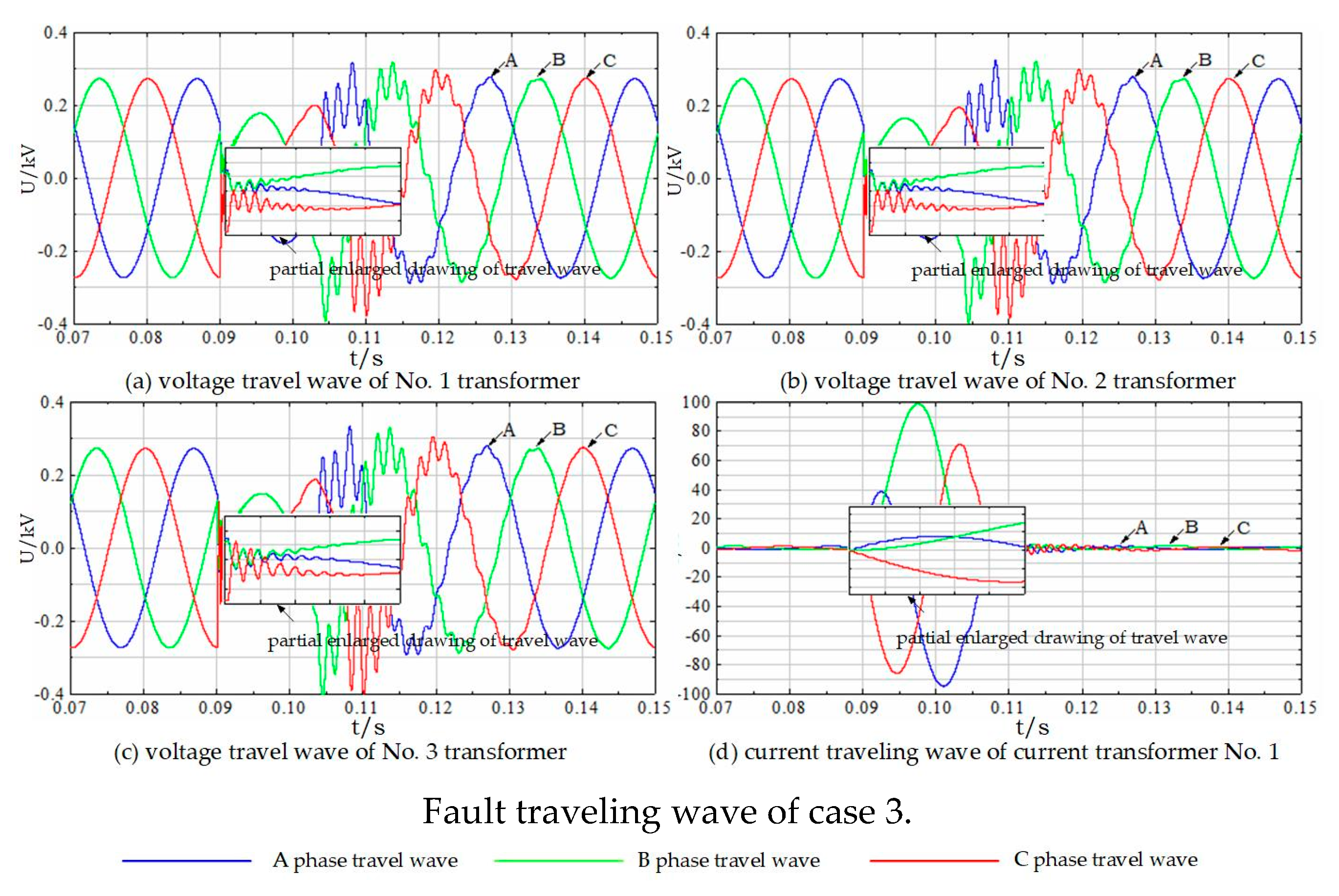
(3)

Case 3: Three-phase ABC short circuit.

The simulation time was 0.12 s. The sampling step was 0.5 μs. Fault occurrence time was 0.09245 s. The fault duration was 0.01 s. The simulation software was power systems computer-aided design. The fault traveling waves of the three situations are shown in Figure 8.

It can be seen from Figure 8 that both voltage and current had obvious traveling wave processes in the mentioned three fault conditions. The traveling wave characteristics of case 1, case 2, and case 3 are sequentially enhanced. In addition, the characteristics of the current traveling wave in each fault condition were stronger than the voltage traveling wave. The main reason was that the voltage traveling wave was collected on the secondary side of the transformer. A large number of higher harmonics cannot be transmitted to the secondary side of the transformer.

The protection of the 35-kV high-reliability distribution network had a longer response time which provided more available data. However, fault location only needed to determine the arrival time of the initial traveling wave. The selected data that can cover the initial traveling wave transmission process met the requirements. In this paper, the initial traveling wave transfer process took about 0.16 ms at most. In order to leave a time margin and subsequent expansion space, the fault location buffered a total of 4 ms data. According to the 2M sampling rate, 8000 points can be stored. The data was used for fault location. The stored 4 ms traveling wave data was simulated by analog–digital conversion based on Equations (5) and (6) and mixed with noise. Then, the line mode component of the traveling wave was obtained with the help of the Karen Bell transform. The noise and analog–digital conversion result of the fault traveling wave line mode component are shown in Figure 9.

It can be seen from Figure 9 that after the analog–digital conversion simulation and mixing noise, the singularity of the initial traveling wave was reduced. The main reason is that the analog–digital conversion reduced data accuracy. The difference between data was weakened. At the same time, high-frequency noise appeared in the fault wave, which was similar to the traveling wave caused by line faults. The fault location accuracy can be affected.

4.2.2. Comparison of Multiple Ranging Methods

In order to fully analyze the influence of noise interference and analog–digital conversion on the fault location, the effectiveness of the proposed method and the existing literature methods was verified in the above three conditions. For the convenience of description, method 1 was a single S transform method. Method 2 was a wavelet filter Hilbert–Huang Transform (HHT) method. Method 3 was the method proposed in this article.

(1)

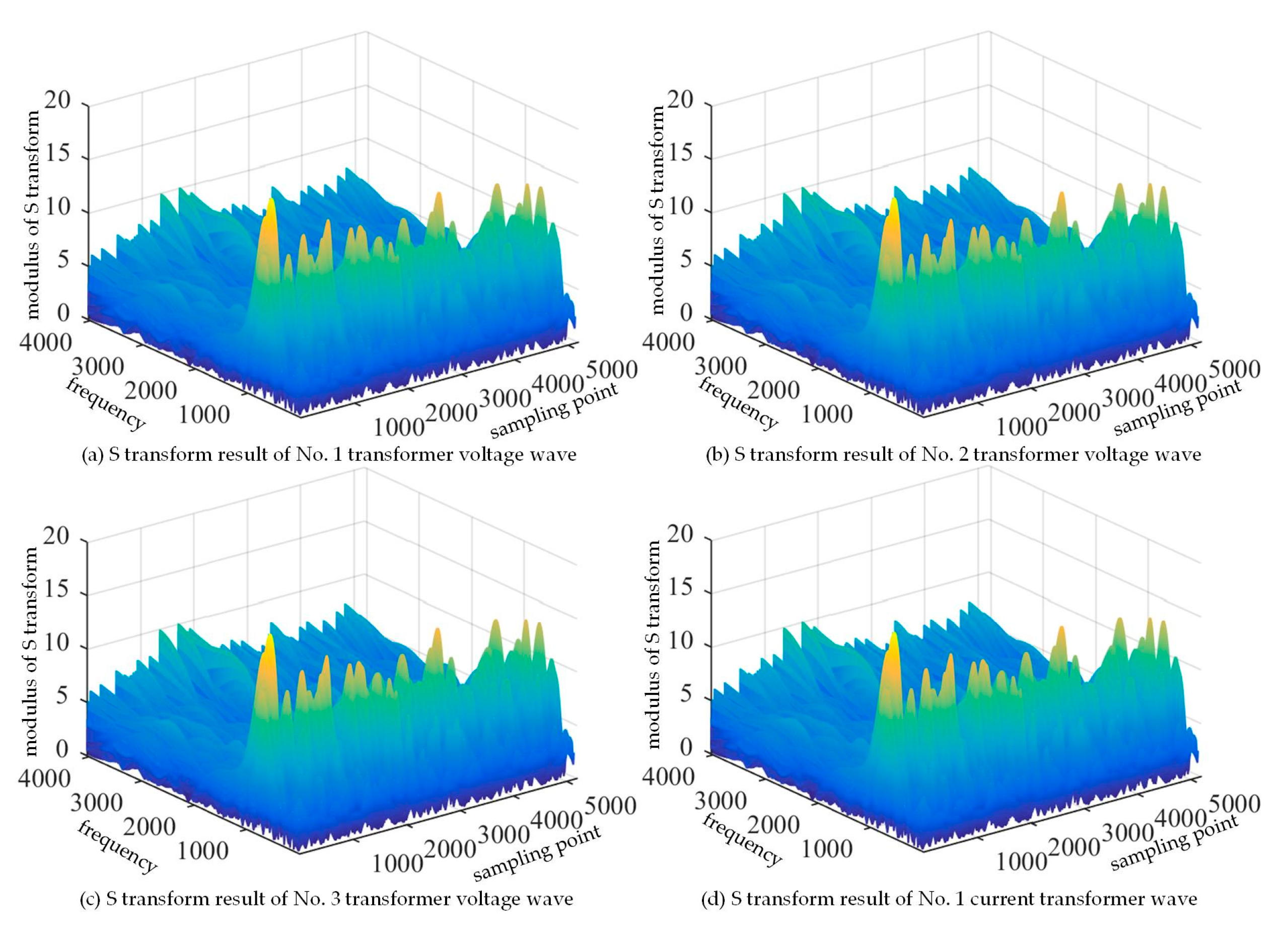
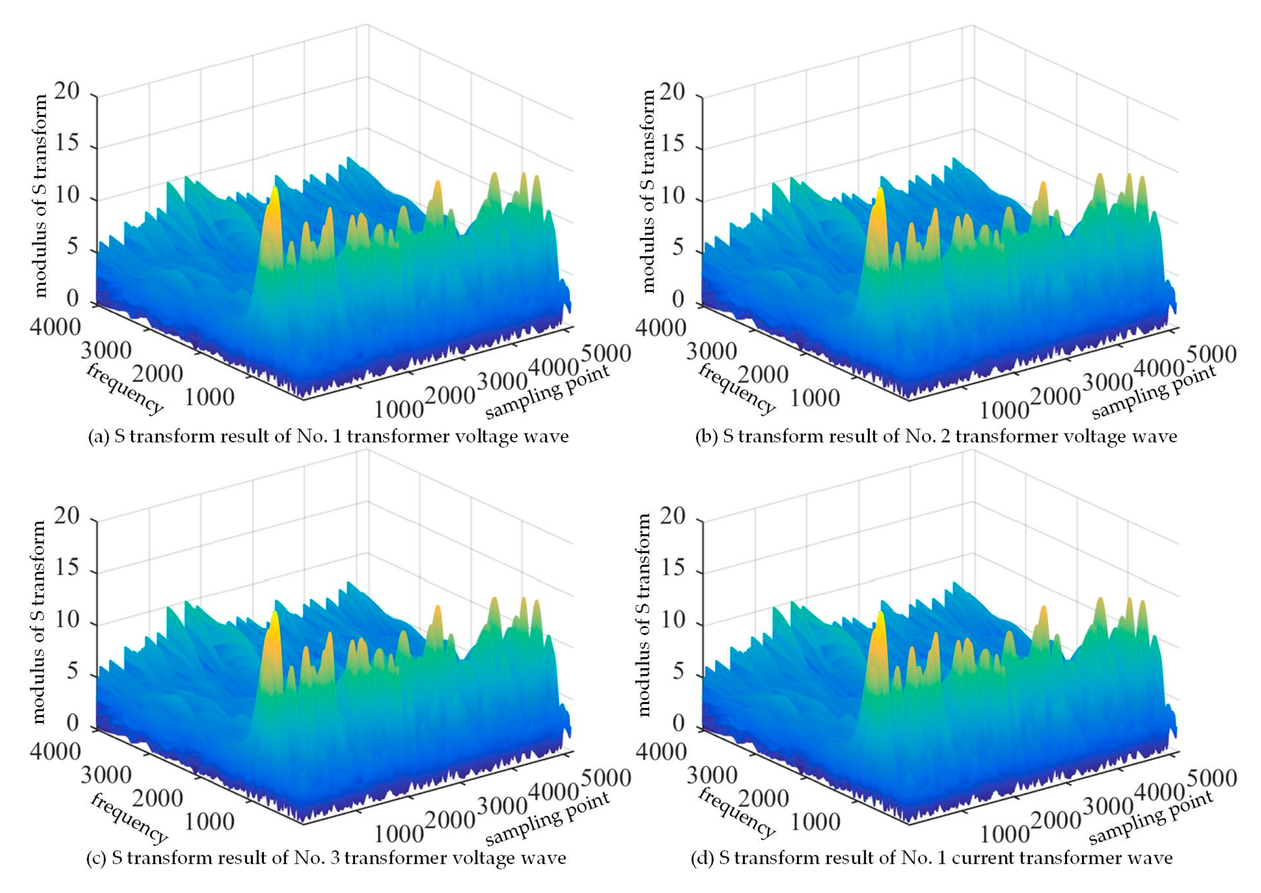
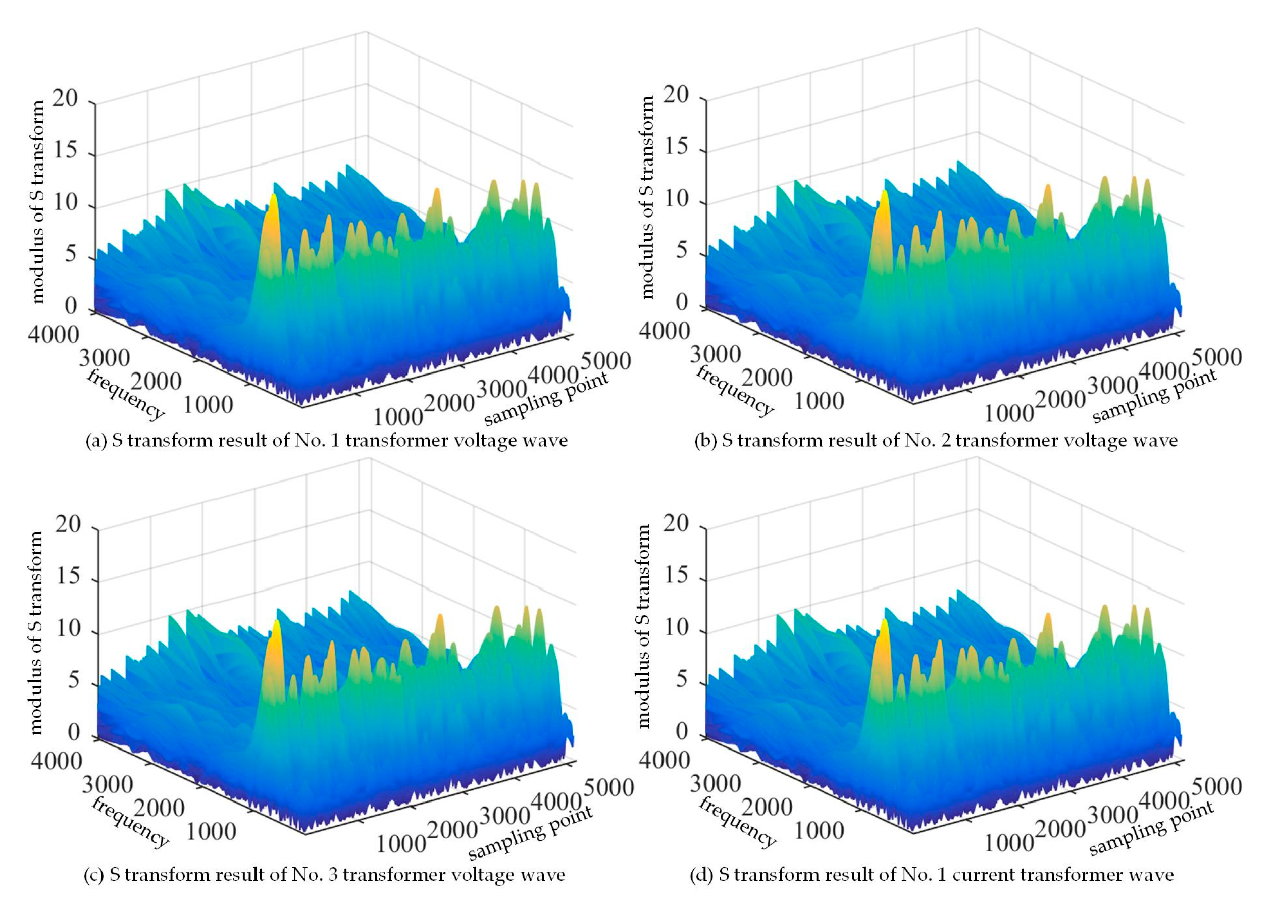
Method 1. Only S transform was used to obtain the fault traveling wave S-mode matrix. The arrival time of the traveling wave was determined according to the frequency range and the principle of modulus maximum [29]. The single S transformation results of the above three failure conditions are shown in Figure A1, Figure A2 and Figure A3 in the Appendix A. Due to the end effect, the S transform results at the head and tail were abnormally high. Therefore, the data at the head and tail were ignored in the S transform result. Only the middle part was used for arrival time calibration.

From the Figure A1, Figure A2 and Figure A3 in the Appendix A, it was seen that the maximum value of the voltage traveling wave and the current traveling wave were the same. It was impossible to distinguish the time difference of the fault travel when waves reach different sampling points. The main reason was that the analog–digital conversion weakens the singular characteristics of the fault traveling wave. The change caused by the line fault was covered by the noise signal. The modulus maximum point no longer corresponds to the arrival time of fault traveling wave. The accuracy of method 1 is shown in

Table 3. Accuracy of three methods in different conditions.

Fault Condition	Type of Method	The Fault Location is Away from the No. 2 Transformer/m		Location Error/m
		Theoretical Value	Actual Value
Condition 1	Method 1	10,000	14,033.10649	+4033.10649
	Method 2		10,948.17073	+948.170731
	Method 3		10,086.92895	+86.9289500
Condition 2	Method 1	10,000	14,033.10649	+4033.10649
	Method 2		9126.185353	−873.814647
	Method 3		10,088.52033	+88.5203300
Condition 3	Method 1	10,000	14,033.10649	+4033.10649
	Method 2		9142.498089	−857.501911
	Method 3		10,183.03030	+183.030300

under the mentioned three kinds of fault conditions.

(2)

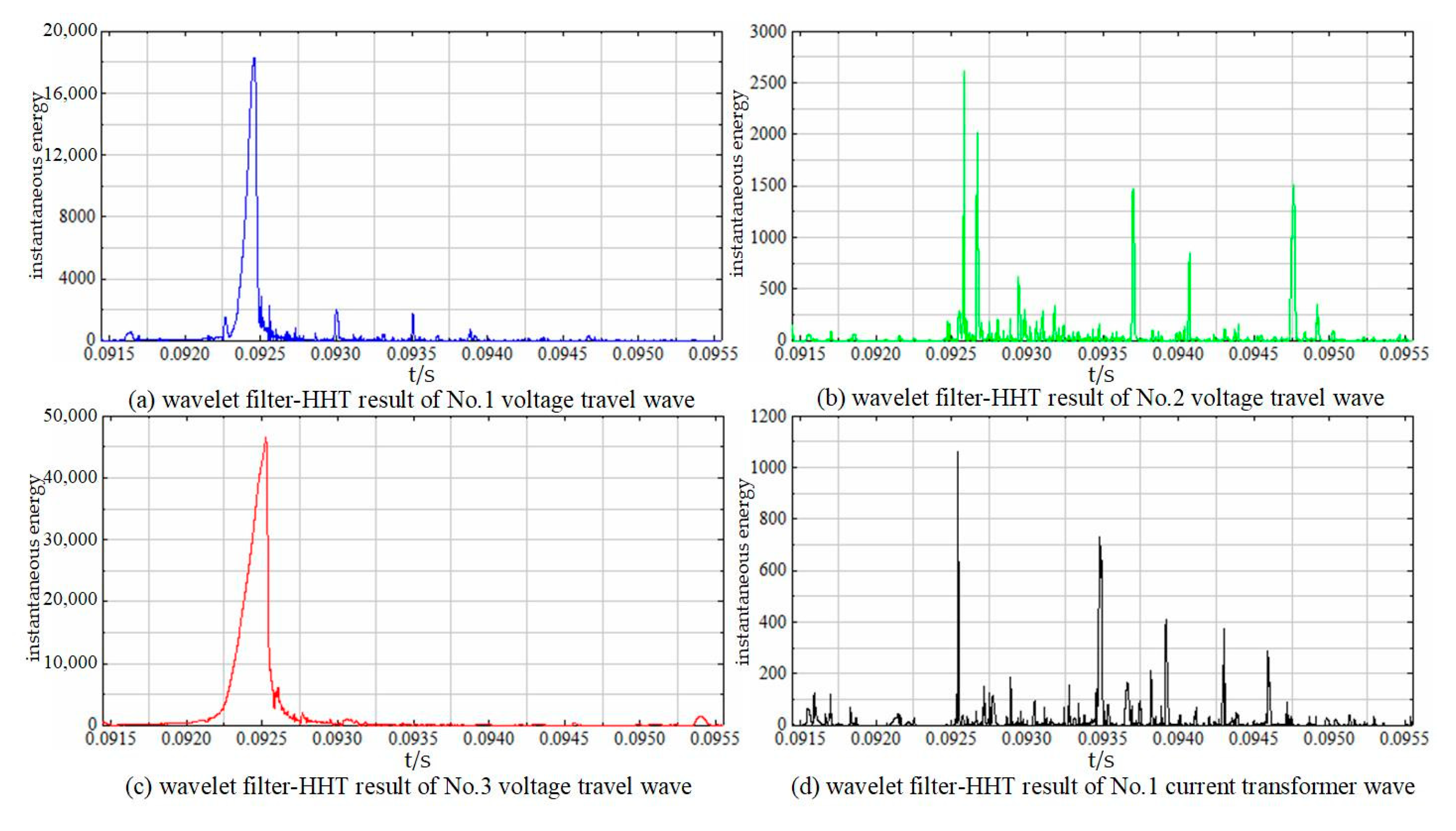
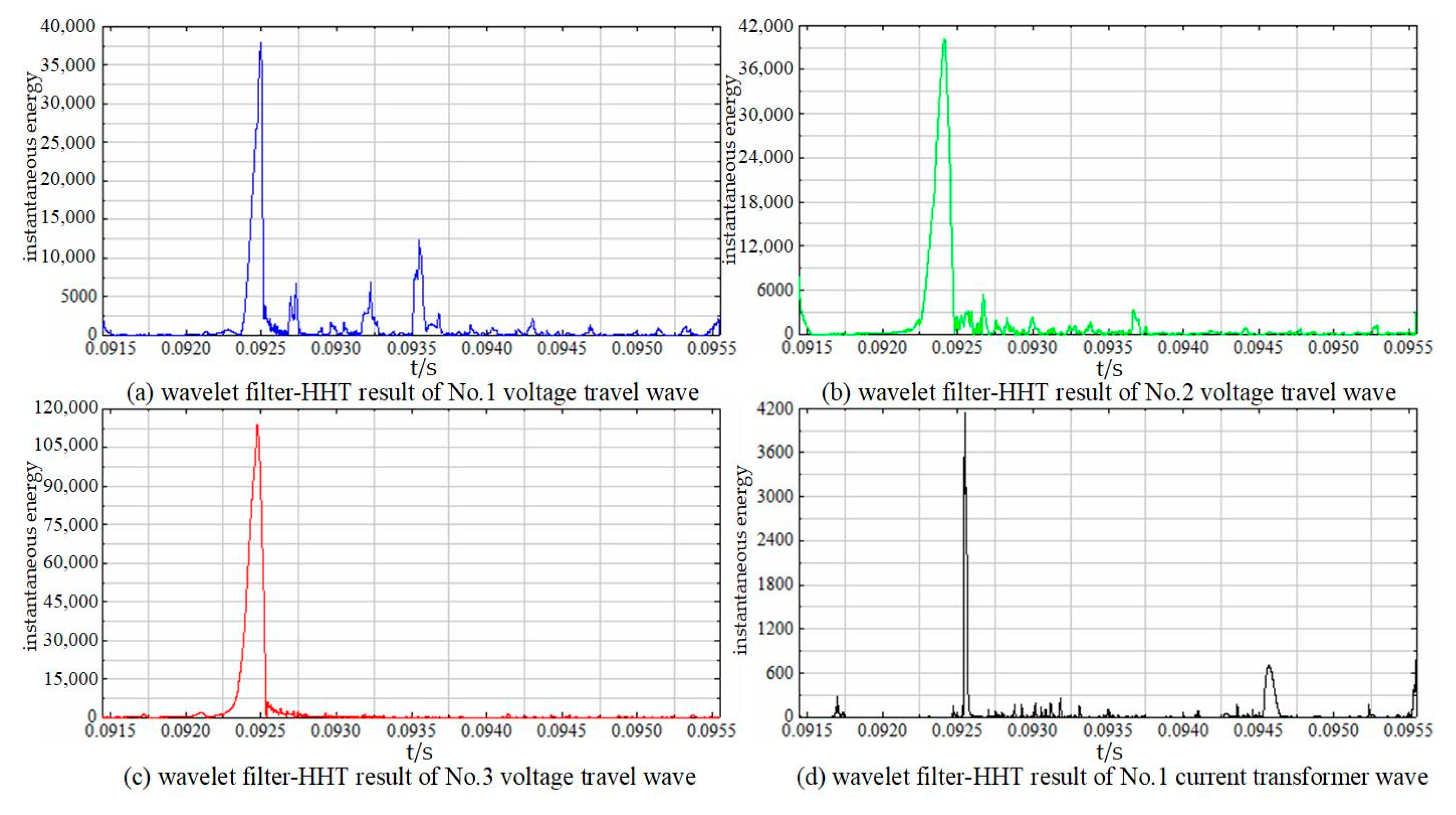
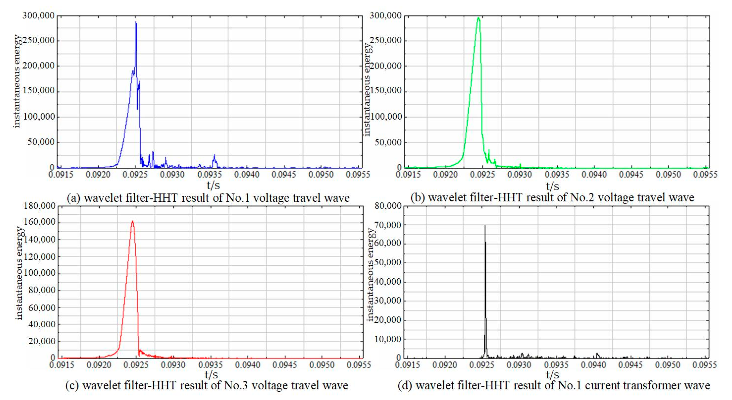
Method 2. The wavelet filter method was combined with the HHT method mentioned in the literature [7]. The data after wavelet filter was subjected to empirical mode decomposition (EMD). The high-frequency intrinsic mode function component IMF1 was used for the Hilbert–Huang Transform to obtain instantaneous energy. The maximum instantaneous energy corresponded to the arrival time of the traveling wave [7]. The HHT results of the above three fault conditions are shown in Figure A4, Figure A5 and Figure A6 in the Appendix A.

It can be seen from Figure A4, Figure A5 and Figure A6 in the Appendix A that both the voltage and current traveling waves have obvious instantaneous energy maximum. The current traveling waves were collected at the head of the line, where the instantaneous energy changes the most. The maximum instantaneous energy point corresponded to the arrival time of the traveling wave. Based on the distributed multi-point location model, the non-faulty line was used to calculate the wave speed. The location accuracy of different fault conditions is shown in Table 3.

(3)

Method 3. The method proposed in this paper was used to define the fault position of the 35-kV high-reliability distribution network. The location accuracy under different fault conditions was analyzed. The results of the method proposed in this paper are shown in Figure 10.

In Figure 10, the x-axis is the sampling point and the y-axis is the frequency. The corresponding frequency can be converted according to Equation (16). The z-axis is the S transform modulus value. It can be seen from Figure 10 that the wavelet filter-S transform results of the voltage and current traveling wave in the above fault conditions all have obvious modulus maximum points. The modulus maximum point distribution of single frequency was selected, which was also the arrival time distribution of the traveling wave. The distribution is shown in Figure 11.

In Figure 11, both the voltage and current traveling waves can distinguish obvious modulus maximum points in different conditions, which can be used to determine the arrival time of the traveling wave. For more serious faults such as a three-phase short circuit, it can also distinguish the refracted wave and the opposite reflected wave. With the help of Formula (3), the location accuracy in different conditions can be obtained, as shown in Table 3.

As can be seen from Table 3, method 1 had a higher location error in different fault conditions. The main reason was due to the influence of analog–digital conversion and noise. The modulus maximum point obtained by method 1 no longer corresponds to the arrival time of the traveling wave. The difference in the traveling wave arrival time can no longer be distinguished. Therefore, the single S transform is no longer suitable for fault location of 35-kV high-reliability distribution network under the background of noise and analog–digital conversion. Compared with Method 1, Method 2 has greater improvement in location accuracy. Although it is slightly inferior to Method 3. As the initial traveling wave of Method 2 has high instantaneous energy. The extreme points of the data are not uniformly distributed, which easily causes modal aliasing. In addition, the time-frequency information obtained by the Hilbert–Huang transform is not rich enough compared with the S transform. In Method 3, the more elaborate time–frequency information of the S transform is obtained, which greatly improves the location accuracy of the above three fault situations. The result can provide the fault location reference for the 35-kV high-reliability distribution network inspection.

In the experiment, the real operating environment of the distribution network is more complicated. There are more interference signals, such as extreme weather. Earth’s capacitance is changed with different weather and sag. Higher earth capacitance makes the features of fault traveling wave less obvious. The actual load of different transformers is not constant. Low loads make the features of the traveling wave collected from the secondary side of the transformer non-obvious enough. The differences between the experiment and simulation affect the determination of the traveling wave arrival time and make the fault location accuracy of the experiment lower than the results proposed in this paper.

At present, some literature has partly verified the application of traveling wave fault location. Design of the manual grounding experiment of the distribution network was as in the literature [19]. The traveling wave transmission performance of the distribution transformer has been verified. The experimental results show that distribution transformers can effectively transmit traveling waves. The accuracy of transmission can meet the fault location requirements. The traveling wave transmission features of distribution transformers are related to the neutral grounding of the transformer windings. Literature [30] uses the fault data recorded on a distribution station to verify the effectiveness of traveling wave transmission features of the current transformer. The results reflect that current transformers can transfer the characteristics of the traveling wave, which meet the requirements of fault location. These literature show that the fault location method proposed in this paper has feasibility in practice. The improvements are marked in red in the last paragraph of Section 4.2.2.

5. Conclusions

Based on the power supply structure of a 35-kV high-reliability distribution network, the current and the travel voltage along the line is comprehensively used for the distributed multi-point location model in this paper. The fault location method of wavelet filter-S transformation is proposed considering the influence of analog–digital conversion and noise signal on the fault location accuracy. The effectiveness of the proposed method is verified by the simulation example. The conclusions are as follows.

(1)

Wave speed is calculated based on the actual travel time in a multi-point location model. The method avoids that the traditional calculation method of wave speed only considers the line parameters and fails to analyze the influence of the environment on the wave speed. The location error caused by inaccurate wave speed is reduced.

(2)

Analog–digital conversion and noise will weaken the singular characteristics of the line fault traveling wave. The change caused by the line fault might be covered by the noise signal. The single S transform modulus maximum method cannot be used to locate the fault. The method proposed in this paper can effectively reduce the influence of noise on the identification of the traveling wave.

(3)

The simulation results show that the method proposed in this paper has high location accuracy under the conditions of single-phase grounding through transition resistance, two-phase short-circuit grounding through transition resistance, and three-phase short-circuit.

References

1. State Development and Reform Commission. Action Plan for Construction and Transformation of Distribution Network (2015–2020); The State Development and Reform Commission: Beijing, China, 2017.
2. Hong, Y.; Tan, Y.H.; Yi, H.L. New method of single phase-to-ground fault location based on traveling wave in distribution networks. Proc. CSU-EPSA 2017, 29, 14–20. [Google Scholar]
3. Hu, M.; Chen, H. Detection and location of power quality disturbances using wavelet transform modulus maxima. Power Syst. Technol. 2001, 25, 12–16. [Google Scholar]
4. Han, Z.; Li, S.; Liu, S.; Gao, S. Generalized Fault-Location Scheme for All-Parallel AT Electric Railway System. Energies 2020, 13, 4081. [Google Scholar] [CrossRef]
5. Ji, Y.Y.; He, J.H. Application of travelling wave based fault location in 10kV railway automatic blocking and continuous power transmission lines. Power Syst. Technol. 2003, 27, 13–15. [Google Scholar]
6. Deng, F.; Li, X.R.; Zeng, X.J. Single-ended traveling-wave-based fault location algorithm for hybrid transmission line based on the full-waveform. Trans. China Electrotech. Soc. 2018, 33, 3471–3482. [Google Scholar]
7. Xiong, L.B.; Wu, G.H.; Wang, Z.X. Study on fault location of multi measuring points traveling wave method based on IHHT in all parallel AT traction network. Trans. China Electrotech. Soc. 2019, 35, 3244–3252. [Google Scholar]
8. Li, Z.B.; Xu, Y.H.; Wu, B.X. Fault location of high voltage transmission line based on S-transform traveling wave method. Electr. Meas. Instrum. 2014, 51, 40–42. [Google Scholar]
9. Qian, J.Q.; Ye, J.Z.; Kuang, Z. A fault location method for multi-terminal transmission network based on S transform. Power Syst. Prot. Control 2014, 42, 82–88. [Google Scholar]
10. Xie, L.W.; Liu, Y.X.; Zeng, X.J. Fault Location of Multi-terminal Transmission Lines Based on VMD and S Transform. Proc. CSU-EPSA 2019, 31, 126–134. [Google Scholar]
11. Dai, F.; Ye, Y.Y.; Liu, Z.Y. Research on fault location of transmission line based on S-transform and synchronized phasor measurement. Electr. Meas. Instrum. 2020, 57, 13–19, 44. [Google Scholar]
12. Pang, Z.J.; Du, J.; Jiang, F.; He, L.; Li, Y.; Qin, L.; Li, Y. A Fault Section Location Method Based on energy Remainder of Generalized S-Transform for Single-phase round Fault of Distribution Networks. In Proceedings of the IEEE Advanced Information Technology, Electronic & Automation Control Conference, Chongqing, China, 12–14 October 2018; pp. 1511–1515. [Google Scholar]
13. Wu, Y.Y.; Shu, Q. Algorithm research of S transform in the analysis of fault traveling wave signal in distribution network. Digit. Technol. Appl. 2017, 4, 135–137, 141. [Google Scholar]
14. Liu, X.L. Research on common faults and preventive measures of urban distribution network lines. Commun. World 2017, 21, 266–267. [Google Scholar]
15. Guo, H.Q. Study on Fault Locating of 10 kV Automatic Blocking and Continuous Transmission Lines of Railway Based on Traveling Wave Method. Master’s Thesis, Shijiazhuang Tiedao University, Shijiazhuang, China, 2019. [Google Scholar]
16. Nduwamungu, A.; Ntagwirumugara, E.; Mulolani, F.; Bashir, W. Fault Ride through Capability Analysis (FRT) in Wind Power Plants with Doubly Fed Induction Generators for Smart Grid Technologies. Energies 2020, 13, 4260. [Google Scholar] [CrossRef]
17. Liu, X.Q.; Wang, D.Z.; Jiang, X.C. Fault location algorithm for distribution power network based on relationship in time difference of arrival of traveling wave. Proc. CSEE 2017, 37, 4109–4115. (In Chinese) [Google Scholar]
18. Zhao, J.X.; Li, J.H.; Chang, Q. Study on GPS timing and frequency calibration method and the test results. J. Beijing Univ. Aeronaut. Astronaut. 2004, 8, 762–766. [Google Scholar]
19. Ji, T.; Sun, T.J.; Xu, B.G. Traveling waves measurement with distribution transformers. Autom. Electr. Power Syst. 2006, 16, 66–71. [Google Scholar]
20. Zhu, Y.L.; Fan, X.Q.; Yin, J.L. A new fault location scheme for transmission lines based on traveling waves of three measurements. Trans. China Electrotech. Soc. 2012, 27, 260–268. [Google Scholar]
21. Wang, Q.J.; Jin, T.; Shen, T. A complete analytic model of section location in distribution network based on multi-factor dimensionality deduction. Trans. China Electrotech. Soc. 2019, 34, 3012–3024. [Google Scholar]
22. Yu, H.N.; Ma, C.C.; Wang, H. Research on transmission line fault location method based on compressed sensing estimating traveling wave natural frequency. Trans. China Electrotech. Soc. 2017, 32, 140–148. [Google Scholar]
23. Pan, Q.; Meng, J.L.; Zhang, L. Wavelet filtering method and its application. J. Electron. Inf. Technol. 2007, 29, 236–242. [Google Scholar]
24. Donoho, D.L. De-Noising by Soft-Thresholding. IEEE Trans. Signal Process. 1995, 41, 613–627. [Google Scholar] [CrossRef] [Green Version]
25. Stockwell, R.G.; Mansinha, L.; Lowe, R.P. Localization of the complex spectrum: The S transform. IEEE Trans. Signal Process. 1996, 44, 998–1001. [Google Scholar] [CrossRef]
26. Liu, Q.; Tai, N.L.; Fan, C.J. Phase-mode transformation of asymmetry-parameter four-parallel lines on the same tower. Trans. China Electrotech. Soc. 2015, 30, 171–1803. [Google Scholar]
27. Xu, M.M.; Xiao, L.Y.; Lin, L.Z. Single phase ground fault location method for distribution lines based on zero-mode traveling wave attenuation characteristics. Trans. China Electrotech. Soc. 2015, 30, 397–404. [Google Scholar]
28. Northwest Electric Power Design Institute. Power Engineering Design Manual Volume 3; Shanghai People’s Publishing House: Shanghai, China, 2010. [Google Scholar]
29. Brown, R.A.; Lauzon, M.L.; Frayne, R. A General Description of Linear Time-Frequency Transforms and Formulation of a Fast, Invertible Transform That Samples the Continuous S-Transform Spectrum Nonredundantly. IEEE Trans. Signal Process. 2010, 58, 281–290. [Google Scholar] [CrossRef]
30. Ji, T.T. Study on Fault Location of Distribution Network Feeders Based on Transient Traveling Waves; Shandong University: Shandong, China, 2015. [Google Scholar]
Figure 1. Diagram of automatic blocking and continuous transmission lines.
Energies 13 05118 g001
Figure 2. Principle of two-terminal fault location.
Energies 13 05118 g002
Figure 3. Diagram of continuous transmission lines.
Energies 13 05118 g003
Figure 4. Traveling waves of voltage and current at different points.
Energies 13 05118 g004
Figure 5. Result of noise sampling.
Energies 13 05118 g005
Figure 6. Distribution of noise frequency.
Energies 13 05118 g006
Figure 7. Model of simulation.
Energies 13 05118 g007
Figure 8. Waves of current and voltage in different conditions.
Energies 13 05118 g008aEnergies 13 05118 g008b
Figure 9. Line mode component noise and AD simulation result in different conditions.
Energies 13 05118 g009aEnergies 13 05118 g009b
Figure 10. Wavelet filter-S transform results in different conditions.
Energies 13 05118 g010aEnergies 13 05118 g010b
Figure 11. Wavelet filter-S transform results of single frequency in different conditions.
Energies 13 05118 g011