Variable Bandwidth Adaptive Course Keeping Control Strategy for Unmanned Surface Vehicle

Abstract

This paper proposes a new and original course keeping control strategy for an unmanned surface vehicle in the presence of modeling error, external disturbance and input saturation. The trajectory linearization control method is used as the basic algorithm to design the course keeping strategy, and the radial basis function neural network and disturbance observer are used to compensate modeling error and external disturbance respectively to enhance the robustness of the control system. Moreover, a robust term is used to compensate various compensation errors to further improve the robustness of the system. In addition, hyperbolic tangent function and Nussbaum function are hired to deal with the potential input saturation problem, and the neural shunting model is adopted to avoid the computational explosion caused by the derivation of virtual control law. Taking the above facts into account will help to further realize engineering practice. Finally, the control strategy proposed in this paper is compared with the classical proportional–integral–derivative control strategy. The simulation results show that the course control results of the proposed control strategy are more robust than proportional–integral–derivative control, regardless of whether the external disturbance is weak or strong.

1. Introduction

An unmanned surface vehicle (USV) is a small surface sports platform that can carry multiple functional modules and accomplish specific missions, and it is called the Unmanned Three Musketeers (UTM) together with unmanned vehicle and unmanned aerial vehicle (UAV) [1,2,3,4,5,6]. Due to the fact that modern combat methods have undergone tremendous changes, how to protect the personal safety of soldiers and minimize casualties has become a top priority. It can be said that the development of unmanned combat platforms is an inevitable measure to adapt to historical development trends. Therefore, as an important part of the unmanned combat platforms at sea, the USV is gradually receiving great attention from research institutions from all over the world, especially military powers. The essential reason why USV has various advantages is that it can navigate independently. In other words, it is equipped with an autonomous navigation system, in which course keeping control is the most basic function of the autonomous navigation control system. Course keeping control can ensure that the USV travels in a fixed course to achieve the goal of safety and energy saving [7,8].

Scholars have made a large number of outstanding contributions to ship course control. The first generation of ship course autopilot was invented by Elmer Sperry, which uses a gyrocompass to measure course angle. Another important breakthrough is that the proportional–integral–derivative (PID) control algorithm is proposed and applied to the autopilot [9]. To cope with these issues, backstepping technology [10,11], sliding mode control [12,13], adaptive technology [14] and linear quadratic Gaussian [15], etc., are hired to design control solutions. In [16], under the premise that the model parameters are unknown, an adaptive course controller is designed by backstepping method and adaptive technique. At the same time, an integral term is introduced into the control law to eliminate static errors. In the design process of designing the ship’s course controller, all uncertainties, including internal uncertainties and external disturbances, are considered as a whole and compensated by disturbance observer (DOB) [17]. Kahveci et al. propose a course control law for uncertain ship dynamics subject to input constraints under changing external disturbance [18]. Peng et al. present an autopilot design for a robotic unmanned surface vehicle in the presence of unknown yaw dynamics and measurement noises. Meanwhile, numerical simulation and field experiment are performed to verify the correctness of the control strategy [19]. Zhang et al. propose a nonlinear feedback strategy with strong robustness [20]. Based on [20,21], an improved feedback control law which is more suitable for small USV is proposed. In [22], a fast convergent course control strategy is proposed by combining a linear sliding mode with a non-singular terminal sliding mode. In engineering practice, the universal approximation ability of the radial basis function (RBF) neural network and fuzzy logic is most often employed to estimate unknown functions in the model. In addition, the problem of input saturation needs to be taken into account. If it is not taken into account, it is possible that the computational output of the controller is greater than the maximum that the actuator can provide. In [23], an aided design system is designed to analyze potential input saturation problems in the system.

Motivated by the above analysis, a novel variable bandwidth adaptive course keeping strategy, which is designed by using the trajectory linearization control (TLC) method, RBF neural network, disturbance observer, adaptive technology, neural shunting model, hyperbolic tangent function and Nussbaum function, is developed for an USV with modeling error and external disturbance. The main innovations of this paper are as follows:

(1) From the author’s point of view, the novel variable bandwidth control has been applied to the course control of USV for the first time. In the process of controller design, many practical situations are taken into account, such as modeling error, external disturbance and input saturation. The TLC method is introduced into the course keeping strategy, and the robustness of the controlled system is improved by using RBF neural network, disturbance observer, adaptive technology. The TLC method itself is a simple and effective control method and convenient for engineering application, which is also introduced into the design of ship motion controller by our team.

(2) Hyperbolic tangent function is hired to solve the input saturation issue. Meanwhile, introducing Nussbaum function simplifies the problem that control strategies are difficult to design due to input saturation.

(3) In order to be more practical and convenient for engineering application, neural shunting model is adopted to reduce the computational burden of the controller. The above considerations lay the foundation for the application of the control strategy proposed in this paper to the real ship control in the next step.

The rest of this note is organized as follows. Section 2 states problem formulation and preliminaries. Section 3 presents the design process of the control scheme. Section 4 verifies the stability of the system. In Section 5, the simulations are carried out to prove the correctness and robustness of the control strategy. Section 6 concludes this paper.

2. Problem Formulation and Preliminaries

2.1. Problem Formulation

The non-linear response model, namely Norrbin model, is used to describe the relationship between course and rudder angle [24].

Define $x={\left[\begin{array}{cc}{x}_1& x_2\end{array}\right]}^T$, $f(x)={\left[\begin{array}{cc}{x}_2& -\frac{1}{T}{x}_2-\frac{\alpha }{T}{x}_2^3\end{array}\right]}^T$, $g_1(x)={\left[\begin{array}{cc}0& \frac{K}{T}\end{array}\right]}^T$, $g_2(x)={\left[\begin{array}{cc}0& 1\end{array}\right]}^T$, $g_3(x)={\left[\begin{array}{cc}0& \Delta \end{array}\right]}^T$, and then the nonlinear response model can be expressed as

$$\begin{array}{c}\hfill \left\{\begin{array}{c} \dot{x}=f(x)+g_3(x)f(x)+g_1(x)u+g_2(x)d\hfill \\ y=x_1\hfill \end{array}\right.\end{array}$$

(1)

where x stands for system variable, $x_1$ is the USV’s course, $x_2$ is the yaw rate, K, T and $\alpha$ represent model coefficients, $\Delta$ is hired to describe the degree of modeling error, u represents the rudder angle, $-{35}^{\circ }\le u\le {35}^{\circ }$, and d indicates slow time-varying external disturbance.

Control objective: The control objective is to develop an adaptive course keeping control strategy to settle the above adverse factors, such that the course of USV can be closely followed and maintained at the target value ${\overline{x}}_1$.

Assumption1. 

Assume that Δ and d satisfy $\left|\Delta \right|\le \overline{\Delta }$ and $\left|d\right|\le \overline{d}$, where $\overline{\Delta }$ and $\overline{d}$ denote unknown normal numbers.

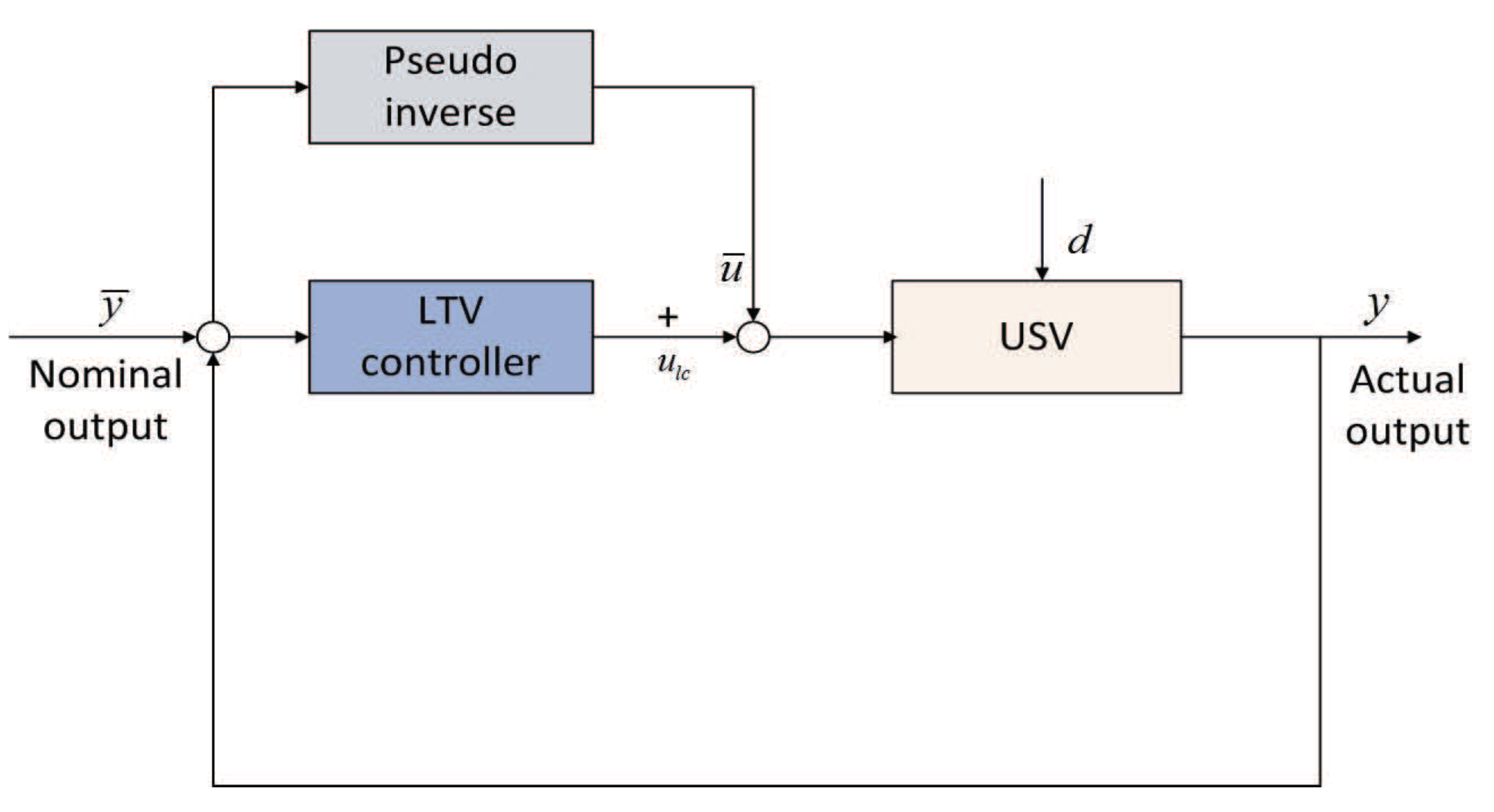
2.2. Trajectory Linearization Control

The TLC method is a novel and effective non-linear tracking and decoupling control scheme emerging in recent years [25]. At present, it has been successfully applied to control systems such as robots and aircraft [26,27]. Among the control problems, the goal of most designs is to hope that the state or output of the controlled object tracks the desired nominal instruction under the action of the corresponding control law. The TLC method uses an open-loop controller to cancel out the nonlinear part of the controlled object, which makes it more agile to the response and can reduce the trajectory tracking error caused by the linearization of the model. The design idea is that the problem of trajectory tracking is transformed into a problem of tracking error adjustment by using the non-linear dynamic inverse method, and then the feedback control law is designed by using the $PD$ spectrum theory of linear time-varying system to make the error tracking system stable.

The single input single output nonlinear system is described as follows:

$$\begin{array}{c}\hfill \left\{\begin{array}{c} \dot{x}=m(x)+m_1(x)u+m_2(x)d\hfill \\ y=h(x)\hfill \end{array}\right.\end{array}$$

(2)

where $x\in R^n$, $u\in R$, $y\in R$ are system state, control input and output, respectively, $d\in R^n$ can be viewed as a sum of factors such as system modeling error, unknown dynamics and external disturbance, $m(x)$, $m_1(x)$, $m_2(x)$ and $h(x)$ are smooth bounded functions. $m_3(x)$ and $m_2(x)$ satisfy the matching condition. That is, there is a reversible nonlinear function matrix $m_1(x)$, so that $m_1(x)m_3(x)=m_2(x)$ is established.

Define $d=0$ and according to the TLC design method [28,29], the nominal model can be expressed as

$$\begin{array}{c}\hfill \left\{\begin{array}{c} \dot{\overline{x}}=m(\overline{x})+m_1(\overline{x})\overline{u}\hfill \\ \overline{y}=h(\overline{x})\hfill \end{array}\right.\end{array}$$

(3)

where $\overline{x}\in R^n$, $\overline{u}\in R$, $\overline{y}\in R$ are the nominal state, nominal input and nominal output of the system respectively. The meaning of $m(\overline{x})$, $m_1(\overline{x})$ and $h(\overline{x})$ is the same as those in (2).

The tracking error $e_0=x-\overline{x}$ is defined, and the control law is selected to be $u=\overline{u}+u_{lc}$. Based on this, tracking error can be simplified as (4).

$$\begin{array}{cc}\hfill {\dot{e}}_0& =m(\overline{x}+e_0)+m_1(\overline{x}+e_0)(\overline{u}+u_{lc})-m(\overline{x})-m_1(\overline{x})\overline{u}\hfill \\ \hfill & =M(\overline{x},\overline{u},e_0,u_{lc})\hfill \end{array}$$

(4)

At this point, the tracking problem of the original nonlinear system is transformed into a non-linear regulation problem. That is, the control law consists of two parts: (1) for the open-loop controlled object, a nominal control input $\overline{u}$ is generated according to the desired system output $\overline{y}$; (2) the closed-loop state feedback regulator $u_{lc}$ is used to stabilize the controlled system and make it have certain response characteristics.

The frame structure of TLC technology is shown in Figure 1.

$\overline{x}$ and $\overline{u}$ can be considered as nonlinear parameters of the system, and (4) can be rewritten as ${\dot{e}}_0=M(t,e_0)$. Consider the following linear time-varying system.

$$\begin{array}{c}\hfill {\dot{e}}_0=A(t)e_0+B(t)u_{\mathrm{lc}}\end{array}$$

(5)

where $A(t)=(\frac{\partial m}{\partial x}+\frac{\partial m_1}{\partial x}u)\left|{}_{\overline{x},\overline{u}}\right.$ and $B(t)=m_1\left|{}_{\overline{x},\overline{u}}\right.$.

Assumption2. 

$A(t)$ and $B(t)$ are completely controllable.

Assumption3. 

$e_0=0$ is an isolated equilibrium point of ${\dot{e}}_0=M(t,e_0)$. $M:[0,\infty )\times D_e\to {\mathsf{\Re }}^n$ and $D_e=\{e_0\in {\mathsf{\Re }}^n∥e_0∥<\upsilon \}$ is continuously differentiable.

Based on the Assumptions 2 and 3, and TLC theory [27], the linear time-varying feedback control law can be designed as

$$\begin{array}{c}\hfill u_{lc}=K(t)e_0(t)\end{array}$$

(6)

$u_{lc}$ makes the linear time varying system (5) exponentially stable at equilibrium points and can be recorded as

$$\begin{array}{c}\hfill A_C(t)=A(t)+B(t)K(t)\end{array}$$

(7)

According to Theorem 4.13 in [11], $u_{lc}$ can guarantee that ${\dot{e}}_0=M(t,e_0)$ is exponentially stable at $e_0=0$. The specific design methods of $\overline{u}$ and $u_{lc}$ can be referred to the papers [28,29,30]. Then define the following Lyapunov function candidate.

$$\begin{array}{c}\hfill A_C^T(t)P(t)+P(t)A_c(t)+\dot{P}(t)+Q(t)=0\end{array}$$

(8)

where $P(t)$ is the positive symmetrical solution of Lyapunov equation, $Q(t)$ is a positive symmetrical matrix. $P(t)$ and $Q(t)$ meet the following conditions: $0<{\alpha }_{1}I\le P(t)\le {\alpha }_{2}I,\forall t\ge t_0$, ${\alpha }_1,{\alpha }_2>0$, $0<{\beta }_{1}I\le Q(t)\le {\beta }_{2}I,\forall t\ge t_0$, ${\beta }_1,{\beta }_2>0$.

However, in practical engineering, the factors such as unmodeled dynamics and external disturbances can not be ignored. In other words, d is not zero. In this case, the tracking error can be re represented as

$$\begin{array}{c}\hfill {\dot{e}}_0=F(t,e_0)+m_2(x)d\end{array}$$

(9)

When $∥d∥$ is small, the TLC method shows good robustness to both regular and singular disturbances. Nevertheless, if $∥d∥$ is large enough to exceed the control range of TLC, the final control performance will be unsatisfactory, and even lead to system crash.

2.3. Neural Shunting Model

In 1988, Grossberg proposed a neural shunting model to describe the individual’s real-time adaptation to the external environment [31]. It has been widely used in the fields of machine vision, robot path planning, and robot arm trajectory generation [32]. Neural shunting model can be described as

$$\begin{array}{c}\hfill {\dot{\beta }}_u=-A{\beta }_u+(B-{\beta }_u)f({\alpha }_u)-(D+{\beta }_u)g({\alpha }_u)\end{array}$$

(10)

where ${\beta }_u$ stands for the action point of the neuron, A, B and D represent positive parameters to be designed, $f({\alpha }_u)$ is the external excitation signal and $g({\alpha }_u)$ represents the external suppression signal. $f({\alpha }_u)$ and $g({\alpha }_u)$ are threshold functions, which are defined as $f({\alpha }_u)=max\left\{{\alpha }_u,0\right\}$ and $g({\alpha }_u)=max\left\{-{\alpha }_u,0\right\}$. They can be specifically described as $f({\alpha }_u)=\left\{\begin{array}{c}{\alpha }_u,{\alpha }_u\ge 0\hfill \\ 0,{\alpha }_u<0\hfill \end{array}\right.$ and $g({\alpha }_u)=\left\{\begin{array}{c}0,{\alpha }_u>0\hfill \\ -{\alpha }_u,{\alpha }_u\le 0\hfill \end{array}\right.$.

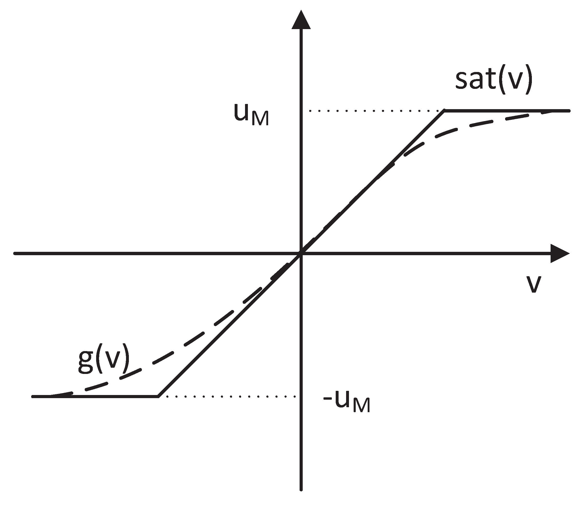
2.4. Input Saturation

Considering the physical limitations in engineering practice, there is input saturation in the controlled system. The input saturation problem can be described as (11).

$$\begin{array}{c}\hfill u=sat(v)=\left\{\begin{array}{c} \mathrm{sgn}(v)u_M,\left|v\right|\ge u_M\hfill \\ v,\left|v\right|<u_M\hfill \end{array}\right.\end{array}$$

(11)

where v is the commanded control value calculated by control law, $u_M$ is the limiting amplitude of v, u is the ultimate control input. Clearly, the relationship between the commanded control value v and the ultimate control input u has a sharp corner when $\left|v\right|=u_M$.

The saturation function can be approximated by the following hyperbolic tangent function [33].

$$g(v)=u_M\times tanh(\raisebox{1ex}{$v$}\!\left/ \!\raisebox{-1ex}{$u$}\right.)=u_M\frac{e^{v/u_M}-e^{-v/u_M}}{e^{v/u_M}+e^{-v/u_M}}$$

(12)

The principle of input saturation is shown in Figure 2.

Define $d_1(v)$ as the approximation error, which can be expressed as $d_1(v)=sat(v)-g(v)$. As can be seen from Figure 2, $d_1(v)$ belongs to a bounded function and its bound is

$$\begin{array}{c}\hfill \left|d_1(v)\right|=\left|sat(v)-g(v)\right|\le u_M(1-tanh(1))=E\end{array}$$

(13)

Easy to verify, when $\left|v\right|\le u_M$, as $\left|v\right|$ increases from 0 to $u_M$, $\left|d_1(v)\right|$ increases from 0 to E; when $\left|v\right|>u_M$, $\left|d_1(v)\right|$ decreases from E to 0.

2.5. Nussbaum Function

Any continuous function $N(s)$: $R\to \mathsf{\Re }$, if it has the following properties, it can be seen as a Nussbaum function [34].

$$\begin{array}{c}\hfill \left\{\begin{array}{c}\underset{k\to \pm \infty }{lim}sup\frac{1}{k}{\int }_0^{k}N(\epsilon )d\epsilon =\infty \hfill \\ \underset{k\to \pm \infty }{lim}inf\frac{1}{k}{\int }_0^{k}N(\epsilon )d\epsilon =-\infty \hfill \end{array}\right.\end{array}$$

(14)

Lemma1. 

$V_N(·)$ and $\epsilon (·)$ are smooth functions defined on the interval $[0,t_f)$, and for $\forall t\in [0,t_f)$, there is $V(·)\ge 0$. $N(\epsilon )$ is a smooth Nussbaum type function and it is even function. If any $[0,t_f)$ is present, the following inequality holds.

$$\begin{array}{c}\hfill V_N(t)\le {\int }_0^t({\theta }_{0}N(\epsilon )+1)\dot{\epsilon }(\mu )d\mu +C\end{array}$$

(15)

where ${\theta }_0$ and C are nonzero constants. The certification process of Lemma 1 can refer to paper [35].

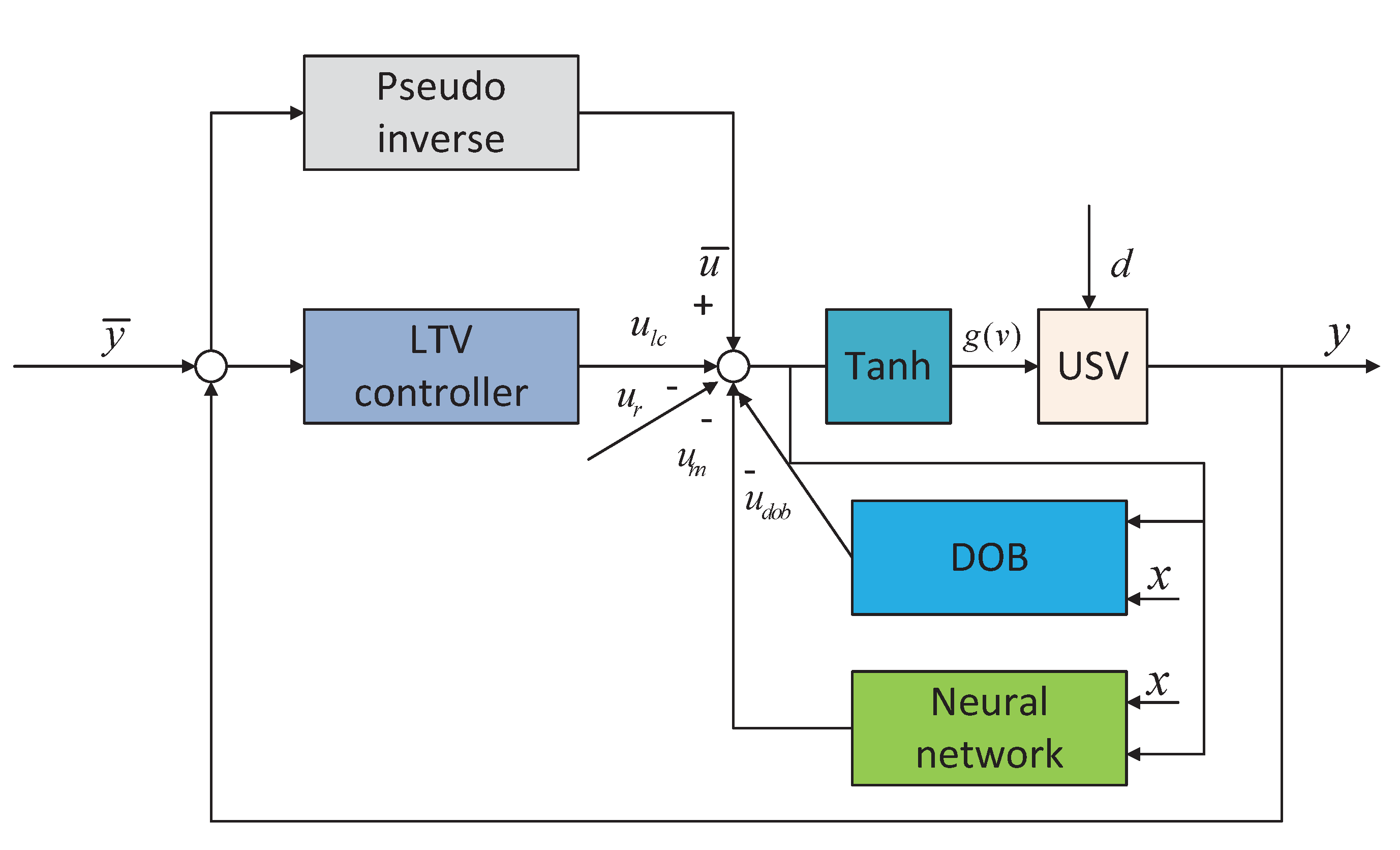
3. Design of Control Strategy

In this section, the main purpose is to design an adaptive course keeping control strategy with strong robustness based on TLC technology. Meanwhile, in order to improve the robustness of USV course control system, the disturbance observer is hired to compensate the external disturbance, and RBF neural network and an adaptive robust term are used to compensate the modeling error. Finally, the hyperbolic tangent function is introduced into the controlled system to solve the input saturation issue. The specific form and usage of RBF neural network can be referred to [36,37,38]. The framework of the course control strategy is described in Figure 3.

$u_r$ is a robust term employed to compensate for various errors, and $u_{nn}$ is the output of neural network to solve the modeling error issue. $u_{dob}$ is used to cope with environmental interference. $Tanh$ represents a hyperbolic tangent function to handle input saturation. $g(v)$ is the final control input.

Step 1: TLC strategy

Define the target course as ${\overline{x}}_1$, ${\dot{\overline{x}}}_1={\overline{x}}_2$, ${\overline{x}}_d={\left[\begin{array}{cc}{x}_{1d}& x_{2d}\end{array}\right]}^T$, $e_1=x-{\overline{x}}_d$. According to TLC theory, when $\Delta =0$ and $d=0$, $\overline{u}$ can be expressed as

$$\begin{array}{c}\hfill \overline{u}=\frac{1}{K}(T{\ddot{\overline{x}}}_1+{\dot{\overline{x}}}_1+\alpha {\dot{\overline{x}}}_1^3)\end{array}$$

(16)

The signal ${\overline{x}}_1$ is used to obtain ${\ddot{\overline{x}}}_1$ and ${\dot{\overline{x}}}_1$ through $G_1(s)=\frac{16s^2}{s^2+8s+16}$ and $G_2(s)=\frac{4s}{s+4}$ respectively to ensure the causality of the system. In addition, $A(t)=\left[\begin{array}{cc}0& 1\\ 0& -\frac{1}{T}-\frac{3\alpha }{T}{x}_2^2\end{array}\right]$ and $B(t)=\left[\begin{array}{c}0\\ \frac{K}{T}\end{array}\right]$ can be obtained from (5). On the basis of $PD$ spectrum theory, the desired closed-loop characteristics can be described as

$$\begin{array}{c}\hfill A_c=\left[\begin{array}{cc}0& 1\\ -{\omega }_n^2(t)& -2\zeta {\omega }_n(t)+\frac{{\dot{\omega }}_n(t)}{{\omega }_n(t)}\end{array}\right]\end{array}$$

(17)

where $\zeta$ is a constant damping, ${\omega }_n(t)$ is a time-varying bandwidth. The change rule of ${\omega }_n(t)$ is as follows: if $\left|x_1-{\overline{x}}_{1d}\right|\ge \frac{pi}{18}$, ${\omega }_n(t)=0.5$; if $0\le \left|x_1-{\overline{x}}_{1d}\right|<\frac{pi}{18}$, ${\omega }_n(t)=-\left|x_1-{\overline{x}}_{1d}\right|+0.5$.

Remark1. 

According to TLC theory, the bigger the ${\omega }_n(t)$ value, the bigger the bandwidth, the faster the error convergence. Therefore, the design principle of ${\omega }_n(t)$ is to use a larger bandwidth when the error is large, and when the error is gradually reduced, the bandwidth is also gradually reduced to avoid excessive overshoot, which is called variable bandwidth control.

After the above analysis and (7), $K(t)$ can be obtained.

$$\begin{array}{c}\hfill K(t)=\frac{T}{K}[-{\omega }_n^2(t),-2\zeta {\omega }_n(t)+{\dot{\omega }}_n(t)+\frac{1}{T}+\frac{3\alpha }{T}{x}_2^2]\end{array}$$

(18)

$u_{lc}$ can be obtained based on (6) and (18).

Step 2: Disturbance Observer

For (1), define $g_1(x)g_4(x)=g_2(x)$, $g_1(x)g_5(x)=g_3(x)$, $g_2(x)g_6(x)=g_3(x)$, and one can get that $g_4(x)=\frac{T}{K}$, $g_5(x)=\frac{\Delta T}{K}$ and $g_6(x)=\Delta$. In order to compensate external disturbance in real time, the disturbance observer is designed as (19).

$$\begin{array}{c}\hfill \left\{\begin{array}{c} {\dot{\widehat{x}}}_2=-\frac{1}{T}{x}_2-\frac{\alpha }{T}{x}_2^3+\widehat{d}+\frac{K}{T}u+k_1{\tilde{x}}_2\hfill \\ \dot{\widehat{d}}=k_2{\tilde{x}}_2\hfill \end{array}\right.\end{array}$$

(19)

where $k_1$ and $k_2$ are positive parameters to be designed, ${\tilde{x}}_2={\widehat{x}}_2-x_2$, $\tilde{d}=\widehat{d}-d$.

Based on the above analysis, the output of the disturbance observer can be described as

$$\begin{array}{c}\hfill u_{dob}=g_4(x)\widehat{d}\end{array}$$

(20)

Step 3: Adaptive Compensation

Define $e_1^{T}P(t)={\mathsf{\Theta }}_1$, $e_1^{T}P(t)g_2(x)={\mathsf{\Theta }}_2$ and $e_1^{T}P(t)g_3(x)={\mathsf{\Theta }}_3$, where $P(t)$ has the same meaning as (8). The output of neural network is selected as

$$\begin{array}{c}\hfill u_{nn}=g_5(x){\widehat{W}}^{T}h\end{array}$$

(21)

where $\widehat{W}$ is the estimated weight, h is a Gauss function. The estimation error can be defined as $\tilde{W}=W-\widehat{W}$. The adaptive law of neural network is

$$\begin{array}{c}\hfill \dot{\widehat{W}}=\mathsf{\Gamma }({\mathsf{\Theta }}_3+{\tilde{x}}_2)h+\kappa \mathsf{\Gamma }\widehat{W}\end{array}$$

(22)

where $\mathsf{\Gamma }$ and $\kappa$ are positive parameters to be designed. A robust term $u_r$ is employed to compensate for errors caused by neural network and disturbance observer to improve the robustness of the system, which can be defined as

$$\begin{array}{c}\hfill u_r=g_5(x)\widehat{\omega }\mathrm{sgn}({\mathsf{\Theta }}_2)\end{array}$$

(23)

The adaptive law of robust term is

$$\begin{array}{c}\hfill \dot{\widehat{\omega }}=\gamma {\mathsf{\Theta }}_2+\gamma \iota \widehat{\omega }\end{array}$$

(24)

where $\gamma$ and $\iota$ are the corresponding design parameters, and $\tilde{\omega }=\omega -\widehat{\omega }$.

Step 4: Input Saturation

Considering input saturation, the nonlinear model of USV can be rewritten as (25).

$$\begin{array}{c}\hfill \left\{\begin{array}{c} \dot{x}=f(x)+g_3(x)f(x)+g_1(x)g(v)+g_2(x)d+g_1(x)d_1(v)\hfill \\ y=x_1\hfill \end{array}\right.\end{array}$$

(25)

In order to facilitate the design of control law, auxiliary control signal w and the following auxiliary equation are introduced.

$$\begin{array}{c}\hfill \dot{v}=-cv+w\end{array}$$

(26)

where c is a positive parameter to be designed. Define ${\alpha }_u=\overline{u}+u_{lc}-u_{nn}-u_{dob}-u_r$, and enable ${\alpha }_u$ to obtain ${\dot{\beta }}_u$ through (10). Define error variable $e_2=g(v)-{\beta }_u$, and take the time derivative ${\dot{e}}_2$ along (12), we have

$$\begin{array}{c}\hfill {\dot{e}}_2=\dot{g}(v)-{\dot{\beta }}_u=\varsigma (-cv+w)-{\dot{\beta }}_u\end{array}$$

(27)

where $\varsigma =\frac{\partial g(v)}{\partial v}=\frac{4}{(e^{v/\phantom{v{u}_M}{u}_M}+e^{-v/\phantom{-\mathrm{v}{u}_M}{u}_M})}>0$. Since $\varsigma$ is variable, this increases the difficulty of design and analysis, so Nussbaum function $N(\epsilon )$ and auxiliary control law w are introduced into the design of the controller.

The control law w is selected as (28).

$$\begin{array}{c}\hfill w=N(\epsilon )\overline{w}\end{array}$$

(28)

where $\overline{w}=k_{eu}{e}_2-cv\varsigma -{\dot{e}}_2$, and $k_{eu}$ is a positive parameter. The Nussbaum function is defined as $N(\epsilon )={\epsilon }^{2}cos(\epsilon )$ and $\dot{\epsilon }={\lambda }_{\epsilon }\overline{w}{e}_2$. So far, the final control law has been designed.

4. Stability Analysis

Based on the course control law designed in Section 3, one can get (29).

$$\begin{array}{c}\hfill {\dot{e}}_1=A_C(t)e_1+R(·)+g_3(x)(\Delta f(x)-{\widehat{W}}^{T}h)+g_2(x)(d-\widehat{d}+\frac{K}{T}{d}_1-\widehat{\omega }\mathrm{sgn}({\mathsf{\Theta }}_2))\end{array}$$

(29)

where $R(·)$ expresses the high order term of the Tailorseries expansion [39], and satisfies

$$\begin{array}{c}\hfill ∥R(·)∥\le L{∥e_1∥}^2,\forall ∥e_1∥<\mu \end{array}$$

(30)

where L is a normal number. Define error variable $e_3$.

$$\begin{array}{c}\hfill e_3={\beta }_u-{\alpha }_u\end{array}$$

(31)

whose time derivative along (10) can be expressed by

$$\begin{array}{c}\hfill {\dot{e}}_3=-([A+f({\alpha }_u)+g({\alpha }_u)]{\beta }_u-[Bf({\alpha }_u)-Dg({\alpha }_u)])-{\dot{\alpha }}_u\end{array}$$

(32)

The meaning of all parameters in (32) is the same as that in (10). Define $B=D$, then (32) can be simplified as

$$\begin{array}{c}\hfill {\dot{e}}_3=-A_u{\beta }_u+B{\alpha }_u-{\dot{\alpha }}_u\end{array}$$

(33)

where $A_u=A+f({\alpha }_u)+g({\alpha }_u)$.

Remark2. 

${\dot{\alpha }}_u$ is bounded, and we assume that ${\dot{\alpha }}_u\le {\overline{\alpha }}_u$, where ${\overline{\alpha }}_u$ is normal number greater than zero.

Based on the design of control law and the above analysis, the main result of this paper is summarized as Theorem 1.

Theorem1. 

Consider the closed-loop system (25), the final control law $g(v)$, the adaptive laws (22) and (24), together with the disturbance compensation (20). If we choose ${\alpha }_2>1$ and ${\beta }_1>2L\mu {\alpha }_2$, all signals in the course control system are uniformly ultimately bounded (UUB).

ProofofTheorem1. 

Consider the following Lyapunov function candidate:

$$\begin{array}{c}\hfill V=\frac{1}{2}(e_1^{T}P(t)e_1+{\mathsf{\Gamma }}^{-1}{\tilde{W}}^T\tilde{W}+{\gamma }^{-1}{\tilde{\omega }}^2+\frac{1}{k_2}{\tilde{d}}^2+{\tilde{x}}_2^2+e_2^2+e_3^2)\end{array}$$

(34)

whose time derivative along (19), (28), (30) and (33) can be expressed by

$$\begin{array}{cc}\hfill \dot{V}& \le -\frac{1}{2}{e}_1^{T}Q(t)+{\tilde{W}}^T({\mathsf{\Theta }}_{3}h-{\mathsf{\Gamma }}^{-1}\dot{\widehat{W}})+{\mathsf{\Theta }}_{1}R(·)+{\mathsf{\Theta }}_2(g_6(x){\omega }_{nn}+\tilde{d}+\frac{K}{T}{d}_1-\widehat{\omega }\mathrm{sgn}({\mathsf{\Theta }}_2))\hfill \\ \hfill & -{\gamma }^{-1}\tilde{\omega }\dot{\widehat{\omega }}+\frac{1}{k_2}\tilde{d}\dot{\tilde{d}}+{\tilde{x}}_2{\dot{\tilde{x}}}_2+e_2{\dot{e}}_2-(A_u-\frac{\varpi }{2})e_3^2+\frac{{\overline{\alpha }}_u^2}{2\varpi }\hfill \end{array}$$

(35)

Define $B=A_u$, and we have $A_u{\beta }_u-A_u{\alpha }_u=A_u{e}_3$. $-e_3{\dot{\alpha }}_u\le \frac{\varpi e_3^2}{2}+\frac{{\overline{\alpha }}_u^2}{2\varpi }$ can be obtained from Young’s inequality, where $\varpi$ is a normal number.

$$\begin{array}{cc}\hfill \dot{V}& \le -\frac{1}{2}{e}_1^{T}Q(t)e_1+{\tilde{W}}^T({\mathsf{\Theta }}_{3}h-{\mathsf{\Gamma }}^{-1}\dot{\widehat{W}})+{\mathsf{\Theta }}_{1}R(·)+{\mathsf{\Theta }}_2(g_6(x)\epsilon +\tilde{d}+\frac{K}{T}{d}_1-\widehat{\omega }\mathrm{sgn}({\mathsf{\Theta }}_2))\hfill \\ \hfill & +{\gamma }^{-1}\tilde{\omega }\dot{\widehat{\omega }}+\frac{1}{k_2}\tilde{d}\dot{\tilde{d}}+{\tilde{x}}_2{\dot{\tilde{x}}}_2+e_2{\dot{e}}_2-(A_u-\frac{\varpi }{2})e_3^2+\frac{{\overline{\alpha }}_u^2}{2\varpi }\hfill \end{array}$$

(36)

With the disturbance observer (20), $\dot{V}$ yields

$$\begin{array}{cc}\hfill \dot{V}& \le -\frac{1}{2}{e}_1^{T}Q(t)e_1+{\tilde{W}}^T({\mathsf{\Theta }}_{3}h+{\tilde{x}}_{2}h-{\mathsf{\Gamma }}^{-1}\dot{\widehat{W}})+{\mathsf{\Theta }}_{1}R(·)+\tilde{\omega }(∥{\mathsf{\Theta }}_2∥-{\gamma }^{-1}\dot{\widehat{\omega }})-(k_1-\frac{1}{2}){\tilde{x}}_2^2\hfill \\ \hfill & +e_2{\dot{e}}_2-(A_u-\frac{\varpi }{2})e_3^2+\frac{{\overline{\alpha }}_u^2}{2\varpi }+\frac{1}{2}{\omega }_{nn}^2\hfill \end{array}$$

(37)

Submitting the adaptive laws (22), (24) yields

$$\begin{array}{cc}\hfill \dot{V}& \le -\frac{1}{2}{e}_1^{T}Q(t)e_1-\frac{\kappa }{2}{\tilde{W}}^2-\frac{\iota }{2}{\tilde{\omega }}^2-(k_1-\frac{1}{2}){\tilde{x}}_2^2-k_{eu}{e}_2^2+\frac{1}{{\lambda }_{\epsilon }}(\xi N(\epsilon )+1)\dot{\epsilon })+{\mathsf{\Theta }}_{1}R(·)\hfill \\ \hfill & +\frac{\kappa }{2}{W}^2+\frac{\iota }{2}{\omega }^2-(A_u-\frac{\varpi }{2})e_3^2+\frac{{\overline{\alpha }}_u^2}{2\varpi }+\frac{1}{2}{\omega }_{nn}^2\hfill \end{array}$$

(38)

Equation (39) can be obtained by further simplifying (38).

$$\begin{array}{cc}\hfill \dot{V}& \le -\frac{1}{2}({\beta }_1-2L\mu {\alpha }_2)e_1^2-\frac{\kappa }{2}{\tilde{W}}^2-\frac{\iota }{2}{\tilde{\omega }}^2-(k_1-\frac{1}{2}){\tilde{x}}_2^2-k_{eu}{e}_2^2-(A_u-\frac{\varpi }{2})e_3^2+\frac{1}{{\lambda }_{\epsilon }}(\xi N(\epsilon )+1)\dot{\epsilon })\hfill \\ \hfill & +\frac{\kappa }{2}{W}^2+\frac{\iota }{2}{\omega }^2+\frac{{\overline{\alpha }}_u^2}{2\varpi }+\frac{1}{2}{\omega }_{nn}^2\hfill \end{array}$$

(39)

Set $l_1=\frac{1}{2}({\beta }_1-2L\mu {\alpha }_2)>0$, $l_2=\frac{\kappa }{2}$, $l_3=\frac{\iota }{2}$, $l_4=k_1-\frac{1}{2}>0$, $l_5=-k_{eu}$, $l_6=A_u-\frac{\varpi }{2}>0$, $\mathsf{\Omega }=\frac{\kappa }{2}{W}^2+\frac{\iota }{2}{\omega }^2+\frac{{\overline{\alpha }}_u^2}{2\varpi }+\frac{1}{2}{\omega }_{nn}^2$, then (39) becomes

$$\begin{array}{c}\hfill \dot{V}\le -l_1{e}_1^2-l_2{\tilde{W}}^2-l_3{\tilde{\omega }}^2-l_4{\tilde{x}}_2^2-l_5{e}_2^2-l_6{e}_3^2+\mathsf{\Omega }+\frac{1}{{\lambda }_{\epsilon }}(\xi N(\epsilon )+1)\dot{\epsilon })\end{array}$$

(40)

Define $l=min\{l_1,l_2,l_3,l_4,l_5,l_6\}$, then it follows form (40) that

$$\begin{array}{c}\hfill \dot{V}\le -2lV+\mathsf{\Omega }+\frac{1}{{\lambda }_{\epsilon }}(\xi N(\epsilon )+1)\dot{\epsilon })\end{array}$$

(41)

Solving inequality (41) gives

$$\begin{array}{c}\hfill V\le V(0)e^{-2lt}+\frac{\mathsf{\Omega }}{2l}+\frac{{\int }_0^t(\xi N(\epsilon )+1)\dot{\epsilon }d\tau +C}{2l{\lambda }_{\epsilon }},\forall t>0\end{array}$$

(42)

Through the above proof, the following conclusion can be drawn: V is eventually bounded by $\frac{\mathsf{\Omega }}{2l}+\frac{{\int }_0^t(\xi N(\epsilon )+1)\dot{\epsilon }d\tau +C}{2l{\lambda }_{\epsilon }}$, thus all the error signals are UUB. □

5. Numerical Simulations

In this section, the proposed control scheme is compared with the classical PID control strategy by numerical simulation to verify its effectiveness and robustness. Meanwhile, the integrated time and absolute error (ITAE) index is used to describe course error to show the robustness of the proposed strategy, which is expressed as $ITAE={\int }_0^{t}t\left|x_1-{\overline{x}}_1\right|dt$ [40]. The research object of this paper is “Lanxin” USV of Dalian Maritime University, and its specific details and parameters can be referred to [41]. The control parameters are set to $u_M=35$ degrees, $\Delta =0.3$, $\zeta =0.707$, $k_1=1$, $k_2=30$, $\mathsf{\Gamma }=0.0001$, $\kappa =0.01$, $\gamma =0.2$, $\iota =0.001$, $c=100$, $k_{ue}=100$, ${\lambda }_{\epsilon }=0.4$, $A=1$, $B=D=1+f({\alpha }_u)+g({\alpha }_u)$.

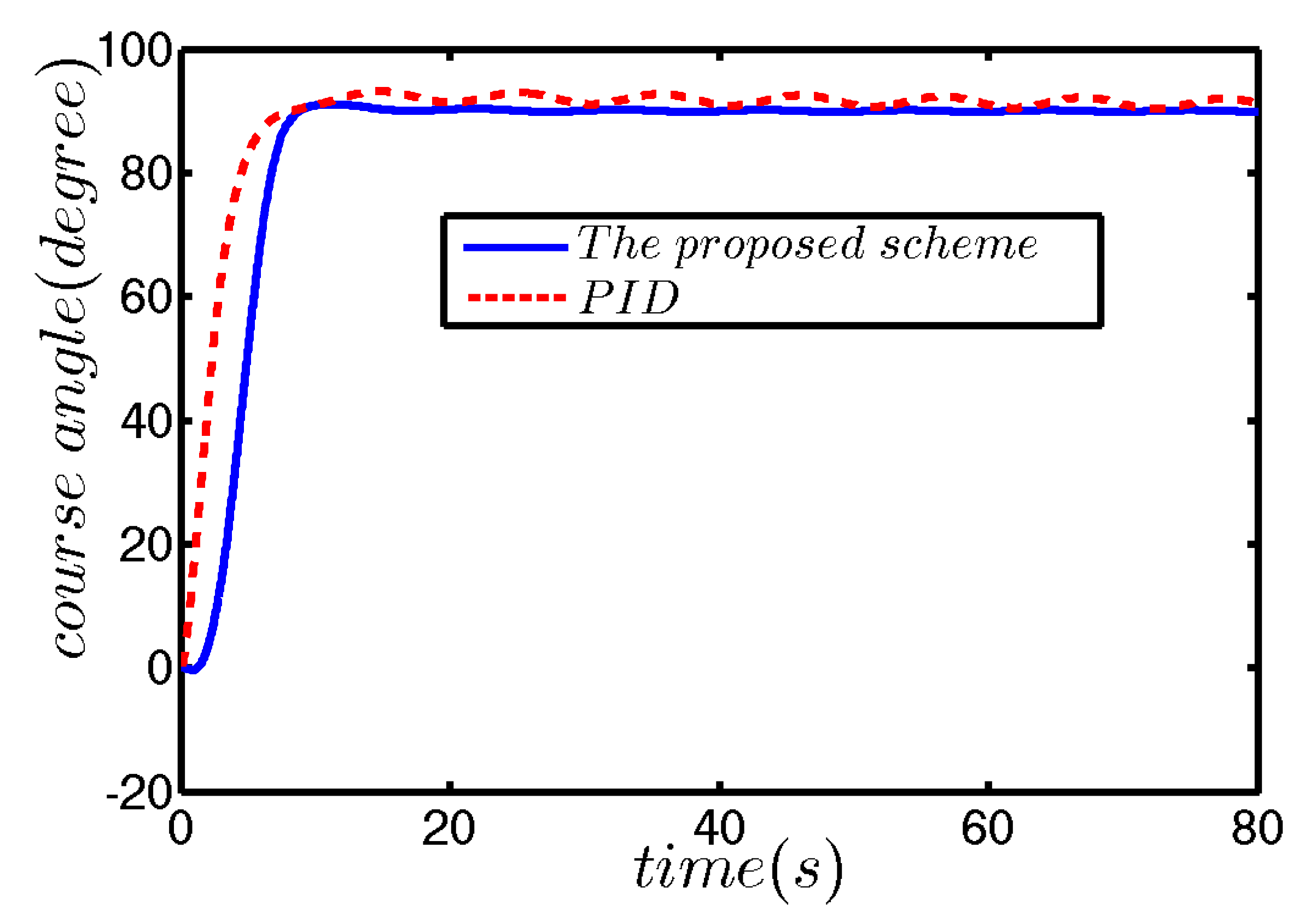
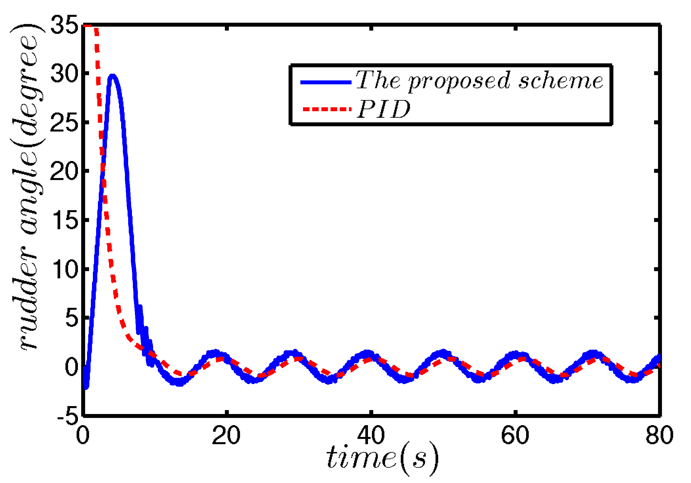
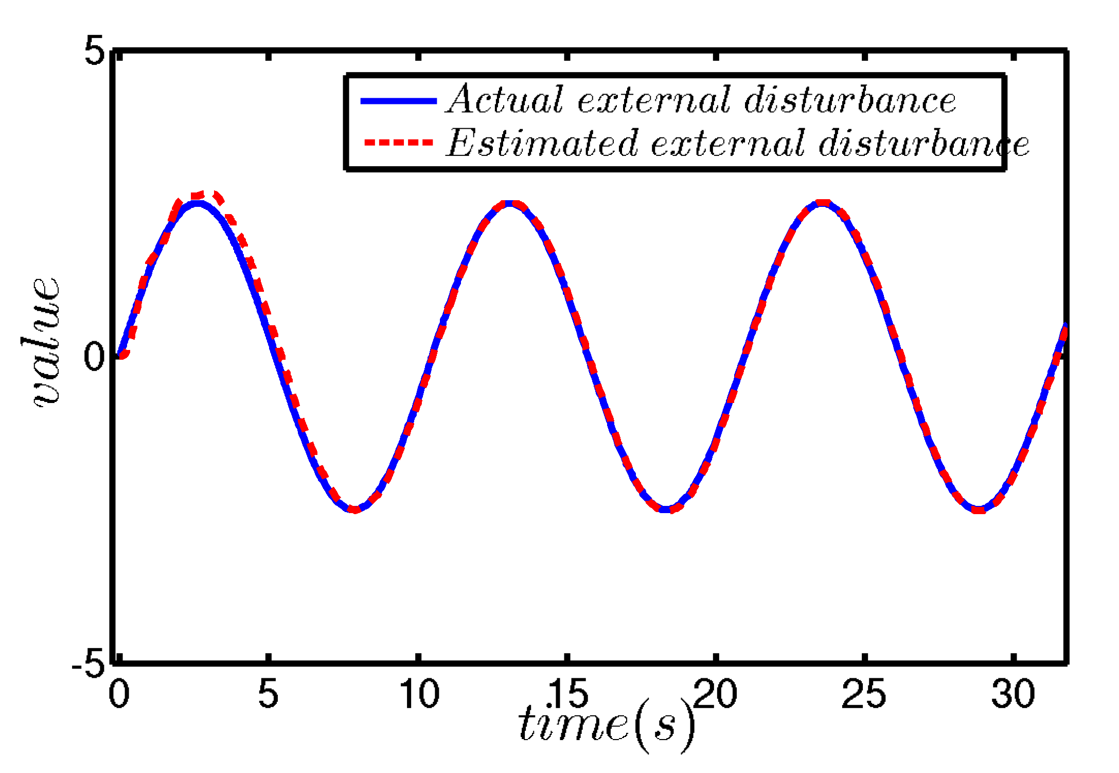
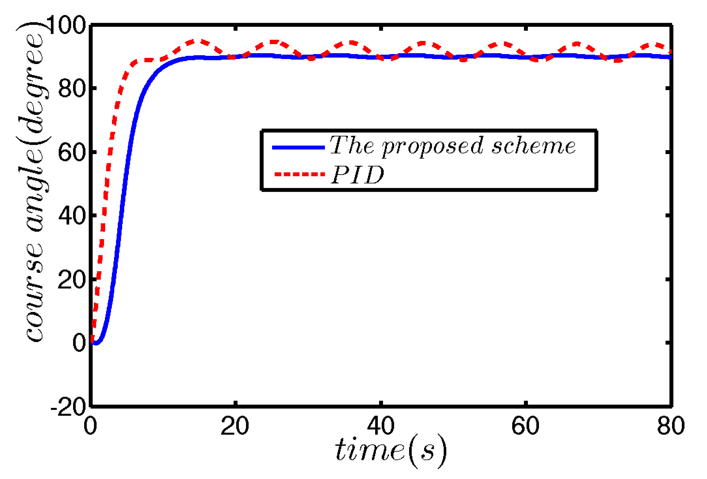
5.1. Weak External Disturbance

A weaker disturbance $d=2.5sin(0.6t)$ is introduced into the control system for simulation to verify the correctness of the control strategy proposed in this paper. Simulation results are provided in Figure 4, Figure 5 and Figure 6, and the ITAE index for course error is shown in

Table 1. Integrated time and absolute error (ITAE) index under weak disturbance.

ITAE	Value
The proposed scheme	1500
PID	5345

.

Figure 4 depicts the course keeping performance of the proposed scheme and PID strategy. The control strategy proposed in this paper can ensure that the course of USV is kept at the target value without obvious error, and it also maintains a faster convergence speed. However, the performance of the classic PID strategy is not ideal, and the USV’s course has been significantly fluctuating above and below the target value. It can be observed that the proposed scheme has better control performance than the PID strategy. Figure 5 shows the rudder angle curves of the proposed scheme and PID strategy. Obviously, in the early stage of control, the PID strategy has reached saturation (35 degrees), which means it needs more energy. Under the action of hyperbolic tangent function, the rudder angle curve of the proposed scheme does not reach 35 degrees and its change curve is relatively smooth. Compared with Figure 4, although the proposed scheme has a relatively gentle rudder angle curve, its convergence rate is not slower than that of PID strategy. Figure 6 plots actual and estimated external disturbances. The estimated curve can be well fitted with the actual curve, which shows the correctness of the proposed disturbance observer.

Furthermore, it can be seen from Table 1 that the ITAE index of the proposed strategy is 1500, which is only 28.1 percent of the PID strategy. These data further reflect the feasibility and superiority of the proposed scheme.

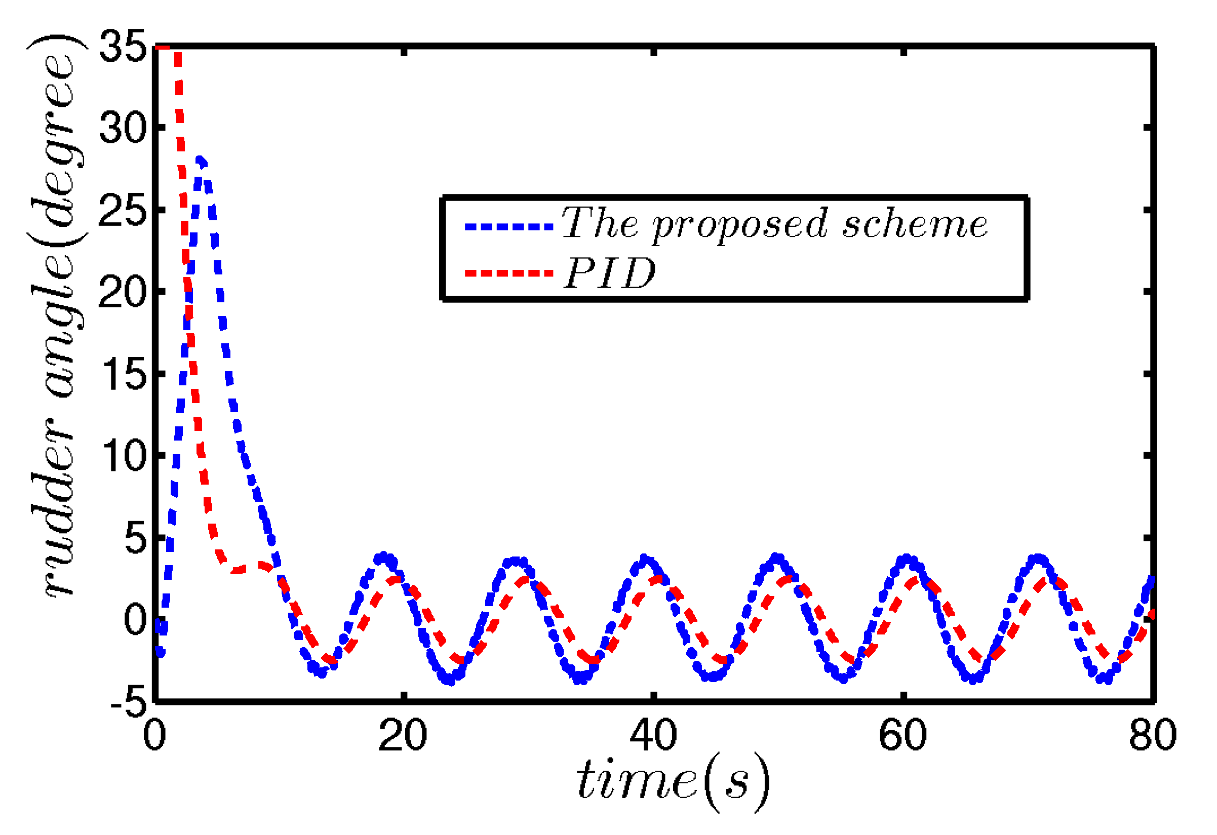
5.2. Strong External Disturbance

On the premise that any control parameters and initial conditions remain unchanged, the robustness of the proposed control strategy are verified by enhancing external disturbance. The enhanced external disturbance is $d=3\times 2.5sin(0.6t)$. The specific simulation results are shown in Figure 7, Figure 8 and Figure 9, and the ITAE index for course error is shown in

Table 2. ITAE index under strong disturbance.

ITAE	Value
The proposed scheme	1950
PID	6788

.

Figure 7 and Figure 8 depict the course control results and rudder angle curve of the proposed scheme and the PID strategy, respectively. It implies that compared with the PID strategy, the control strategy proposed in this paper still has better performance. It is worth noting that the course under the proposed strategy is still kept near the target value and there is no obvious fluctuation. Instead, the course error under PID control increases significantly compared to the result under weaker disturbance. The operation result of disturbance observer under strong disturbance is shown in Figure 9. Obviously, the disturbance observer presented in this paper has good performance in both strong and weak disturbances.

It can be seen from Table 2 that the ITAE index of the proposed strategy is 1950, which is only 28.7 percent of the PID strategy. Furthermore, the ITAE value of course error under strong external disturbance is only 450 higher than that under weak external disturbance, but the ITAE value of PID strategy increases by 1443. The robustness and effectiveness of the proposed control strategy are proved by simulation under weak and strong disturbances respectively.

6. Conclusions

This paper has presented a course keeping strategy with modeling error, external disturbance and input saturation. The scheme is proposed by combining the TLC strategy, RBF neural network, disturbance observer, hyperbolic tangent function and Nussbaum function, which is obviously different from traditional adaptive course control strategy. Based on the introduction of TLC technology into the control strategy, the neural network, the disturbance observer and the robust term improve the robustness of the system. Finally, the course keeping error is described by ITAE index: in the case of weak external disturbance, the ITAE index of the proposed scheme is only 28.1 percent of PID control; under strong external disturbance, the ITAE index of the proposed scheme is only PID control 28.7 percent, and only increased by 450. The feasibility and robustness of the proposed strategy are verified by numerical simulations.

Although this note has taken into account many practical situations, there are still many issues that need to be addressed. For example, the disturbance observer designed in this paper can only estimate the slow time-varying disturbance, but the estimation effect of the non-slow time-varying disturbance is not satisfactory. Or, the dynamic characteristics of the actuator are not taken into account, which is one of the future research directions of the author.

References

1. Zaghi, S.; Dubbioso, G.; Broglia, R.; Muscari, R. Hydrodynamic characterization of USV vessels with innovative SWATH configuration for coastal monitoring and low environmental impact. Transp. Res. Procedia 2016, 14, 1562–1570. [Google Scholar] [CrossRef] [Green Version]
2. Sun, X.; Wang, G.; Fan, Y.; Mu, D.; Qiu, B. Collision Avoidance Using Finite Control Set Model Predictive Control for Unmanned Surface Vehicle. Appl. Sci. 2018, 926. [Google Scholar] [CrossRef] [Green Version]
3. Han, J.; Xiong, J.; He, Y.; Gu, F.; Li, D. Nonlinear Modeling for a Water-Jet Propulsion USV: An Experimental Study. IEEE Trans. Ind. Electron. 2017, 64, 3348–3358. [Google Scholar] [CrossRef]
4. Brossard, J.; Bensoussan, D.; Landry, R.; Hammami, M. Robustness studies on quadrotor control. In Proceedings of the IEEE International Conference on Unmanned Aircraft Systems (ICUAS 2019), Atlanta, GA, USA, 11–14 June 2019; pp. 344–352. [Google Scholar]
5. Mystkowski, A. An application of mu-synthesis for control of a small air vehicle and simulation results. J. Vibroeng. 2012, 14, 79–86. [Google Scholar]
6. Tunik, A.A.; Nadsadnaya, O.I. A Flight Control System for Small Unmanned Aerial Vehicle. Int. Appl. Mech. 2018, 54, 239–247. [Google Scholar] [CrossRef]
7. Wang, Y.L.; Han, Q.L. Network-based heading control and rudder oscillation reduction for unmanned surface vehicles. IEEE Trans. Control Syst. Technol. 2017, 25, 1609–1620. [Google Scholar] [CrossRef]
8. Miao, R.; Dong, Z.; Wan, L.; Zeng, J. Heading Control System Design for a Micro-USV Based on an Adaptive Expert S-PID Algorithm. Pol. Marit. Res. 2018, 25, 6–13. [Google Scholar] [CrossRef] [Green Version]
9. Fossen, T.I. Handbook of Marine Craft Hydrodynamics and Motion Control; Wiley: New York, NY, USA, 2011; ISBN 978-1119991496. [Google Scholar]
10. Zhang, X.K.; Zhang, Q.; Ren, H.X.; Yang, G.P. RLinear reduction of backstepping algorithm based on nonlinear decoration for ship course-keeping control system. Ocean Eng. 2018, 147, 1–8. [Google Scholar] [CrossRef]
11. Witkowska, A.; Śmierzchalski, R. Adaptive dynamic control allocation for dynamic positioning of marine vessel based on backstepping method and sequential quadratic programming. Ocean Eng. 2018, 163, 570–582. [Google Scholar] [CrossRef]
12. Mu, D.; Wang, G.; Fan, Y.; Qiu, B.; Sun, X. Stereovision-based target tracking system for USV operations. Appl. Sci. 2018, 8, 547. [Google Scholar] [CrossRef] [Green Version]
13. Mizuno, N.; Saka, N.; Katayama, T. A ship’s automatic maneuvering system using optimal preview sliding mode controller with adaptation mechanism. IFAC-PapersOnLine 2016, 49, 576–581. [Google Scholar] [CrossRef]
14. Liu, Z. Ship adaptive course keeping control with nonlinear disturbance observer. IEEE Access 2017, 5, 17567–17575. [Google Scholar] [CrossRef]
15. Videcoq, E.; Girault, M.; Bouderbala, K.; Nouira, H.; Salgado, J.; Petit, D. Parametric investigation of Linear Quadratic Gaussian and Model Predictive Control approaches for thermal regulation of a high precision geometric measurement machine. Appl. Therm. Eng. 2015, 78, 720–730. [Google Scholar] [CrossRef]
16. Mu, D.; Zhao, Y.; Wang, G.; Fan, Y. USV model identification and course control. In Proceedings of the 2016 IEEE Sixth International Conference on Information Science and Technology (ICIST), Dalian, China, 6–8 May 2016; pp. 263–267. [Google Scholar]
17. Lei, Z.; Guo, C. Disturbance rejection control solution for ship steering system with uncertain time delay. Ocean Eng. 2015, 95, 78–83. [Google Scholar] [CrossRef]
18. Kahveci, N.E.; Ioannou, P.A. Adaptive steering control for uncertain ship dynamics and stability analysis. Automatica 2013, 49, 685–697. [Google Scholar] [CrossRef]
19. Peng, Z.; Wang, D.; Wang, W.; Liu, L. Neural adaptive steering of an unmanned surface vehicle with measurement noises. Neurocomputing 2016, 186, 228–234. [Google Scholar] [CrossRef]
20. Zhang, X.K.; Zhang, G.Q. Design of Ship Course-Keeping Autopilot using a Sine Function-Based Nonlinear Feedback Technique. J. Navig. 2016, 69, 246–256. [Google Scholar] [CrossRef] [Green Version]
21. Fan, Y.; Mu, D.; Zhang, X.; Guo, C.; Wang, G. Course keeping Control Based on Integrated Nonlinear Feedback for a USV with Pod-like Propulsion. J. Navig. 2018, 71, 878–898. [Google Scholar] [CrossRef]
22. Mu, D.; Wang, G.; Fan, Y.; Zhao, Y. Modeling and identification of podded propulsion unmanned surface vehicle and its course control research. Math. Probl. Eng. 2017, 2017, 3209451. [Google Scholar] [CrossRef]
23. Chen, M.; Ge, S.S.; Ren, B. Adaptive tracking control of uncertain MIMO nonlinear systems with input constraints. Automatica 2011, 47, 452–465. [Google Scholar] [CrossRef]
24. Norrbin, N.H. Ship manoeuvring with application to shipborne predictors and real-time simulators. Arch. J. Mech. Eng. Sci. 1972, 14, 1959–1982. [Google Scholar] [CrossRef]
25. Chen, Y.; Zhu, J.J. Car-Like Ground Vehicle Trajectory Tracking by Using Trajectory Linearization Control. In Proceedings of the ASME 2017 Dynamic Systems and Control Conference. American Society of Mechanical Engineers, Tysons, VA, USA, 11–13 October 2017; p. V002T21A014. [Google Scholar]
26. Liu, Y.; Wu, X.; Zhu, J.J.; Lwe, J. Omni-directional mobile robot controller design by trajectory linearization. In Proceedings of the IEEE American Control Conference, Denver, CO, USA, 4–6 June 2003; Volume 4, pp. 3423–3428. [Google Scholar]
27. Zhao, Y.; Zhu, J.J. Automatic Aircraft Loss-of-Control Prevention by Bandwidth Adaptation. J. Guid. Control Dyn. 2016, 40, 878–889. [Google Scholar] [CrossRef]
28. Zhao, Y.; Zhu, J.J. Aircraft loss-of-control autonomous recovery: Mission trajectory tracking restoration. In Proceedings of the 2016 International Conference on Unmanned Aircraft Systems (ICUAS), Arlington, VA, USA, 7–10 June 2016; pp. 801–810. [Google Scholar]
29. Liu, Y.; Zhu, J.J.; Williams, R.L., II; Wu, J. Omni-directional mobile robot controller based on trajectory linearization. Robot. Auton. Syst. 2008, 56, 461–479. [Google Scholar] [CrossRef]
30. Yali, X.; Changsheng, J. Trajectory linearization control of an aerospace vehicle based on RBF neural network. J. Syst. Eng. Electron. 2008, 19, 799–805. [Google Scholar] [CrossRef]
31. Grossberg, S. Nonlinear neural networks: Principles, mechanisms, and architectures. Neural Netw. 1988, 1, 17–61. [Google Scholar] [CrossRef] [Green Version]
32. Pan, C.Z.; Lai, X.Z.; Yang, S.X.; Wu, M. A biologically inspired approach to tracking control of underactuated surface vessels subject to unknown dynamics. Expert Syst. Appl. 2015, 42, 2153–2161. [Google Scholar] [CrossRef]
33. Wen, C.; Zhou, J.; Liu, Z.; Su, H. Robust adaptive control of uncertain nonlinear systems in the presence of input saturation and external disturbance. IEEE Trans. Autom. Control 2011, 56, 1672–1678. [Google Scholar] [CrossRef]
34. Chen, C.; Liu, Z.; Zhang, Y.; Chen, C.L.P.; Xie, S. Saturated Nussbaum Function Based Approach for Robotic Systems with Unknown Actuator Dynamics. IEEE Trans. Cybern. 2016, 46, 2311–2322. [Google Scholar] [CrossRef]
35. Xudong, Y.; Jingping, J. Adaptive nonlinear design without a priori knowledge of control directions. IEEE Trans. Autom. Control 1998, 43, 1617–1621. [Google Scholar] [CrossRef]
36. Han, S.S.; Wang, H.P.; Tian, Y.; Christov, N. Time-delay estimation based computed torque control with robust adaptive RBF neural network compensator for a rehabilitation exoskeleton. ISA Trans. 2020, 97, 171–181. [Google Scholar] [CrossRef]
37. Shi, X.Y.; Cheng, Y.H.; Yin, C.; Huang, X.G. Design of adaptive backstepping dynamic surface control method with RBF neural network for uncertain nonlinear system. Neurocomputing 2019, 30, 490–503. [Google Scholar] [CrossRef]
38. Heshmati-Alamdari, S.; Nikou, A.; Dimarogonas, D.V. Robust Trajectory Tracking Control for Underactuated Autonomous Underwater Vehicles in Uncertain Environments. IEEE Trans. Autom. Sci. Eng. 2020. [Google Scholar] [CrossRef]
39. Khalil, H.K.; Grizzle, J.W. Noninear Systems; Prentice-Hall: Upper Saddle River, NJ, USA, 1996. [Google Scholar]
40. Xu, J.X.; Li, C.; Hang, C.C. Tuning of fuzzy PI controllers based on gain/phase margin specifications and ITAE index. ISA Trans. 1996, 35, 79–91. [Google Scholar]
41. Mu, D.; Wang, G.; Fan, Y.; Sun, X.; Qiu, B. Modeling and Identification for Vector Propulsion of an Unmanned Surface Vehicle: Three Degrees of Freedom Model and Response Model. Sensors 2018, 18, 1889. [Google Scholar] [CrossRef] [Green Version]
Figure 1. Block diagram of trajectory linearization control (TLC) technology.
Energies 13 05091 g001
Figure 2. The principle of input saturation.
Energies 13 05091 g002
Figure 3. Logic Diagram of course control strategy.
Energies 13 05091 g003
Figure 4. The curves of course angle under weak disturbance.
Energies 13 05091 g004
Figure 5. The curves of rudder angle under weak disturbance.
Energies 13 05091 g005
Figure 6. The curves of disturbance estimation under weak disturbance.
Energies 13 05091 g006
Figure 7. The curves of course angle under strong disturbance.
Energies 13 05091 g007
Figure 8. The curves of rudder angle under strong disturbance.
Energies 13 05091 g008
Figure 9. The curves of disturbance estimation under strong disturbance.
Energies 13 05091 g009