Thermal Analysis Strategy for Axial Permanent Magnet Coupling Combining FEM with Lumped-Parameter Thermal Network

Abstract

Thermal analysis is exceptionally important for operation safety of axial permanent magnet couplings (APMCs). Combining a finite element method (FEM) with a lumped-parameter thermal network (LPTN) is an effective yet simple thermal analysis strategy for an APMC that is developed in this paper. Also, some assumptions and key considerations are firstly given before analysis. The loss, as well as the magnetic field distribution of the conductor sheet (CS) can be accurately calculated through FEM. Then, the loss treated as source node loss is introduced into the LPTN model to obtain the temperature results of APMCs, where adjusting conductivity of the CS is a necessary and significant link to complete an iterative calculation process. Compared with experiment results, this thermal analysis strategy has good consistency. In addition, a limiting and safe slip speed can be determined based on the demagnetization temperature permanent magnet (PM).

1. Introduction

Permanent magnet couplings (PMCs) as a new transmission topology can be employed in several industrial applications, such as conveyors, fans, pumps and braking devices [1,2,3]. Also, PMCs offer many advantages, such as no physical contact, soft starting, shock isolation, and misalignment tolerance, which all taken together provide better protection for mechanical systems [4,5]. Typically, there are two configurations of PMCs: axial [6,7,8] and radial [9,10,11] type, both with the above-mentioned advantages. In this work, we pay attention to axial permanent magnet coupling (APMC) as depicted in Figure 1. It is divided into two parts: one is the permanent magnet (PM) module including a PM holder and several PMs (generally Nd-Fe-B type), and the other is the conductor sheet (CS) module, generally manufactured with copper. Additionally, there are two other iron yokes to make the magnetic fluxes close corresponding the PM holder and the CS, respectively.

In [3,6,12,13], the operating principle of APMCs was introduced in detail. On account of having the slip (s = n_in − n_out) between the CS module and the PM module, the eddy currents, which are generated on the CS, interact with the original magnetic field of PMs and induce an effective torque. Meanwhile, the temperature rise, especially at the low-slip condition, is inevitable due to the generated-currents. Surpassing the thermal limit of PMs involves the risk of irreversible demagnetization, while the excessive temperature can also damage other components. Beside the precaution of each component destruction, intensive thermal stress can shorten equipment lifetime. Therefore, thermal analysis is absolutely necessary both for the design stage and the monitoring stage of APMCs. Given the high-speed rotation characteristics of APMCs, analyzing the components’ temperature imposes a greater challenge.

Today, APMCs have been investigated for a long time, and a number of papers can be discovered in [14,15,16,17,18,19,20,21,22]. Research in [16] and [17], based on a two-dimensional (2-D) approximation of the magnetic field distribution, a practical and effective analytical calculation approach for the torque performance of APMCs, was proposed. Given the three-dimensional (3-D) edge effects and curvature effects, a 3-D analytical model was developed in [19] and [22] to compute the torque and the axial force. Obviously, all of studies mentioned above are focused on the torque analysis ignoring the thermal influence since APMCs belong to a kind of transmission device ultimately.

Unfortunately, thermal analysis to APMCs is not easy work due to the property variation of each component with temperature that result in mathematical difficulties. Hence, it is then acceptable to find very little literature about this. Here, good news is that there are some methods from PM motors to be borrowed [23,24,25,26]. In general, thermal analysis can be segmented into two primary means: numerical methods and thermal network. The former, such as finite-element method (FEM), not only can obtain the temperature distribution accurately, but also can take the actual 3D geometry and material properties into account. However, for the analysis objects, which have complex topologies or contain components equipped with highly diverse thermal characteristics, FEM is difficult to simplify [27]. Consequently, the mesh is refined and enormous, resulting in having a heavy expense in computer resources and being time-consuming, which then hampers the application of FEM in rapid optimization [28]. The latter is a lumped–parameter approach offering the advantages of economy, flexibility and simplicity. Nevertheless, it cannot acquire the temperature distribution in detail and heavily depends on the precise thermal parameters of the loss and heat coefficient (conduction, radiation and convection) [29,30]. For the aforementioned studies, however, the study methods are not fully applicable to the thermal analysis of APMCs.

From the perspective of engineering application and operation safety for APMCs, it is important to have a simplified and accurate thermal analysis strategy in order to quickly obtain the temperature distribution of APMCs. In this paper, FEM and lumped-parameter thermal network (LPTN) are combined to effectively calculate the temperature results of APMCs. The remainder of the paper is organized as follows: Section 2 presents the geometry of the studied APMC. In Section 3, the proposed strategy and assumptions are offered. The magnetic field model, including the loss results is established in Section 4. Then, Section 5 gives the LPTN model to obtain the temperature results. Finally, Section 6 concludes the work of this paper.

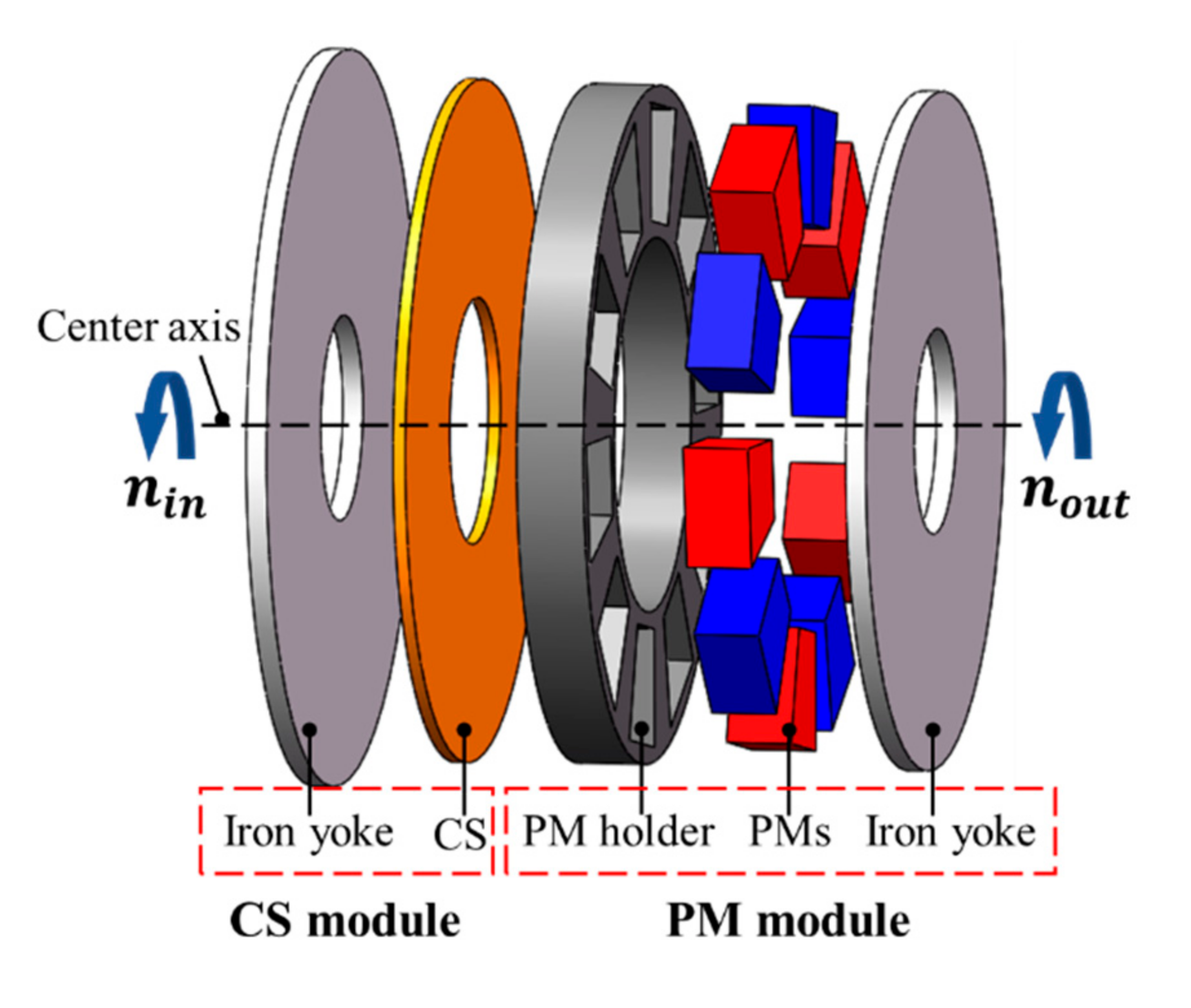
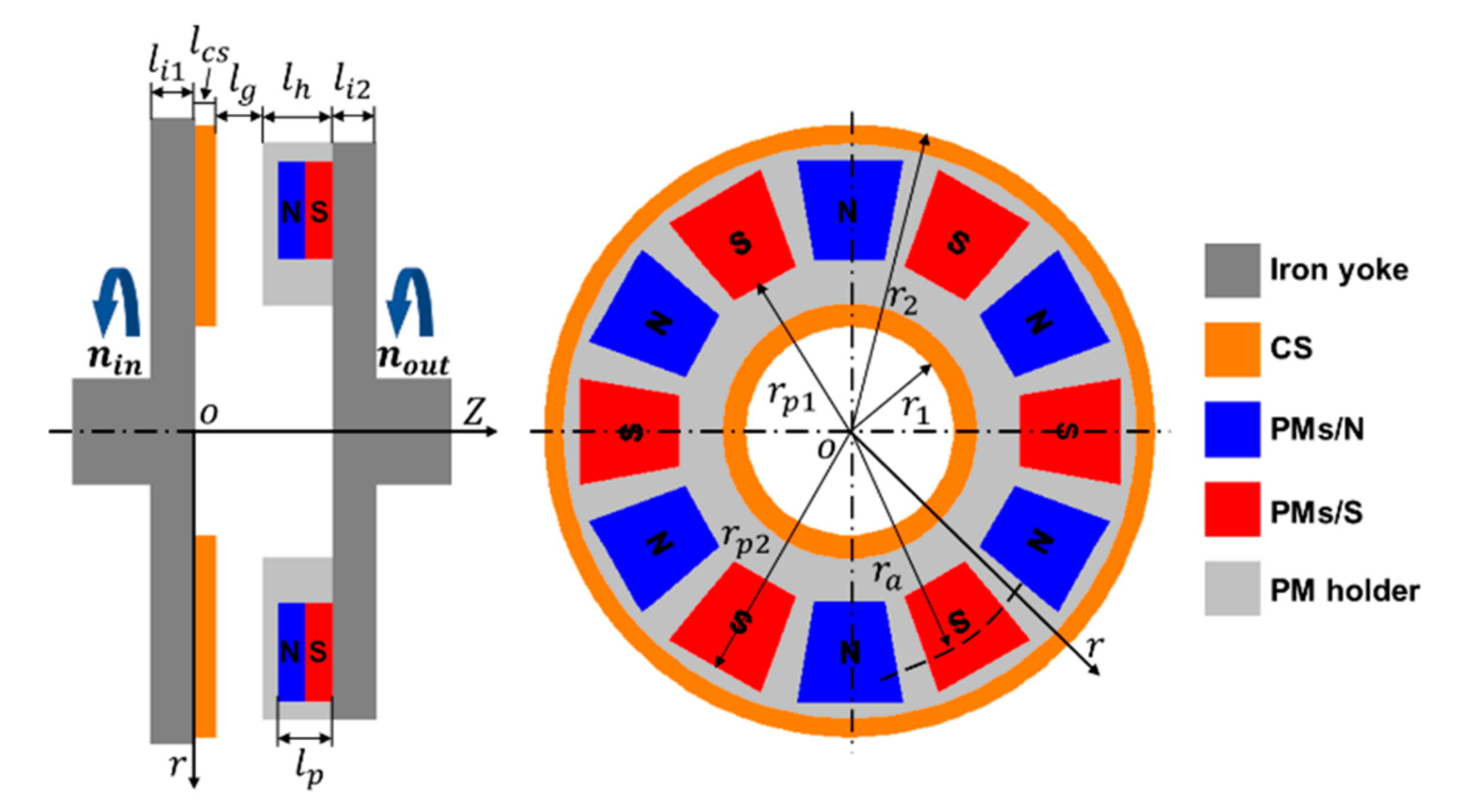
2. Geometry of the Studied APMC

Figure 2 provides the geometry of the studied APMC as well as its exploded view and geometrical parameters, where the pole-pairs number of the PMs is supposed to be 6. Here, l_g is adjustable and generally ranges from 3 mm to 8 mm. In the PM holder, the fan-shaped PMs are arranged in accordance with a N/S alternating sequence. The major parameters of the studied APMC are given in

Table 1. Parameters of the studied APMC.

Symbol	Meaning	Value
li1	Thickness of the iron yoke (CS side)	10 mm
li2	Thickness of the iron yoke (PM side)	10 mm
lcs	Thickness of the CS	6 mm
lg	Thickness of the air-gap	3–8 mm
lh	Thickness of the PM holder	26 mm
lp	Thickness of the PM	25 mm
r1	Inside radius of the CS	87.5 mm
r2	Outside radius of the CS	187.5 mm
rp1	Inside radius of the PM	115 mm
rp2	Outside radius of the PM	165 mm
ra	Average radius of the PM	140 mm
Hp	Coercive force of the PM	−900 KA/m
σcs	Conductivity of the CS	5.8 × 107 S/m (20 °C)

. These parameters are derived from some reliable engineering design experience and its detailed design thought can be referred to [3,4,6]. Given the adjustable air-gap and these parameters, the manufactured prototype of the studied APMC was built and put on the cast-iron platform, as shown in Figure 3.

3. Proposed Strategy and Assumptions

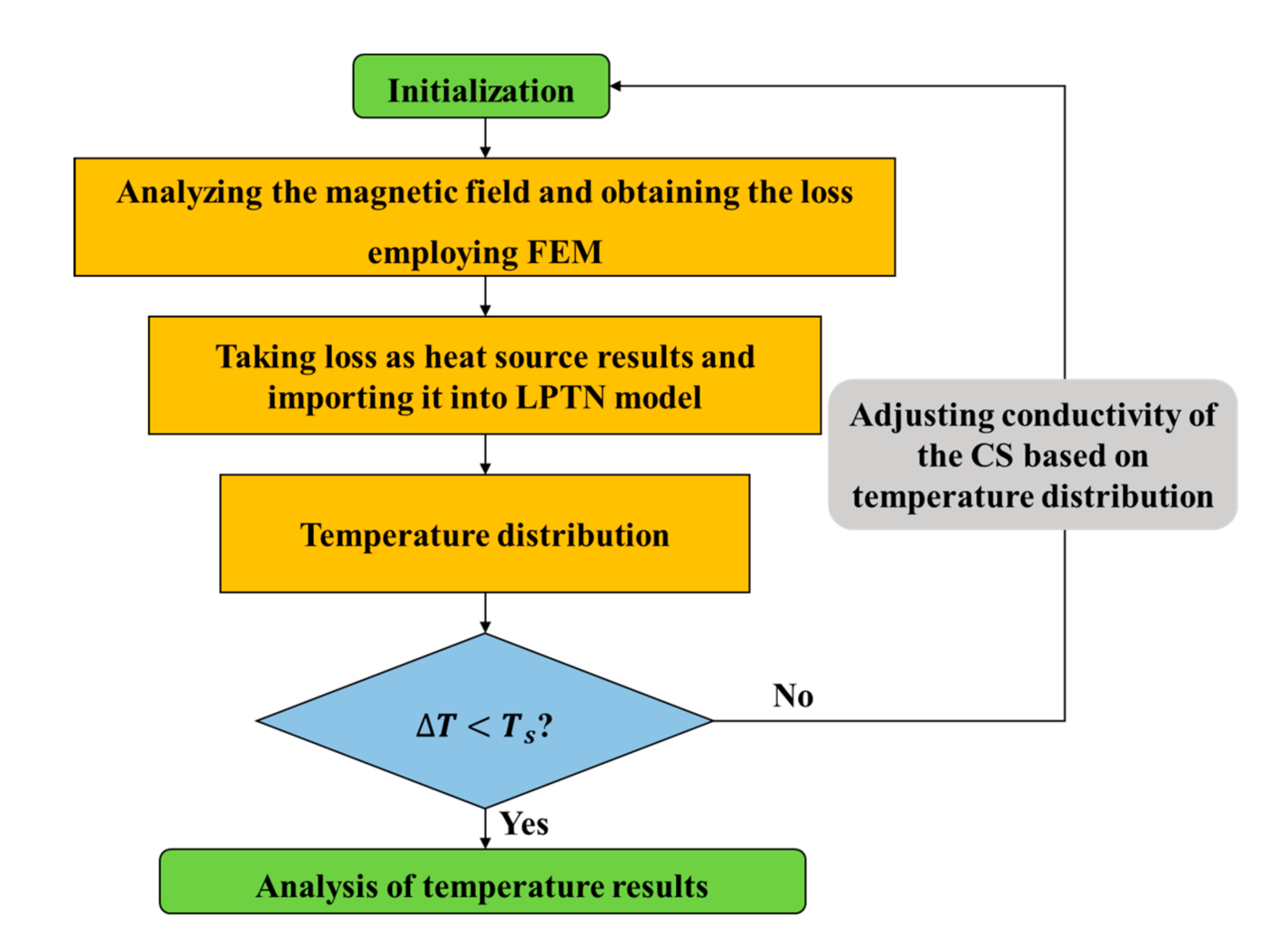
3.1. Proposed Strategy

Figure 4 describes the procedure of the proposed thermal analysis strategy. Since the conductivity of the CS is closely related to temperature, this procedure is an iterative updating calculation. After initialization and referring to the parameters in Table 1, the magnetic field result is obtained as well as the loss employing FEM. Then, regarding the loss as the heat source, the LPTN model is employed to calculate the temperature distribution. Thanks to the temperature obtained each time being different, so in each iteration, the conductivity of the CS was updated according to its temperature characteristic. Based on the updated conductivity, the thermal analysis re-executed until the temperature convergence threshold is satisfied. Herein, ΔT is the percentage error of each component temperature relative to the previous calculation, and T_s is the set convergence threshold, such as 1%.

3.2. Assumptions

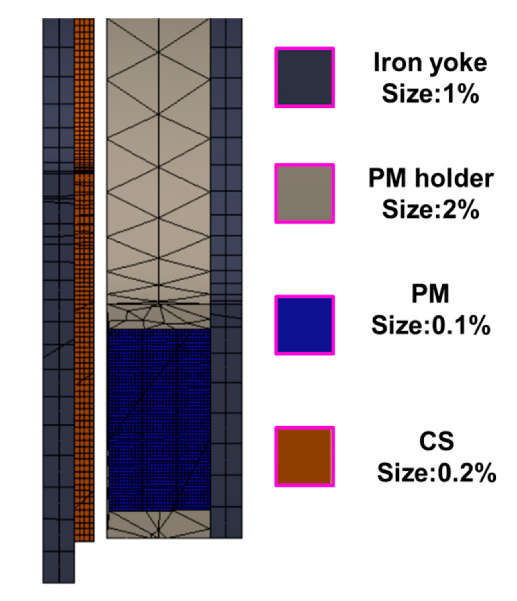
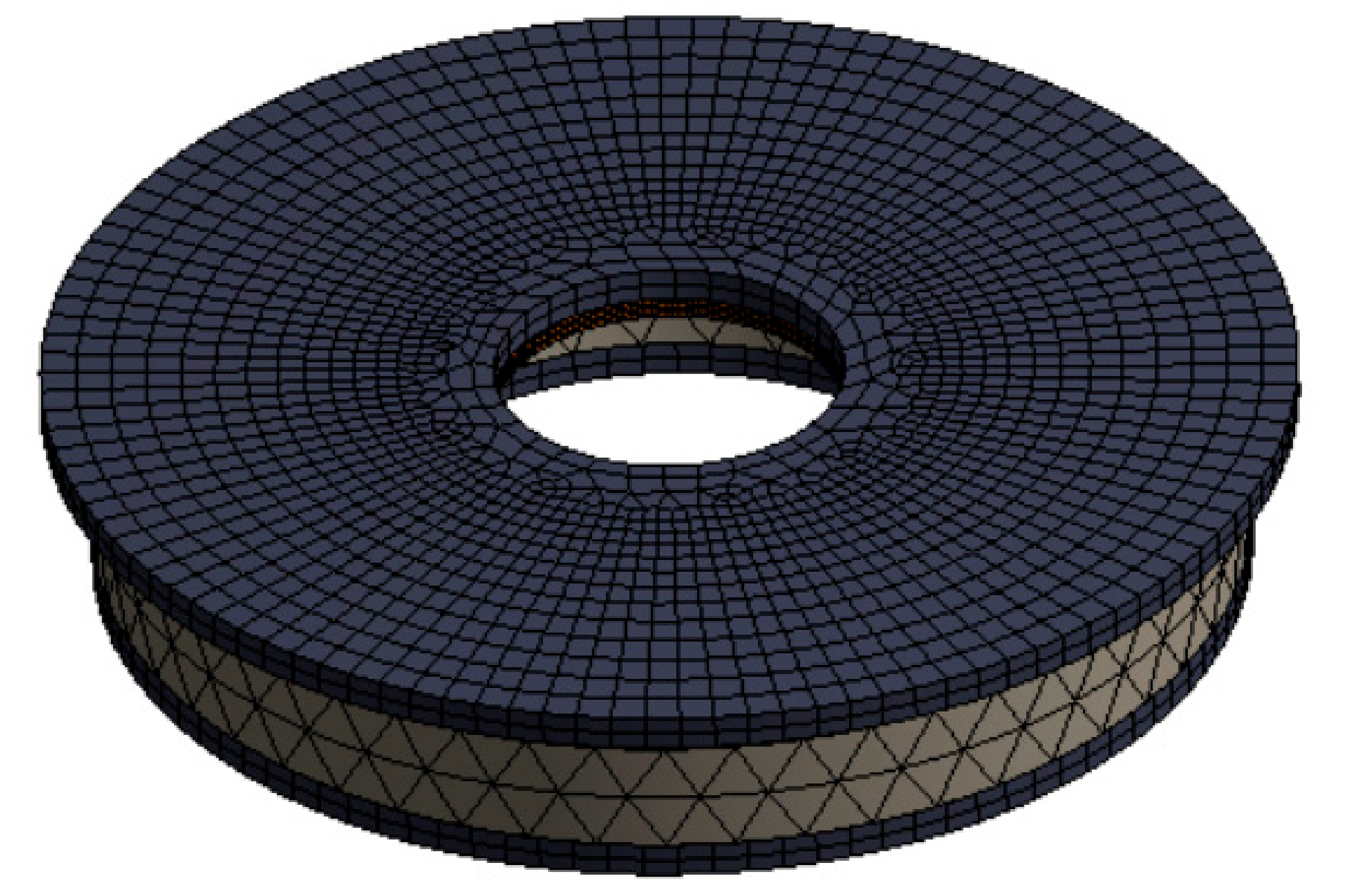
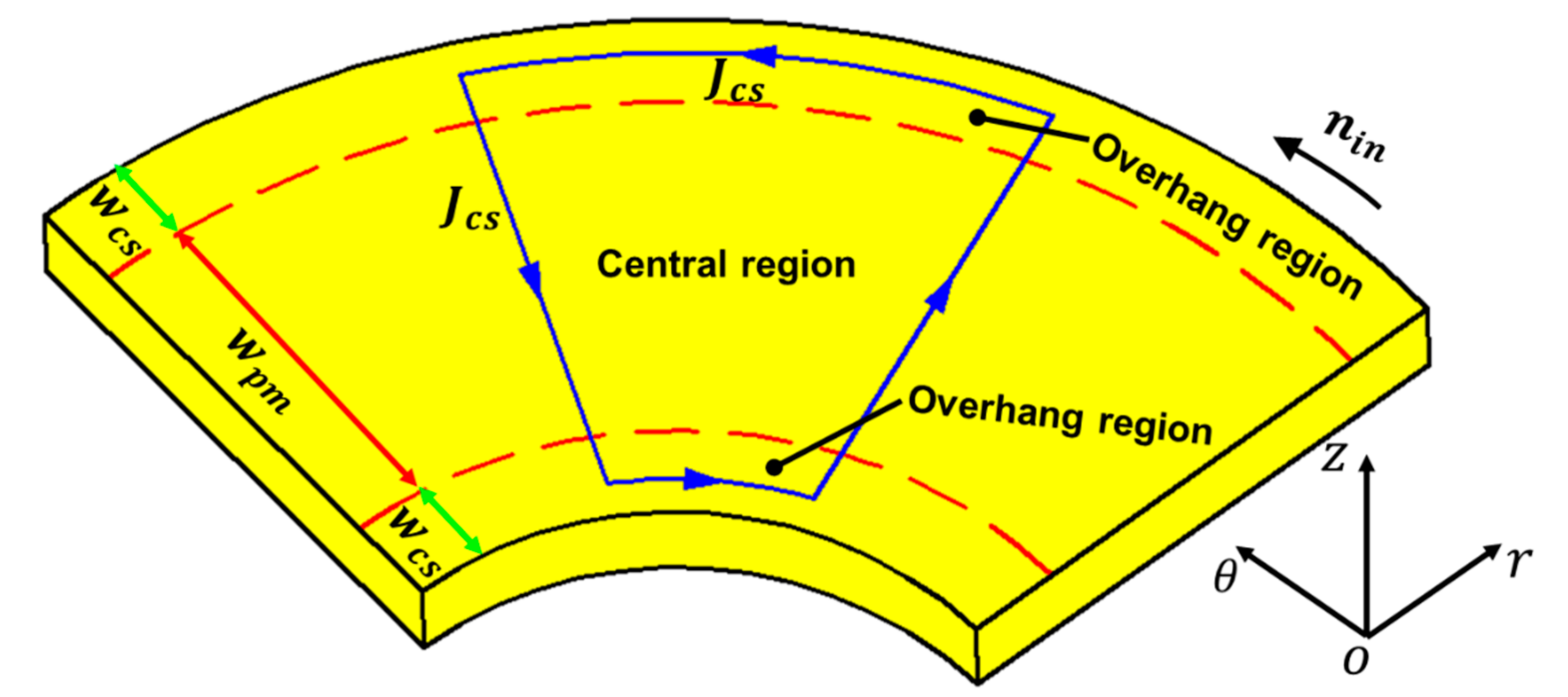
• From Figure 2, the geometry of the APMC is approximatively centrosymmetric. Also, the parameters of every component along the circumferential direction (r) were uniform. Therefore, the loss and temperature distributions were centrosymmetric as well.
• The APMC operated in the steady-state with a certain slip speed (s), so it is reasonable to think the air in the air-gap as stable, whereby the temperature distribution in the air-gap was also the same.
• Considering the skin effect, the loss is mainly concentrated upon the CS, and other losses, were ignored.

4. Magnetic Field Model

4.1. Key Considerations

In this section, we employ the FEM software Ansoft Maxwell 3D (v16, ANSYS Inc, Canonsburg, Pennsylvania, USA.) to model the magnetic field of the APMC. Assigning H_p and σ_cs in Table 1 to the PMs and the CS respectively is the first important consideration, where σ_cs is a parameter to be adjusted from Figure 4 and valued at room temperature (20 ℃) initially. As important as the PM and the CS, the magnetic characteristic of the iron yokes (B-H curve) should also be considered in the FEM, as exposed in Figure 5. Additionally, Figure 6 shows the mesh size for all the components, following a certain proportion. Here, from the perspective of simulation precision, the CS and the PMs are meshed detailedly. Figure 7 shows the mesh in 3D of the FEM model, where this model includes 570,979 nodes and 119,316 elements.

Besides, considering the convergence of this FEM results, the simulation step can be given by

$$t_{step}=(1.2~1.5)\frac{60}{1000s}$$

(1)

wherein, the coefficient (1.2~1.5) indicates that the CS module has rotated 1.2 to 1.5 turns relative to the PM module.

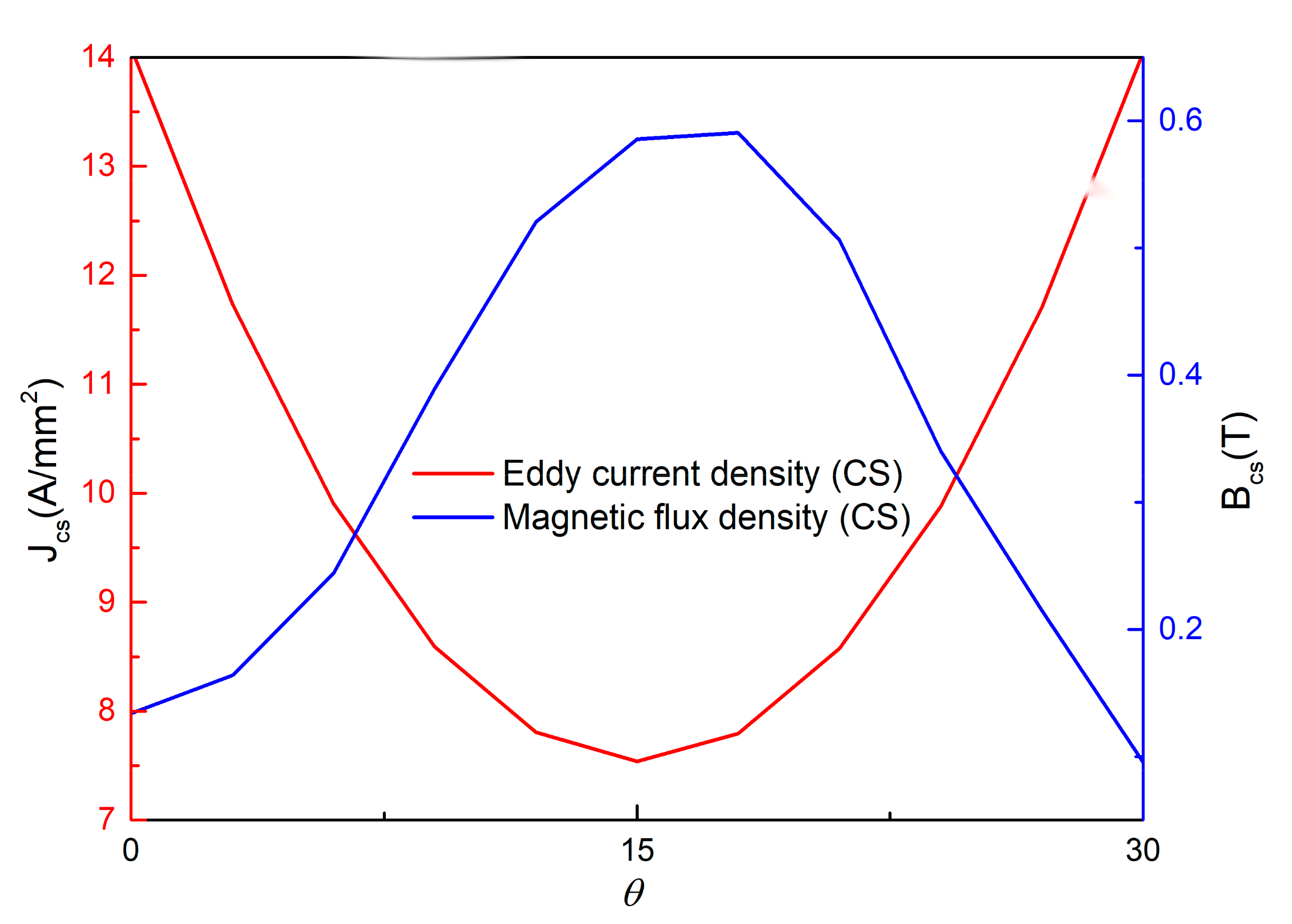
4.2. Analysis of Magnetic Field on the CS

The magnetic flux density and the eddy current are significant for the loss analysis of the APMC. As presented in Figure 8a, the magnetic flux density distributions on the surface of the CS seen from z-axis correspond to the alternating distributions of the PMs (N/S), in which the slip speed is set to 50 r/min. Obviously, the peak value of the magnetic density on the surface of the CS is 0.62T, while the location of the minimum value is between N-pole and S-pole of the PMs. Also, we can obtain the eddy current distributions on the surface of the CS again this FEM model, as shown in Figure 8b. Different from the magnetic flux density, the center of the eddy currents is situated between N-pole and S-pole of the PMs. Corresponding to the number of the PMs, the number of the eddy currents is 2p. In addition, the adjacent eddy currents are in opposite direction owing to the alternating magnetic poles.

Clearly, corresponding to the distributions in Figure 8 and Figure 9 depicts the relationship for the magnetic flux density (B_cs) and the eddy current density (J_cs) of the CS varying with different positions (θ) wherein θ₁ = 0° and θ₂ = 30° (360°/2p). Thanks to Faraday’s law of electromagnetic induction, the region with the strongest magnetic flux density is the weakest eddy current density.

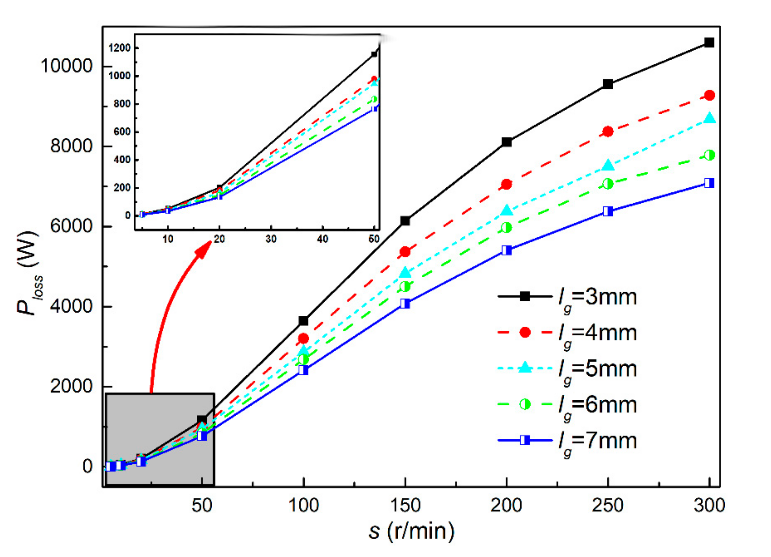
4.3. Loss Calculation

Accurately calculating the loss is essential to study the temperature rise for ensuring reliable operation. On account of skin effect, the eddy currents mainly concentrated on the surface of the CS. Therefore, we only consider the eddy current loss generated on the CS and ignore other losses, like mechanical loss. Based on the magnetic field analysis and Equation (2) belonging to an embedded algorithm in the FEM, the loss results under different air-gap lengths and slips are displayed in Figure 10. Obviously, with the increase of the slip speed (s), the loss increases continuously, while the loss decreases gradually with the increase of the air-gap length.

$$P_{cs}=1/{\sigma }_{cs}{\displaystyle {\int }_V\left|\mathbf{J}\right|}dV$$

(2)

where V is the volume of an integral region, and J is the vector of eddy current density.

$$\left\{\begin{array}{l}{P}_{loss}=k_c{P}_{cs}\\ k_c=1-\frac{\tanh (\pi w_{pm}/2{\tau }_p)}{(\pi w_{pm}/2{\tau }_p)[1+\tanh (\pi w_{pm}/2{\tau }_p)\tanh (\pi w_{cs}/{\tau }_p)]}\end{array}\right.$$

(3)

where w_pm = r_p2 − r_p1 and w_cs = (r₂ − r₁ − w_pm)/2.

However, the loss results in Figure 9 do not take into account 3-D edge effect. In view of this, Figure 11 shows the real eddy current paths on the CS where only the central region plays a role. In order to solve this problem, the correction factor (k_c), also called Russell–Norsworthy correction factor [6,11], is adopted as Equation (3).

5. LPTN Model

5.1. LPTN Model

The proposed LPTN model, including thermal nodes distribution and equivalent LPTN are exposed in Figure 12. Because of the rotational axisymmetry, only three PMs are presented in Figure 12a, where the view is obtained from the average radius of the PM (r = r_a). In this model, the thermal modes are located at different components involving ambient, iron yoke, CS, air-gap, PM holder, PM an iron yoke. Totally, there are 22 nodes (0~22) in this thermal network. In addition, the thermal nodes in Figure 12b are divided into red and black types, in which the power loss computed in the previous section are injected into the red nodes. It is worth noting that only conduction heat transfer and convection heat transfer are considered, not existing radiation heat transfer nearly.

In addition, providing that the APMC is divided into 2p parts, the nodes 2, 13, and 20 in Figure 12b are given different proportional losses respectively, as follows:

$$\left\{\begin{array}{c}{P}_{loss}^{13}=P_{loss}^{20}=\alpha P_{loss}/2p\\ P_{loss}^2=(1-\alpha )P_{loss}/2p\end{array}\right.$$

(4)

where α = τ_m/τ_p, representing the non-PM proportion after being divided into 2p parts.

5.2. Calculation for Thermal Resistances

• Conduction heat transfer: The region not in contact with air belongs to conduction heat transfer, as follows: inside the iron yoke (R_1~14, R_1~21, R_7~8 and R_7~15); inside the CS (R_2~13 and R_2~20); between the iron yoke and the CS (R_1~2, R_13~14 and R_20~21); inside the PM holder (R_4~11, R_4~18, R_9~10, R_10~11, R_16~17 and R_17~18); between the PM and the PM holder (R_4~5, R_5~10, R_5~17, R_6~9 and R_6~16); inside the PM (R_5~6); between the PM and the iron yoke (R_6~7); between the PM holder and the iron yoke (R_8~9 and R_15~16). Conduction thermal resistances can be obtained as [23,29]

  $$R=\frac{L}{kA}$$

  (5)

  where L (m) is the transfer path length, k (W/(m·°C) is the thermal conductivity of the material and A (m²) is the transfer path area. Here,

  Table 2. Thermal Conductivity of the Materials.

  Material	Symbol	Value (W/(m·°C))
  Steel	kst	36
  Copper	kcop	390
  Aluminum	kal	237
  Nd-Fe-B	knd	9
  Air	ka	0.026

  presents the thermal conductivity of the materials.

Using Equation (5), all the conduction thermal resistances can be found in Appendix A.

2.

Equivalent conduction/convection heat transfer: Since it is difficult to determine the flow condition in the air-gap, the air in the air gap can be regarded as a solid for convenience of calculation, that is, the convection heat transfer phenomenon in the air-gap can be simulated with a given air gap equivalent thermal conductivity. For the air-gap, corresponding to node 3, the equivalent heat transfer coefficient (h_air) can be calculated empirically as

$$\left\{\begin{array}{l}{v}_{air}=\pi (n_{in}-n_{out})(r_2+r_{p2})/60\\ {\mathrm{Re}}_{air}=v_{air}{l}_g/\gamma \\ h_{air}=0.0019{(l_g/r_2)}^{-2.9084}{\mathrm{Re}}_{air}{}^{0.4614\ln [3.33361(l_g/r_2)]}\end{array}\right.$$

(6)

where v_air is the airflow velocity in the air gap, Re_air is the Reynolds number for the air-gap and γ is the kinematic viscosity of air.

Then, employing Equations (5) and (6), R_2~3, R_3~4, R_3~12, R_3~19, R_11~12, R_12~13, R_18~19 and R_19~20 can be found in Appendix B.

3.

Convection heat transfer: In Figure 12, convection heat transfer certainly occurs between ambient node 0 and other nodes. Generally, as fluid flows, natural convection or forced convection would occur. The former is caused by the nonuniformity of the temperature or concentration; the latter relies on an external force, such as a pump or fan. For the studied APMC, although there is no pump or fan, the heat transfer belongs to forced convection because of the rotational motion of the CS and the PM holder. Convection thermal resistances can be obtained as [29]

$$R=\frac{1}{hA}$$

(7)

where h (W/(m·°C)) is the convection heat transfer coefficient, and A (m2) is the transfer path area.

In the ambient, corresponding to node 0, the convection heat transfer coefficient (h_am) can be calculated by

$$\left\{\begin{array}{l}{h}_{am}=13.3(1+v_{am}{}^{0.5})\\ v_{am}=\pi (n_{in}+n_{out})(r_2+r_{p2})/120\end{array}\right.$$

(8)

wherein v_am is the airflow velocity in the ambient.

Based on Equations (6) to (8), the convection thermal resistances can be found in Appendix C.

5.3. Calculation for Temperature Rise

For the LPTN model, the temperature rise of each node can be solved by

$$[G][T]=[P]$$

(9)

where [P] is the column matrix of nodal power loss, [G] is the thermal conductance matrix and [T] is the temperature rise vector. The thermal conductance matrix can be defined by

$$[G]=\left[\begin{array}{cccc}{\displaystyle \sum _{i=1}^n\frac{1}{R_{1\text{~}i}}}& -\frac{1}{R_{1~2}}& \cdots & -\frac{1}{R_{1~n}}\\ -\frac{1}{R_{2~1}}& {\displaystyle \sum _{i=1}^n\frac{1}{R_{2~i}}}& \cdots & -\frac{1}{R_{2~n}}\\ ⋮& ⋮& \ddots & ⋮\\ -\frac{1}{R_{n~1}}& -\frac{1}{R_{n~2}}& \cdots & {\displaystyle \sum _{i=1}^n\frac{1}{R_{n~i}}}\end{array}\right]$$

(10)

where n is the number of all the nodes for the LPTN model, and R_i~j represents the thermal resistance between adjacent nodes i and node j. Besides, 1/R_i~j is normally ignored because there is no heat exchange between itself and R_i~j = R_j~i.

Accounting for the effect of ambient temperature, Equation (9) is not perfect to solve the temperature rise of the APMC. Thus, a modified equation for Equation (9) is offered as

$$[T]=\{[P]-T_0[G_0]\}{[G]}^{-1}$$

(11)

where T₀ is the local ambient temperature in accordance with the room temperature of the experiment, and [G₀] = [−1/R_1~0, −1/R_2~0, …, −1/R_n~0].

Besides, the node temperature in the same region is averaged as the calculation result. For example, the average value of nodes 2, 13 and 20 is taken as the temperature result of the CS.

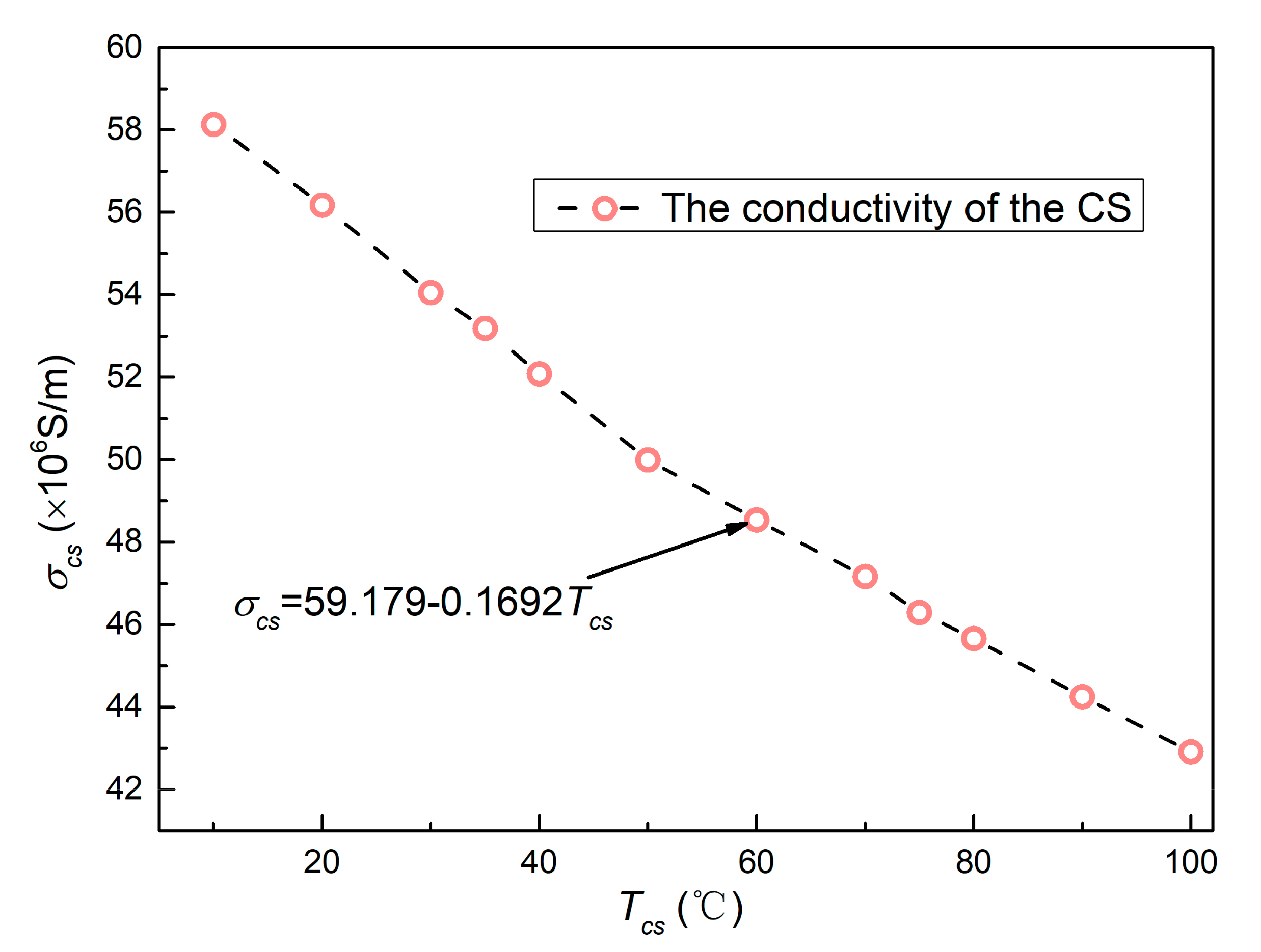
5.4. Adjusting the Conductivity of the CS

Additionally, the column matrix of nodal power loss is temperature-dependent and require temperature update in the thermal analysis strategy. As a result, an iterative coupled electromagnetic and thermal modeling, corresponding to Figure 4, must be employed in this section. Here, the conductivity of the CS is the most crucial factor for updating the nodal power loss and temperature. Figure 13 gives the relationship between the conductivity of the CS (σ_cs) and different temperature (T_cs), which provides an effective reference for adjusting the conductivity of the CS. This iteration process is generally over until a set convergence threshold (T_s) is met, such as 1%.

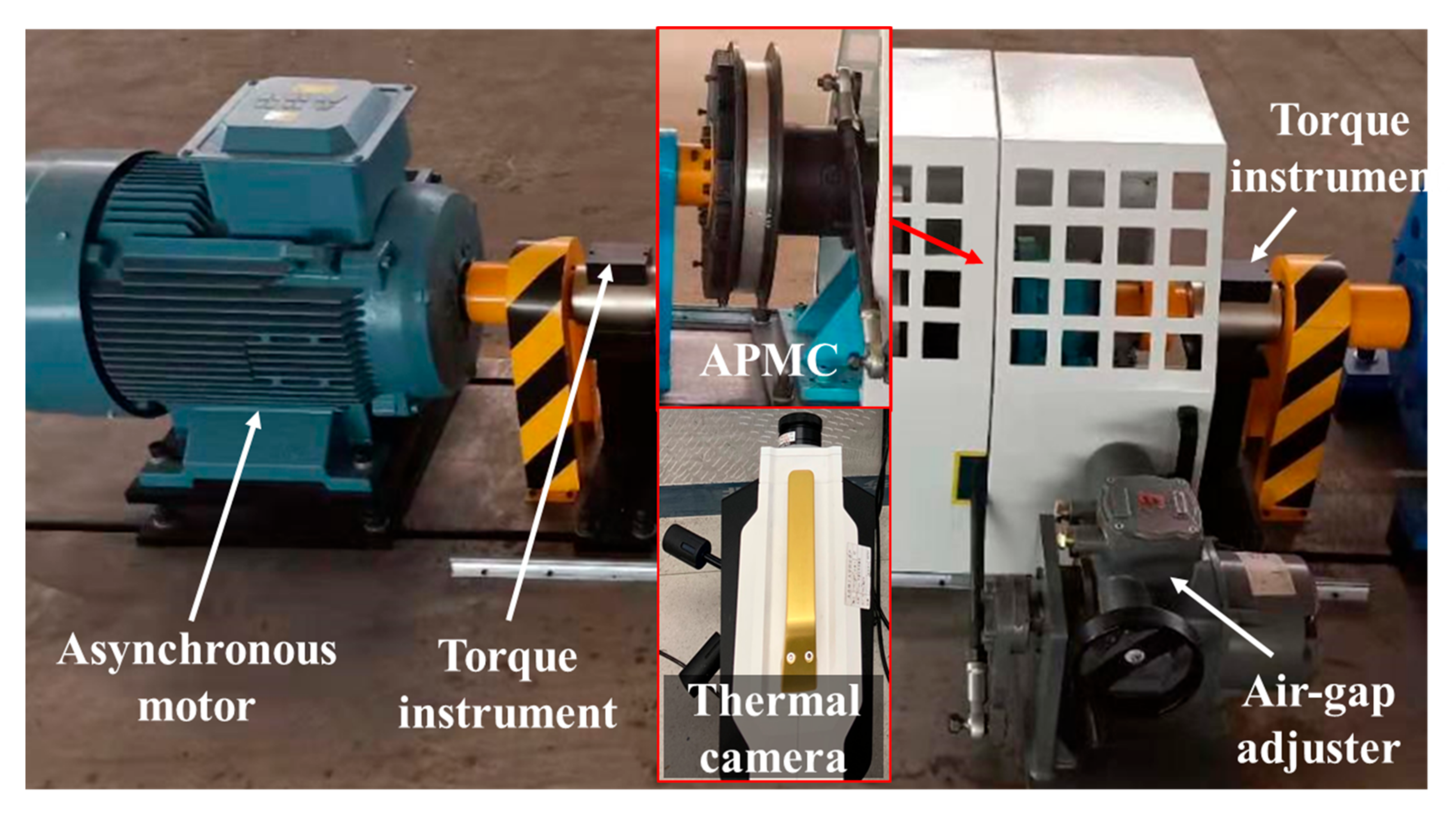
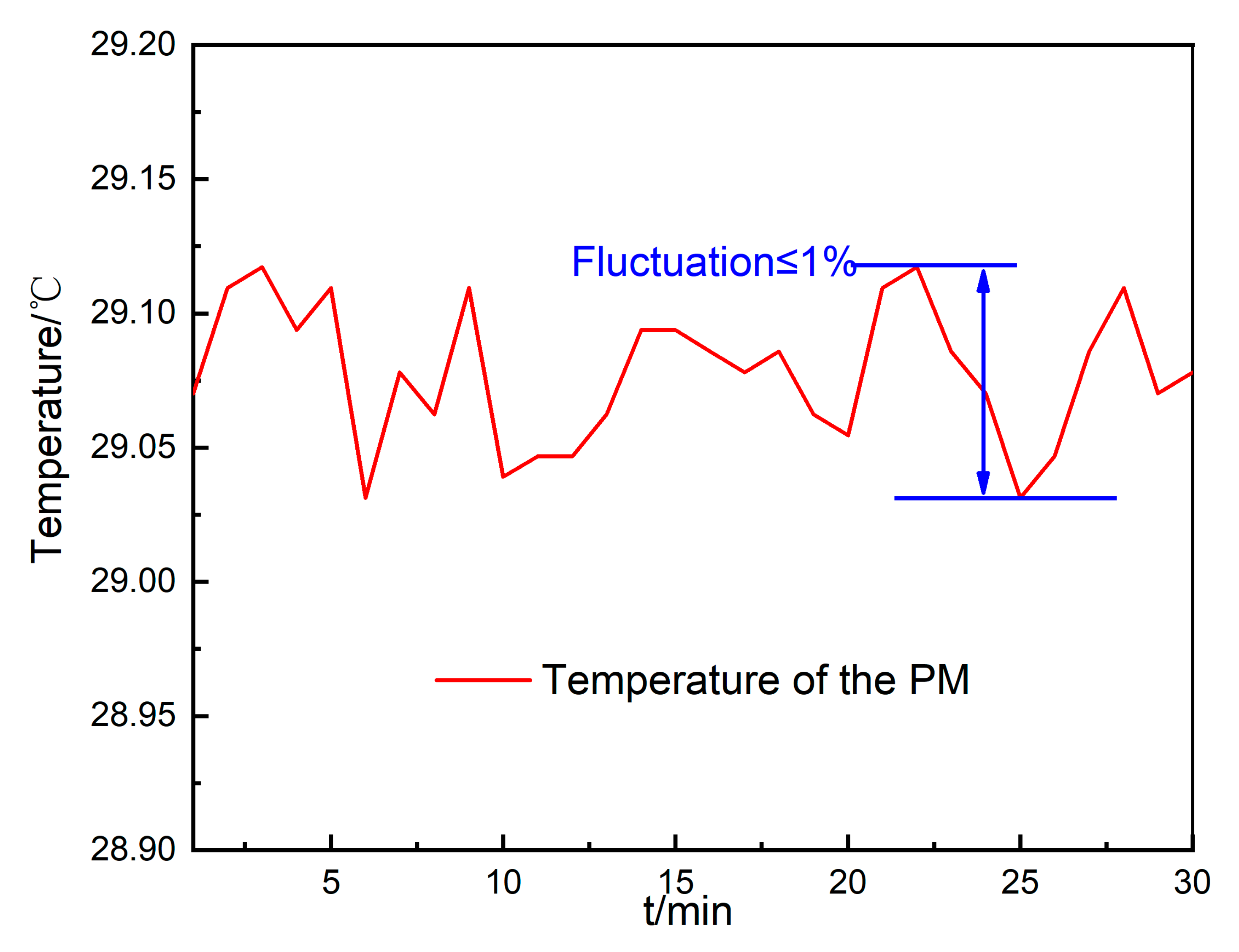
6. Experiment Verification

In order to verify the thermal analysis strategy proposed in this paper, the experiment platform for the studied APMC is built in Figure 14. Since the APMC is in the state of high-speed rotation, the traditional static temperature measurement method cannot be carried out. Thus, a high-precision thermal camera, labeled as Telops FAST V100k, (Telops Inc, Montreal, Quebec, Canada.) is used to measure the temperature. The thermal camera was set up half a meter away from the APMC. After the APMC was in stable operation, the PM module and CS module were photographed. Since the interior of the components could not be photographed, surface temperature data was used as experimental results. However, the experimental results are generally obtained when the APMC operates for one hour to reach the thermal balance. Also, the cross-section of the LPTN model inside the components is about 10 mm away from the surface. Therefore, it is considered that the error between the internal temperature of this cross-section and surface temperature is not large.

Besides, if the uniformity of measured temperature is well, and the fluctuation is less than 1%, the measured results can be used, as shown in Figure 15. Also, Figure 16 presents a measurement result by thermal camera in the case of ‘l_g = 5 mm and s = 20 r/min’. The measured results can be obtained by taking the points. Specifically, in the post-processing of the thermal camera software, some points in the photographed area are selected as the temperature results of each component.

Here, the temperature of the CS and the PM is of greatest concern. As shown in Figure 17, compared with the experiment results at different slip speed, the proposed thermal analysis strategy for APMCs are in good agreement, and the relative error is within 6.7%. Moreover, the demagnetization temperature of the PM used in this paper is 180 ℃. Therefore, the slip speed of 120r/min is the limit from Figure 17. If selected PM has a higher demagnetization temperature, a greater slip speed can be achieved.

In order to further verify the accuracy of the strategy, Figure 18 presents the comparison between the proposed strategy and experiment under different air-gaps and slip speeds. With the increase of l_g, the temperature of PM decreases gradually. As can be seen from Figure 18, the strategy has a good coincidence with the experimental results, with the error less than 6.7%.

In the practical design and optimization of APMCs, the pole-pairs number of the PMs and the thickness of the CS are two important parameters. Besides, the temperature of the PM is key for the safe operation of APMCs due to demagnetization effect. Through the proposed strategy, Figure 19 presents the relationship between the temperature of the PM and the pole-pairs number of the PMs (p) at s = 120 r/min. From Figure 19, with the increase of p, the temperature of the PM increases gradually. Taking the demagnetization effect into account, selecting p as 6 is appropriate. Moreover, by the proposed strategy, Figure 20 presents the relationship between the temperature of the PM and the thickness of the CS (l_cs) at s = 120 r/min. From Figure 20, with the increase of l_cs, the temperature of the PM decreases gradually. Taking the demagnetization effect into account, selecting l_cs ≥6 is appropriate. However, in order to avoid excessive mass, selecting l_cs as 6 is optimal.

7. Conclusions

A thermal analysis strategy is proposed to obtain the temperature results for APMCs, which combines FEM with LPTN. Firstly, the manufactured prototype of the studied APMC is built as well as giving its parameters. This proposed strategy is an iterative process considering some assumptions. Secondly, the magnetic field employing the FEM is offered to obtain the loss generated on the CS, where the magnetic field of the CS is analyzed. Then, the source nodes are assigned losses to calculate the matrix of the LPTN model and get the temperature results by adjusting the conductivity of the CS. Finally, the strategy is verified by experiment results where its relative error is less than 6.7%. In summary, the strategy developed in this paper can provide constructive references for operation safety of APMCs.

References

1. Ye, L.Z.; Li, D.S.; Ma, Y.J.; Jiao, B.F. Design and Performance of a Water-cooled Permanent Magnet Retarder for Heavy Vehicles. IEEE Trans. Energy Convers. 2011, 26, 953–958. [Google Scholar] [CrossRef]
2. Li, Y.B.; Lin, H.Y.; Huang, H.; Yang, H.; Tao, Q.C.; Fang, S.H. Analytical Analysis of a Novel Brushless Hybrid Excited Adjustable Speed Eddy Current Coupling. Energies 2019, 12, 308. [Google Scholar] [CrossRef] [Green Version]
3. Mohammadi, S.; Mirsalim, M.; Vaez-Zadeh, S.; Talebi, H.A. Analytical Modeling and Analysis of Axial-Flux Interior Permanent-Magnet Couplers. IEEE Trans. Ind. Electron. 2014, 61, 5940–5947. [Google Scholar] [CrossRef]
4. Lubin, T.; Mezani, S.; Rezzoug, A. Simple Analytical Expressions for the Force and Torque of Axial Magnetic Couplings. IEEE Trans. Energy Convers. 2012, 27, 536–546. [Google Scholar] [CrossRef] [Green Version]
5. Wang, S.; Guo, Y.C.; Cheng, G.; Li, D.Y. Performance Study of Hybrid Magnetic Coupler Based on Magneto Thermal Coupled Analysis. Energies 2017, 10, 1148. [Google Scholar] [CrossRef] [Green Version]
6. Wang, J.; Zhu, J.G. A Simple Method for Performance Prediction of Permanent Magnet Eddy Current Couplings Using a New Magnetic Equivalent Circuit Model. IEEE Trans. Ind. Electron. 2018, 65, 2487–2495. [Google Scholar] [CrossRef]
7. Dai, X.; Liang, Q.H.; Cao, J.Y.; Long, Y.J.; Mo, J.Q.; Wang, S.G. Analytical Modeling of Axial-Flux Permanent Magnet Eddy Current Couplings With a Slotted Conductor Topology. IEEE Trans. Magn. 2016, 52, 15. [Google Scholar] [CrossRef]
8. Lubin, T.; Mezani, S.; Rezzoug, A. Experimental and Theoretical Analyses of Axial Magnetic Coupling Under Steady-State and Transient Operations. IEEE Trans. Ind. Electron. 2014, 61, 4356–4365. [Google Scholar] [CrossRef] [Green Version]
9. Mohammadi, S.; Mirsalim, M. Double-sided permanent-magnet radial-flux eddy-current couplers: Three-dimensional analytical modelling, static and transient study, and sensitivity analysis. IET Electr. Power Appl. 2013, 7, 665–679. [Google Scholar] [CrossRef]
10. Ravaud, R.; Lemarquand, V.; Lemarquand, G. Analytical Design of Permanent Magnet Radial Couplings. IEEE Trans. Magn. 2010, 46, 3860–3865. [Google Scholar] [CrossRef]
11. Mohammadi, S.; Mirsalim, M.; Vaez-Zadeh, S. Nonlinear Modeling of Eddy-Current Couplers. IEEE Trans. Energy Convers. 2014, 29, 224–231. [Google Scholar] [CrossRef]
12. Fei, W.Z.; Luk, P.C.K. Torque Ripple Reduction of a Direct-Drive Permanent-Magnet Synchronous Machine by Material-Efficient Axial Pole Pairing. IEEE Trans. Ind. Electron. 2012, 59, 2601–2611. [Google Scholar] [CrossRef] [Green Version]
13. Min, K.C.; Choi, J.Y.; Kim, J.M.; Cho, H.W.; Jang, S.M. Eddy-Current Loss Analysis of Noncontact Magnetic Device with Permanent Magnets Based on Analytical Field Calculations. IEEE Trans. Magn. 2015, 51, 4. [Google Scholar] [CrossRef]
14. Choi, J.Y.; Jang, S.M. Analytical magnetic torque calculations and experimental testing of radial flux permanent magnet-type eddy current brakes. J. Appl. Phys. 2012, 111, 3. [Google Scholar] [CrossRef]
15. Dai, X.; Cao, J.Y.; Long, Y.J.; Liang, Q.H.; Mo, J.Q.; Wang, S.G. Analytical Modeling of an Eddy-current Adjustable-speed Coupling System with a Three-segment Halbach Magnet Array. Electr. Power Compon. Syst. 2015, 43, 1891–1901. [Google Scholar] [CrossRef]
16. Wang, J.; Lin, H.Y.; Fang, S.H.; Huang, Y.K. A General Analytical Model of Permanent Magnet Eddy Current Couplings. IEEE Trans. Magn. 2014, 50, 9. [Google Scholar] [CrossRef]
17. Lubin, T.; Rezzoug, A. Steady-State and Transient Performance of Axial-Field Eddy-Current Coupling. IEEE Trans. Ind. Electron. 2015, 62, 2287–2296. [Google Scholar] [CrossRef] [Green Version]
18. Dolisy, B.; Mezani, S.; Lubin, T.; Leveque, J. A New Analytical Torque Formula for Axial Field Permanent Magnets Coupling. IEEE Trans. Energy Convers. 2015, 30, 892–899. [Google Scholar] [CrossRef] [Green Version]
19. Lubin, T.; Rezzoug, A. 3-D Analytical Model for Axial-Flux Eddy-Current Couplings and Brakes Under Steady-State Conditions. IEEE Trans. Magn. 2015, 51, 12. [Google Scholar] [CrossRef] [Green Version]
20. Wang, J.; Lin, H.Y.; Fang, S.H. Analytical Prediction of Torque Characteristics of Eddy Current Couplings Having a Quasi-Halbach Magnet Structure. IEEE Trans. Magn. 2016, 52, 9. [Google Scholar] [CrossRef]
21. Li, Z.; Wang, D.Z.; Zheng, D.; Yu, L.X. Analytical modeling and analysis of magnetic field and torque for novel axial flux eddy current couplers with PM excitation. AIP Adv. 2017, 7, 13. [Google Scholar] [CrossRef] [Green Version]
22. Lubin, T.; Rezzoug, A. Improved 3-D Analytical Model for Axial-Flux Eddy-Current Couplings with Curvature Effects. IEEE Trans. Magn. 2017, 53, 9. [Google Scholar] [CrossRef]
23. Huang, X.Z.; Li, L.Y.; Zhou, B.; Zhang, C.M.; Zhang, Z.R. Temperature Calculation for Tubular Linear Motor by the Combination of Thermal Circuit and Temperature Field Method Considering the Linear Motion of Air Gap. IEEE Trans. Ind. Electron. 2014, 61, 3923–3931. [Google Scholar] [CrossRef]
24. Lu, Y.P.; Liu, L.; Zhang, D.X. Simulation and Analysis of Thermal Fields of Rotor Multislots for Nonsalient-Pole Motor. IEEE Trans. Ind. Electron. 2015, 62, 7678–7686. [Google Scholar] [CrossRef]
25. Vese, I.C.; Marignetti, F.; Radulescu, M.M. Multiphysics Approach to Numerical Modeling of a Permanent-Magnet Tubular Linear Motor. IEEE Trans. Ind. Electron. 2010, 57, 320–326. [Google Scholar] [CrossRef]
26. Zhu, X.Y.; Wu, W.Y.; Yang, S.; Xiang, Z.X.; Quan, L. Comparative Design and Analysis of New Type of Flux-Intensifying Interior Permanent Magnet Motors with Different Q-Axis Rotor Flux Barriers. IEEE Trans. Energy Convers. 2018, 33, 2260–2269. [Google Scholar] [CrossRef]
27. Le Besnerais, J.; Fasquelle, A.; Hecquet, M.; Pelle, J.; Lanfranchi, V.; Harmand, S.; Brochet, P.; Randria, A. Multiphysics Modeling: Electro-Vibro-Acoustics and Heat Transfer of PWM-Fed Induction Machines. IEEE Trans. Ind. Electron. 2010, 57, 1279–1287. [Google Scholar] [CrossRef]
28. Sun, X.K.; Cheng, M. Thermal Analysis and Cooling System Design of Dual Mechanical Port Machine for Wind Power Application. IEEE Trans. Ind. Electron. 2013, 60, 1724–1733. [Google Scholar] [CrossRef]
29. Mo, L.H.; Zhang, T.; Lu, Q. Thermal Analysis of a Flux-Switching Permanent-Magnet Double-Rotor Machine with a 3-D Thermal Network Model. IEEE Trans. Appl. Supercond. 2019, 29, 5. [Google Scholar] [CrossRef]
30. Valenzuela, M.A.; Ramirez, G. Thermal Models for Online Detection of Pulp Obstructing the Cooling System of TEFC Induction Motors in Pulp Area. IEEE Trans. Ind. Appl. 2011, 47, 719–729. [Google Scholar] [CrossRef]
Figure 1. Configuration of an axial permanent magnet coupling.
Energies 13 05019 g001
Figure 2. The geometry of the studied APMC (p = 6) with its exploded view and geometrical parameters.
Energies 13 05019 g002
Figure 3. The manufactured prototype of the studied APMC (lg = 30 mm).
Energies 13 05019 g003
Figure 4. The procedure of the thermal analysis strategy.
Energies 13 05019 g004
Figure 5. Nonlinear B–H curve (1010 steel) for the iron yokes.
Energies 13 05019 g005
Figure 6. The mesh size for all the components used in the FEM.
Energies 13 05019 g006
Figure 7. Mesh in 3D of the FEM model.
Energies 13 05019 g007
Figure 8. Magnetic field analysis (z-axis, p = 6 and s = 50 r/min): (a) the magnetic flux density distributions, (b) the eddy current distributions.
Energies 13 05019 g008
Figure 9. The curves for depicting the distributions on the CS.
Energies 13 05019 g009
Figure 10. The loss results under different air-gap lengths and slips using FEM.
Energies 13 05019 g010
Figure 11. The real eddy current paths on the CS.
Energies 13 05019 g011
Figure 12. Proposed LPTN model: (a) thermal nodes distribution, (b) equivalent LPTN.
Energies 13 05019 g012
Figure 13. The relationship between the conductivity of the CS and different temperature.
Energies 13 05019 g013
Figure 14. The experiment platform for the studied APMC.
Energies 13 05019 g014
Figure 15. Temperature variation of the PM within 30 min (s = 25 r/min).
Energies 13 05019 g015
Figure 16. Temperature measurement results obtained by thermal camera (lg = 5 mm and s = 20 r/min).
Energies 13 05019 g016
Figure 17. Comparison between the proposed strategy and experiment (lg = 5 mm).
Energies 13 05019 g017
Figure 18. Comparison between proposed strategy and experiment under different air-gaps and slip speeds.
Energies 13 05019 g018
Figure 19. The relationship between the temperature of the PM and the pole-pairs number of the PMs. (s = 120 r/min).
Energies 13 05019 g019
Figure 20. The relationship between the temperature of the PM and the thickness of the CS (s = 120 r/min).
Energies 13 05019 g020